Purchasing Power Parity (PPP)
Deviations: The case of H&M.
BACHELOR THESIS WITHIN: Economics CREDITS: 15
PROGRAMME: International Economics
AUTHORS: Sofia Chen Ruoshui He JÖNKÖPING May 2020
i
Bachelor Degree Project in Economics
Title:
Purchasing Power Parity (PPP) Deviations: The case of H&M.
Authors:
Sofia Chen and Ruoshui He
Tutor:
Andrea Schneider
Date:
2020-05-18
Key terms: Purchasing power parity, law of one price, homogenous products, price settings,
H&M.
Abstract
The theories of the law of one price and purchasing power parity are thought to hold almost
exactly in financial market, but it seems less likely to occur in international trade where arbitrage
opportunities take place. The purpose of this study is to test whether the purchasing power parity
holds for commodities in various national markets, for which a quantitative method is followed.
For identical goods, the prices should be equal across countries. In fact, the prices vary
significantly across ‘truly homogenous’ goods within a product group. The finding suggests that
differences in productivity and value-added tax do have significant positive impacts on price
settings. As a consequence, purchasing power parity definitely does not prevail as well as law of
one price does not. Further studies can use these findings to examine the extent and permanence
of violations of the law of one price.
ii
Table of Contents
1 Introduction ... 1
2 Theoretical Framework ... 3
2.1
The Law of One Price ... 3
2.2
Purchasing Power Parity ... 3
2.2.1 Absoulte PPP ... 4
2.2.2 Relative PPP ... 6
2.3
Purchasing Power Parity Deviation Puzzle ... 7
2.3.1 Trade Barriers ... 7
2.3.2 Non-tradable Inputs ... 8
2.3.3 Value-added Tax ... 9
3 Literature Review ... 11
4 Empirical Analysis ... 12
4.1
Data ... 12
4.2
Empirical Models ... 19
4.3
Empirical Findings ... 21
4.4
Limitations ... 26
5 Conclusion ... 27
References ... 28
Appendix ... 33
iii
Figures
Figure 1 The Effect of Tariff in Export and Import Countries...7
Figure 2 The Tariff Rate of Ten Countries...8
Figure 3 Product Image...12
Figure 4 The VAT Rate Distribution in Ten Countries...16
Figure 5 The Silk Shirt Dress Price Distribution...17
Figure 6 Comparison of The H&M Index (Silk Shirt Dress) with The Big Mac Index...17
Figure 7 Comparison of The H&M Index (Patterned Jeans) with The Big Mac Index...19
Figure 8 Ten Countries Productivity...20
Tables
Table 1 The Big Mac Index...5
Table 2 Product Description...12
Table 3 The Products Prices List in Ten Countries...13
Table 4 Exchange Rate...14
Table 5 The Products Prices List in Common Currency...15
Table 6 The Products Prices List in Common Currency without VAT...16
Table 7 The Regression Output for Model One...22
1
1 Introduction
With the rapid growth of electronic commerce in the globalized world, online shopping has become one of the most convenient ways to make comparisons of similar products in different markets. This can be credited to consumers who are always able to convert prices into another currency by which to determine whether it is profitable to purchase goods in the particular market. Currently, H&M is one of the most visited fashion sites in the world1. As a consumer, if
we solely look at the price of one identical good for say, Jersey T-shirt sold by H&M in Sweden and China. In fact, the product sold more expensive in China than in Sweden when measured in a common currency. This phenomenon, however, is related to the theory of purchasing power parity.
Purchasing power parity (PPP) is one of the oldest and most fundamental economics concepts (Krugman, Obstfeld, & Melitz, 2012). It states that the price levels between any two countries should be identical after converting them into a common currency. As a theoretical proposition, it is widely used in the economic literature to analyze and to predict exchange rate movements as well as to serve as conditions under which international markets adjust to attain long-term equilibrium. The law of one price (LOP) does not focus on the aggregate price level. It points out that the price of each identical good is the same in different markets when expressed in a common currency. If the law of one price leads to the equalization of a commodity price between two markets, then it seems reasonable to conclude that purchasing power parity that describes the equality of market baskets of goods across countries should also hold.
Ideally, the test of LOP and PPP is to compare the prices of two transactions, where the buyer is the only difference in the characteristics of the transaction. In practice, the assumption of homogenous goods is almost violated in available data or on complex products to some extent. The study of Goldberg and Verboven (1998) uses a complex product, car, to examine PPP deviations. The selected product, however, is usually not exactly identical in different countries. Subsequent research attempted to focus on homogeneous products of specific companies that are sold in various national markets. The most well-known study is the Big Mac Index published by The Economist in 19862, which was treated as an example of "truly homogenous"
products since the Big Macs with the same taste, ingredients, and appearance sold by McDonald’s everywhere. This paper continues to use price information on various identical products sold by a single firm that provides standardized services in various national markets in a standardized environment in undertaking this research.
This paper chose the clothing industry to investigate the nature of price differences. This is due to the fact that it plays a decisive role in past economic development. Palpacuer, Gibbon and Thomsen (2004) claim that the clothing industry has played several vital roles in the development process. It reduced unemployment by targeting unskilled labor, satisfied the needs of a large number of people through mass production as well as created capital for more technical demanding production in other sectors. A large number of clothing exports provided funding for the import of more advanced technologies. Furthermore, it is significantly important for employment and growth in developing countries. Hence, one of the well-established firms in the clothing industry - H&M has been selected.
1 H&M Group
-https://hmgroup.com/content/dam/hmgroup/groupsite/documents/masterlanguage/Annual%20R eport/HM_Annual%20Report%202019.pdf
2
H&M is founded in 1947 in Västerås, Sweden. During the past 70 years, it gradually developed into one of the most famous worldwide clothing companies. Nowadays, H&M operates in 74 countries with over 5,000 stores under various company brands3. Their products are classified
into several departments, including categories of clothes, cosmetics, home decorations, and textiles. This provides basic popularity for all consumers in terms of men, women as well as kids. H&M sold homogenous products in an identical shopping environment with standardized services in various national markets considered to be one of the interesting cases in testing the PPP deviations. Moreover, the above illustrative example is contrary to the theory of PPP. It is of great interest and motivation to study if the situation is held for other H&M products in a large sample of various national markets.
This paper is designed to investigate the purchasing power parity deviations using the case of H&M. The aim of this paper is to analyze whether product prices are the same across countries when the prices are measured in a common currency. If the common-currency prices of identical H&M products are not the same in different markets, the PPP is thus not held and the PPP deviations exist. Further research is necessary to identify which variables contribute to the price discrepancies. The five products, Silk Shirt Dress, Nylon Windbreaker, Platform Satin Boots, Patterned Jeans, and Cotton Pile Rug are selected based on different H&M categories. The main focus relies on the price levels of the five identical products in ten countries incorporating three different regions: North America, Asia Pacific, and Europe. This paper aims to answer the research question of whether purchasing power parity holds for H&M whilst to figure out the contributions to price discrepancies if PPP does not prevail. Moreover, our analysis allows us to discuss which currencies are undervalued or overvalued examined by the H&M Index. A further comparison is necessary to see if they are the same as if we use the Big Mac Index.
This paper is organized as the following outlines: Section 2 outlays the relevant theories of LOP and PPP whilst interprets its implications briefly. Section 3 reviews various previous research that carry out empirical studies of the LOP and PPP. Section 4 describes the data and empirical models as well as develops the hypotheses to be tested. The empirical results will be analyzed based on the regression outputs and the results will be compared to results from a previous academic literature afterwards. Section 5 concludes the overall findings and suggests further studies.
3 H&M Group -
https://hmgroup.com/content/dam/hmgroup/groupsite/documents/masterlanguage/Annual%20R eport/HM_Annual%20Report%202019.pdf
3
2 Theoretical Framework
In this chapter, the theories of law of one price and purchasing power parity will be reviewed and its fundamental implication will be discussed. Additionally, several possible reasons for PPP deviations are illustrated in the purchasing power parity deviation puzzle.
2.1 The Law of One Price
Milton Friedman (1953) proposed the economic theory of law of one price (LOP). It states that in a perfect frictionless market, the price of homogeneous goods will be the same in different locations after taking the exchange rate into consideration. The real value of any identical commodity is consistently held across countries due to arbitrage opportunities. If the prices of the same commodity differ from each other in the entire market, the arbitrage opportunity arises since a trader can buy a commodity at a lower price and then immediately sell the commodity in another market at a higher price to obtain a net profit. Economic theory states that subsequently, the forces of supply and demand will converge the prices of the entire market closer to each other. Increase in demand for one good push up price in the low-priced market while the increase in the supply of that good force price down in the high-priced market. As a consequence, arbitrage opportunities will be eliminated and thus LOP primarily holds.
𝑃 = 𝐸 × 𝑃∗ (1)
Equation (1) says the price (P) of any good in domestic currency should be equal to the price ( 𝑃∗ ) in consequence of the foreign currency multiplying the exchange rate (E). Equation (1) is
called the law of one price and it indicates that goods is sold for the same price worldwide. For instance, the recent exchange rate shows that 1 Swedish Krona (SEK) equals 0.1045 US dollars (USD), and a thick sweater is sold 100 SEK in Sweden and 10.45 in the U.S., then P= EP*= 0.1045*100 = 10.45. Thus, according to the LOP, the price of a thick sweater in Sweden is the same as the price in the U.S. once we convert the krona price into dollars using the exchange rate between dollar and krona. If prices are not the same across two countries, the arbitrage opportunity exists. It starts promoting the movement of goods between two markets, and this activity continuously proceeds until the prices are exactly the same.
The law of one price is based on several assumptions and prerequisites including the absence of trade frictions, free competition in the market, and price flexibility. Specifically, the LOP theory can only be achieved on a certain basis: 1) Complete information in all markets. 2) Zero tariffs. 3) Zero transaction cost. 4) The countries which are used for comparison have implemented the same criteria of free currency conversion, with entirely free circulation in the aspect of currency, goods, services, and capital.
2.2 Purchasing Power Parity
The law of one price is the foundation of purchasing power parity (PPP). ‘The notion of purchasing power parity has a long intellectual history and can be traced to the 16th-century writings of scholars from the University of Salamanca in Spain’ (Reinert, Rajan, Glass, & Davis, 2009, p. 942). The modern definition of PPP is usually credited to Gustav Cassel (1918). It portrays that in the absence of transaction costs and official barriers to trade, when a basket of the same goods is treated at the same price in two countries, the two currencies are of equal value. It ensures that buyers have the same purchasing power of the currency in global markets. PPP exchange rates are widely used to compare the standards of living across countries. It measures the price ratio of two or more currencies when buying the same quantity and quality
4
of certain goods and services in different locations. Absolute PPP and relative PPP are two statements of PPP based on the law of one price.
An amusing way of attempting to measure the PPP between different currencies and the US dollar is the Big Mac Index introduced by The Economist, which is a useful tool to predict exchange rate movement and to reflect the standard of living. Cumby (1996) states that the Big Mac parity seems to be helpful in forecasting relative local currency prices. When a country has a high US dollar price of Big Macs, the relative local currency price of Big Macs in that country is likely to fall during the following year. Dunn (2007) claims that the Big Mac is an almost ideal item to see if currencies are at or close to purchasing power parity because it is the same product in all countries and it is almost a pure nontradable. Atal (2014) finds out the per capita real income can be very low in some countries when Big Mac burgers are sold at very cheap prices in those countries.
A selection of Big Mac Index figures is shown in Table 1, which was published in The Economist in January 2020. The price of a Big Mac in the United States sold at 5.67 dollars and in the UK cost 3.39 pounds, the implied purchasing power parity equals £0.60 to $1. The actual exchange rate of the US dollar to the UK pound was 0.77 in January 2020. This indicates that the UK pound was undervalued against the US dollar by 22.08%. The undervaluation of the currency indicates that the cost of living in the UK is lower than in the U.S. In other words, by comparing the price of a Big Mac in various countries where McDonald’s operates, we are able to discover which currencies are undervalued and which are overvalued by which to measure the cost of living. However, some empirical studies examine the Big Mac Index as an exchange rate prediction tool that is only accurate on a certain basis. Portes and Atal (2014) find that there is some forecasting power in the Big Mac Index as countries gravitate towards a PPP rate for a particular group of high-income countries, but for a large group of emerging markets, their currencies’ path diverged from parity.
Undervaluation of a currency beneficial exports as price becomes relatively cheap in that country. Consumers tend to purchase more goods contributing to an increase in demand for the local currency on the foreign exchange market. On the other hand, consumers refrain from buying the more expensive foreign goods, reducing the supply of local currency in change for foreign currency. As a consequence, the local currency appreciates until reaching its PPP exchange rate. The foreign currency, by contrast, depreciates until it meets the PPP rate.
‘Purchasing power parity suggests that when the rate enables people in different countries to buy the same basket of goods with an equal amount of money, the exchange rate will be in long-run equilibrium. Therefore, in the long long-run, exchange rates should move towards levels that would equalize the prices of an identical basket of goods and services bought in either of the two countries whose exchange rate is being compared’ (Blink & Dorton, 2012, p. 286).
2.2.1 Absolute PPP
Absolute PPP indicates that the exchange rate between two currencies will be the ratio of aggregate price level in the two countries, meaning that the cost of any good in the same bundles should have equal value across countries after converting them into a common currency. The value of a country's currency and its demand are determined by the amount of goods and services that a unit currency can buy in the country, which refer to its purchasing power. The magnitude of purchasing power is reflected in the price level. According to this relationship, the rise in domestic prices shows the depreciation of the domestic currency relative to foreign currency. It is written in the second formula.
5
Table 1. The Big Mac Index4
Country In local Currency In US dollars Big Mac exchange rate (PPP) Actual dollar exchange rate Under (-) / Over (+) valuation against the
dollar, % United State $5.67 5.67 United Kingdom £3.39 5.67 0.60 0.77 -22.08 Canada C$6.77 5.67 1.19 1.31 -9.16 France €4.12 5.67 0.73 0.90 -18.89 Sweden SKr 51.50 5.67 9.08 9.46 -4.02 Switzerland SFr 6.50 5.67 1.15 0.97 18.56 Norway Nkr 53.00 5.67 9.35 8.88 5.29 China Yuan 21.50 5.67 3.79 6.88 -44.91 Japan Yen 390.00 5.67 68.78 110.04 -37.50
South Korea Won 4500.00 5.67 793.65 1156.10 -31.35
Israel Shekels 17.00 5.67 3.00 3.46 -13.29 Brazil Reais 19.90 5.67 3.51 4.14 -15.22 Singapore S$5.90 5.67 1.04 1.35 -22.96 New Zealand NZ$6.50 5.67 1.15 1.51 -23.84 Colombia Pesos 11900.00 5.67 2098.77 3287.63 -36.16 Chile Pesos 2640.00 5.67 465.61 772.74 -39.75 India Rupees 188.00 5.67 33.16 70.88 -53.22 Hong Kong HK$20.50 5.67 3.62 7.78 -53.47 Poland Zloty 11.00 5.67 1.94 3.80 -48.95 Pakistan Rupes 520.00 5.67 91.71 154.88 -40.79 Australia A$6.45 5.67 1.14 1.45 -21.38
6
Equation (2) is the general form of absolute PPP in which e represents the exchange rate of domestic currency to foreign currency, while P and 𝑃∗ represent the price of domestics and
foreign goods respectively. The preconditions of absolute PPP include: (1) the law of one price holds for any tradable commodity;
(2) in the compilation of the price index of the two countries, various tradable commodities should share equal weights.
Under the absolute PPP, the exchange rate between Australia and the U.S. equals the price level of the same market basket of goods in Australia divided by the price level of the same market basket of goods in the U.S. For example, based on the Big Mac Index in Table 1, the price level ratio of PAus/ PUS represents a PPP exchange rate of 1.14 AUD per 1 USD whereas the actual exchange rate (EAus/US) equals 1.45 AUD per 1 USD. According to the absolute PPP, the Australian dollar will appreciate against the US dollar by 21.38% or the US dollar will, in turn, depreciate against the Australian dollar by 21.38% in order for absolute PPP to hold true.
2.2.2 Relative PPP
The theory of relative PPP was proposed by Gustav Cassel (1918) when he analyzed the relationship between changes in inflation rate and exchange rate during the First World War. The theory of relative PPP emphasizes that the difference in the inflation rate between the spot and the forward must be equal to the difference in exchange rates during this period. If not, arbitrage will occur until the exchange rate is adjusted to be the same. In practice, the consumer price index, wholesale price index, or gross national product (GNP) reduction index as the basis of price level for calculating relative PPP.
Relative PPP considers that there are transaction costs between countries and that there is a difference in the weight of traded and non-tradable goods between countries. The general price level of countries is not completely equal when calculated in the same currency, but there is a certain deviation, that is,
𝛥𝑒 = 𝛥𝑃 − 𝛥𝑃∗ 3
Equation (3) is the general form of relative PPP. The relative PPP postulates that the percentage change in the exchange rate (e) equals the percentage change in domestic price levels (P) subtracts percent change in foreign price levels (𝑃∗). Alternatively, it says that the percentage
change in the exchange rate is equal to the inflation differentials between the home and foreign countries over time. If inflation was 5% in Canada over the last year and if the inflation rate in the U.S. was 3%, the inflation differential equals 2%. We would expect that the exchange rate of the Canadian dollar depreciates by 2% against the US dollar per year in order for relative PPP holds true (or US dollar to appreciate by 2%). If the amount of the appreciation of the US dollar is less than 2%, then the dollar is thus undervalued compared to the PPP exchange rate. On the other hand, if the US dollar appreciates more than 2%, then the dollar is thus overvalued compared to its PPP value.
The theory of absolute PPP requires the law of one price to hold, no transaction costs, and the weight of the commodity basket to be the same. The above three conditions may not be held in the theory of relative PPP. It says that absolute purchasing power may not be necessarily held when relative purchasing power is established. In contrast, the condition of satisfying the absolute purchasing power must satisfy the condition of relative purchasing power (Officer, 1978). This is due to the relative PPP is an extension of absolute PPP in that it is a dynamic version of PPP. To conclude the above statements, if absolute PPP holds, then relative PPP also holds, but in the other way round the relative PPP may hold even when absolute PPP does not.
7
This is because the level of e may not be equal to 𝑃 𝑃∗ but the change in e could still equal the
inflation differential. If exchange rates are fixed, price levels will remain equalized (absolute version) or inflation rates will be equalized (relative version) throughout the world. The theory of absolute PPP will be used in this paper.
2.3 Purchasing Power Parity Deviation Puzzle
2.3.1 Trade Barriers
Trade barriers are restrictions imposed by the government on international trade. They are designed to impose additional costs or restrictions on imports and/or exports to protect local industries. These additional costs or increased scarcity lead to higher prices for imported products, making local goods and services more competitive. There are three types of trade barriers: tariffs, non-tariffs (import and export licenses), and quotas. In this subsection, we are mainly focused on the universal protective tool, tariffs.
Tariff is a tax on imports or exports between sovereign states which are imposed for a variety of reasons. It is designed to improve the country's trade balance, thereby improving its balance of payments with the rest of the world or to limit the consumption of certain goods that the government considers to be harmful to society or the economy. In some countries, the purpose of the tariff is to stimulate or at least slow down the general decline in household employment, because of the intensive international competition, governments simply want to collect revenue, and at the same time protect domestic industries from foreign trade.
Figure 1 illustrates the effects of tariffs on both importing and exporting countries in the world trade market. 𝑃!! is the free trade equilibrium price. At that price, the excess demand of the importing country has equivalent quantities as the excess supply of the exporting. The blue line segment in each country represents the quantity of imports and exports. When a large importing country implements a tariff, it will cause an increase in the price of domestic goods and a decrease in the price in the rest of the world. The price in the importing country rises to 𝑃!!" and
the price in the exporting country falls to 𝑃!!". The length of the green segment represents the
tariff rate imposed by the importing country, which is T = 𝑃!!" - 𝑃!!". Tariffs have reduced the
well-being of consumers of products in importing countries. Rising domestic prices of imported goods have reduced consumer surplus (A+B+C+D) on the market. On the other hand, the well-being of consumers of products from exporting countries has improved. The fall in domestic prices has increased the amount of consumer surplus (e) on the market.
8
The tariff rate of the selected countries is shown in Figure 2. The European Union have exactly the same tariff rate of 1.79%, which can be treated as a single market with equal standard. Switzerland and the United States have slightly lower rates. The rate of tariff is much higher in Asian countries such as Japan and China than those in Western countries while South Korea has the highest tariff rate of approximately 5.05%. We would expect identical goods sold by H&M in South Korea, China, and Japan have the highest price levels compared to other Westerns, solely based on the tariff rate when expressed in a common currency. This will be examined in the subsection of 4.1 (Data).
Figure 2. The Tariff Rate in Ten Countries5
Obviously, tariffs can create price deviations from PPP, but the other trade barriers must also be considered as the causes for the failure. Quota is a government-imposed trade restriction that limits the number or monetary value of goods that a country can import or export during a particular period in order to reduce imports and increase domestic production. Import and export licenses issued by governments as non-tariff barriers to trade that grants permission to conduct a certain type of import and export transaction, aiming at protecting domestic productions and employment. Knetter (1994) argues that non-tariff barriers are empirically important in illustrating the deviations from PPP. He provides evidence that German exporters charge higher prices to Japan for a variety of goods and claims that this is the evidence that Japan's high retail prices are due to high non-tariff barriers rather than inefficient distribution systems. Thus, both tariff and non-tariff trade barriers have a high amount of influence on prices, which raise the cost of products to consumers.
2.3.2 Non-tradable Inputs
A large number of products are homogenous but are still sold at different prices when measured in a common currency, even as the assumption of LOP and PPP hold. One possible reason to illustrate this phenomenon is different non-tradable inputs in the production process. Non-tradable inputs are items that will factor into the price basket but cannot be traded. In this paper, we are mainly focused on two types of non-tradable inputs, labor costs and productivity.
5 World Bank -
https://data.worldbank.org/indicator/TM.TAX.MRCH.WM.AR.ZS?end=2017&locations=CA-CN-FR-JP-NO-SE-CH-US-GB-KR&start=2015
9
The labor cost is the sum of all wages paid to employees as well as the cost of employee benefits and payroll taxes paid by an employer. Josheski, Lazarov, Fotov and Koteski (2011) examine the causality between wages and prices in the UK. They find a positive correlation between price level and wages, that increase in one percentage point in the wages resulting in a 5.24% growth in prices. Chen, Choi and Devereux (2015) use price data from the International Comparison Program (ICP) to illustrate the importance of non-tradables for overall price level variation. Balassa-Samuelson (1964) argue that non-tradable goods such as labor and local costs can explain price level differences. The result found by the three authors supports this argument. Meanwhile, they advance that the nontradables explain up to two-thirds of price level variation. Gross domestic product (GDP) is the total market value of all the final goods and services produced within a country in a specific time period. GDP per person employed is gross domestic product divided by total employment in the economy, which refers to labor productivity. According to Balassa (1964) and Samuelson (1964), when the price levels of all countries are converted into dollars at prevailing nominal exchange rates, the price levels of rich countries tend to be higher than those of poor countries. They speculate that this phenomenon is not simply caused by the absolute level of productivity of rich countries being higher than that of poor countries, but because the rich countries have relatively high labor productivity in the traded goods sectors. ‘Rich countries with higher labor productivity in the tradables sector will tend to have higher nontradables prices and higher price levels’ (Krugman et al., 2012, p. 402). Gutsalyuk (2004) tries to find the relationship between productivity and price based on the theory of Balassa-Samuelson (B-S). He finds out about 9% to 16% of the price level changes can be explained by the relative productivity variation. Other relevant studies such as Pellényi (2007), also find similar results of an increasing price level as an outcome of productivity growth. On the other hand, one typical explanation of the observed correlation between productivity and non-tradable prices is based on the theory proposed by Harrod (1933). He finds that high productivity in the tradable sector drives up wages in rich countries, which causes higher prices in the sector with nontradables.
Hence, a country with higher labor productivity results in a corresponding increase in the value of labor, which raises wages, contributing to a further increase in the price level. This partially explains why homogeneous products are sold at different prices across countries after being expressed in a common currency. H&M products can be sold expensively in a nation with high labor productivity. We would expect and examine if there is a positive relationship between the productivity of the selected countries and the price level of the chosen H&M products in the subsection of 4.3 (Empirical Findings).
2.3.3 Value-added Tax
The value-added tax (VAT) was first introduced in France in the 1950s (Lindholm, 1970). It has spread widely since then, and most low-income countries, as well as high-income countries, have some sort of VAT. Goode (1984) praises it ”The most important tax innovation of the second part of the twentieth century”, and Fjeldstad (1995) claims the speed of the system's spread is not comparable to other taxes in modern times. Bird and Gendron (2007) state that there are more than 140 countries with a VAT until 2007. As we recognized, the spread continued at a greater rate even after Fjeldstad and Goode’s statement. Bird et al. (2007) point out two possible explanations. One reason is that the International Monetary Fund has played an important role in levying taxes on developing countries. But most importantly, the tax is considered to be successful in European countries where it is adopted.
The VAT is applied at the point of sale as a percentage of the sale. Neumark (1963) calls it a net turnover tax since VAT paid on products purchased from companies paid for VAT before sales can be deducted from the tax liability or tax base, respectively. The VAT rates used by the
10
European Economic Community (EEC) member states result in taxes generating between 24% and 40% of national government revenue. In addition, VAT is the main tax in Norway, Denmark, and Sweden. The governments of most industrial countries in the world are seriously considering VAT as one of the efficient sources in producing government finance (Lindholm, 1970).
In general, VAT is a consumption tax levied on the actual transaction value of a product or service at each stage of production, distribution or sale to the end consumer. For example, if a clothing company purchases cotton, which is an important plant-based raw material for textiles, from a raw material supplier for a price of 100 SEK. Supposed the rate of VAT is 10%, the supplier is able to charge the clothing company 110 SEK, which contains 10 SEK of VAT. Consumers in this scenario have to pay 550 SEK on the market in order to purchase products if the final products are sold by the clothing company at a price of 500 SEK. The result is taxes boosting government revenue by 50 SEK. Taxpayers have the right to deduct tax payments that have been made in the previous stage (Ebrill, Keen, & Perry, 2001). Hence, the company renders only 40 SEK to the government whereas the other 10 SEK of tax charged on its inputs. The total government revenue generated by the tax is still 50 SEK. In this situation, the tax has been partially shifted forward to the buyers from the sellers. The consumers who purchased the products absorb the VAT as a part of the purchasing price.
This shows that VAT is a key factor in determining production costs. The non-payment of VAT by the seller increases the tax owed by the buyer of the goods or services (Lindholm, 1969). The established transaction-based tax incidence analysis concludes that general taxation will shift at a higher price (Lindholm, 1970). Sekwati and Malema (2011) claim that an increase in VAT will lead to an increase in prices of consumption goods and services due to suppliers' ordinarily pass-through tax to consumers in order to cover the costs of VAT they pay. Mariscal and Werner (2018) examine an increase in one percentage point in the VAT rate resulting in a 0.4 percentage point growth in prices in Mexico, indicating that there is a positive relationship between the average price level and the VAT rates. Earlier studies such as Ruebling (1973) also mention that the VAT rate has been a concern of Europeans for the reason that it creates the possibility of increase in the average price on goods and services. On the other hand, a reduction in the VAT rate decreases the retail price level of relevant goods, at the same time boosts the consumption of the goods due to demand increases (Nipers, Pilvere, & Kozlinskis, 2013). These research incarnate and demonstrate the importance of VAT in determining the price level of goods and services. We would expect and examine if there is a positive relationship between the VAT of the selected countries and the price level of the chosen H&M products in the subsection of 4.3 (Empirical Findings).
11
3 Literature Review
In this chapter, massed previous research that carry out empirical studies of LOP and PPP will be reviewed and clarified. Economists generally believe that the LOP can be applied to liquid financial markets because of the possibility of arbitrage (Thaler & Lamont, 2003). Unlike in international trade where it takes time and effort to physically transfer goods from one place to another, there are few barriers in global financial markets. During the past time, more and more scholars attempted to examine if LOP and PPP hold for commodities in international trade. Gluschenko (2004) analyzes the cost of a staples basket across Russian regions. The LOP holds for only about 50% to 60% of Russian regions due to the prices are significantly different, even though the integration of Russia's goods market tends to improve with time. Heckscher (1916) states that the failure of LOP can be partially explained by the international arbitrage with transaction costs. This argument has been proved by Aizenman (1984) and Baffes (1991). Transportation costs have been generally recognized as an important factor in the LOP studies. In the presence of transportation costs, traditional regression analysis will tend to reject the PPP hypothesis (Aizenman, 1984). On the other hand, the PPP principle fails to consider cross-border transportation cost, which enlarges the PPP deviations (Shenkar & Luo, 2007). Transaction costs in international trade include not only transportation costs associated with the products but trade barriers such as tariffs and quotas imposed on goods and services. Several empirical studies provide different points of view in explaining deviations from the LOP. Knetter (1994) and Pandit (2009) argue that trade barriers do play a vital role as illustrates the failure, while Obstfeld and Taylor (1997) as well as Ravn, Schmitt-Grohé and Uribe (2007) argue that deviations from the LOP hold even when tariffs or quotas are not existing.
Engel and Rogers (1996) try to answer the question by looking at data from Canada and the U.S. about how volatile are deviations from the PPP compared to the general variability of relative consumer prices within the economy. They claim that prices of homogeneous products may not be the same across countries because of the distance between cities. The distance between the two countries generates a larger price discrepancy than that of the same distance apart in a single country. Moreover. the geographical distance is used as a proxy for transportation costs in their studies and they postulate that it can also lead to the failure of PPP. Pakko and Pollard (2003) examine the PPP theory by using the Big Mac burger as an illustrative example since they believe that the Big Mac standard often fails to meet the demanding tests of PPP. The authors point out that the PPP does not hold from three perspectives: 1) Barriers to trade which include transportation costs and trade restrictions. 2) Non-traded goods such as productivity and government expenditure. 3) Pricing to market.
Previous research have been conducted by which to examine if LOP and PPP hold for another Swedish giant, IKEA. Haskel and Wolf (2001) carry out an empirical study of PPP using data from IKEA. They test absolute prices for more than 100 identical goods sold in 25 countries. There are significant common currency price divergences across countries for a given product and across products for a given country pair. Baxter and Landry (2012) examine the entire assortment of IKEA for which product differentiation is based on the high-price and low-price categories. Deviations from the LOP are large, as is typically found in both categories. Moreover, deviations are smaller for newer goods where there is no possibility of ignoring price-setting decisions.
In this paper, we continue the line of the research using the given explanations for deviations from PPP to examine whether the PPP holds for H&M. We not only consider trade barriers as the main factors in the test of PPP, but we also take non-tradable cost components such as productivity and value-added tax into account.
12
4 Empirical Analysis
In this chapter, data, empirical models, and empirical findings will be presented. The collected data is used to analyze whether PPP is held from a data point of view. Moreover, according to the subsection of 2.3.1 (Trade Barriers), we attempt to examine if South Korea, China, and Japan have the highest common-currency prices by looking at the data. The H&M Index is also illustrated in this part. The regression models will be established and its functional mechanisms will be discussed in the empirical models. The result analysis and a comparison of empirical results to results from a previous study will be demonstrated in the empirical findings.
4.1 Data
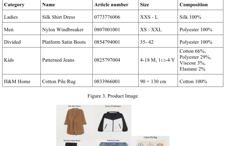
We first collected five homogenous H&M products that are available in ten different countries, which means that the products are strictly identical in terms of size, color, material, and article number (i.e., product ID). Based on its catalog, H&M divided its products into five various departments, including Ladies, Men, Divided, Kids, and H&M Home. The selected products are from each category. These five products are picked from H&M website to guarantee that the data has validity and representativeness. The list of the products and its images are shown in Table 2 and Table 3 respectively.
Table 2. Product Description6
Category Name Article number Size Composition
Ladies Silk Shirt Dress 0773776006 XXS - L Silk 100%
Men Nylon Windbreaker 0807001001 XS - XXL Polyester 100%
Divided Platform Satin Boots 0854794001 35- 42 Polyester 100%
Kids Patterned Jeans 0825797004 4-18 M, 11/2-4 Y
Cotton 66%, Polyester 29%, Viscose 3%, Elastane 2%
H&M Home Cotton Pile Rug 0833966001 90 × 130 cm Cotton 100%
Figure 3. Product Image
13
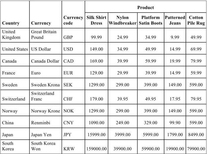
The five products are collected from ten different countries, they are the United Kingdom, the United States, Canada, France, Sweden, Switzerland, Norway, China, Japan, and South Korea. We have to acquire the five product prices from each country in its local currency first. In order to illustrate the international comparison obviously, the price data of the selected productions from ten countries’ independent official websites are demonstrated in Table 3.
Table 3. The Products Prices List in Ten Countries7
Country Currency Currency code Product Silk Shirt Dress Nylon Windbreaker Platform Satin Boots Patterned Jeans Cotton Pile Rug United Kingdom Great Britain Pound GBP 99.99 24.99 34.99 9.99 49.99
United States US Dollar USD 149.00 34.99 49.99 14.99 69.99
Canada Canada Dollar CAD 169.00 39.99 59.99 19.99 79.99
France Euro EUR 129.00 29.99 39.99 14.99 59.99
Sweden Sweden Krona SEK 1299.00 299.00 399.00 149.00 599.00
Switzerland
Switzerland
Franc CHF 179.00 39.95 49.95 17.95 79.95
Norway Norway Krone NOK 1299.00 299.00 399.00 149.00 599.00
China Renminbi CNY 1090.00 249.00 329.00 99.90 599.00
Japan Japan Yen JPY 15999.00 3999.00 5999.00 1799.00 8499.00
South Korea
South Korea
Won KRW 159000.00 39900.00 59900.00 19900.00 79900.00
After collecting them, it is necessary to convert them into a common currency, the single currency of euro has been chosen. Before expressing the prices in euro, we have to gather exchange rate of each country to euro from an official currency converter webpage to ensure its accuracy. The exchange rates were picked in February 2020 with the same time period we collected the prices of the products. This is in order to make them consistent since the newest prices we collected on H&M websites are published thus far in February 2020. The exchange rates are presented in Table 4.
The prices of the products converted into euros in ten different countries are listed in Table 5. The average price for each product is calculated and presented in the last column. Based on the table, it is not difficult to observe that the United States, Switzerland, China, and South Korea have their prices above their average for both Silk Shirt Dress and Nylon Windbreaker. For Platform Satin Boots, we have the same countries list that has their prices above the mean but China changed to Japan in this case. There are only three countries that have their prices above the average for Patterned Jeans, they are France, Switzerland, and South Korea.
14
Table 4. Exchange Rate8
Country Currency Euro Equivalent Currency per Euro
United Kingdom Great Britain Pound 1.203 0.831
United States US Dollar 0.925 1.080
Canada Canada Dollar 0.698 1.432
France Euro 1.000 1.000
Sweden Sweden Krona 0.095 10.566
Switzerland Switzerland Franc 0.942 1.061
Norway Norway Krone 0.099 10.065
China China Yuan/Renminbi 0.132 7.563
Japan Japan Yen 0.008 118.731
South Korea South Korea Won 0.001 1286.702
For the last product Cotton Pile Rug, Switzerland and the three Asian countries have higher prices above the average. To conclude the results based on Table 5, the United States, Switzerland, and the three Asian countries usually have higher prices compared to the other five countries, after expressing in a common currency9. Most western countries such as the United Kingdom, Canada, Sweden, and Norway display prices at relatively low levels.
According to the subsection of 2.3.1 (Trade Barriers), we would expect South Korea, China, and Japan have the highest common-currency price levels due to they have relatively higher rates of tariff compared to other Westerns. This has just been confirmed, but it can partially explain why H&M sold its products expensively in these countries since the United States and Switzerland are not in the list of the countries with the highest tariff rate. Other factors may affect the firm’s price-setting strategies for instance, productivity and VAT.
If LOP and PPP hold true, the prices of the products from each country should be equivalent to its mean prices after converting into a common currency. However, based on Table 5 we examined that China has 3 out of 5 product prices that are above its average, while the United States has the prices which are below average in 3 out of 5 cases. This shows strong deviations on the prices, indicating that the LOP and the PPP do not hold for the commodities of H&M from a data point of view. However, we will examine whether PPP is held in a statistical way by using empirical models in the subsection of 4.3 (Empirical Findings).
8 X-rates - http://www.x-rates.com
9 We did a test which shows that the countries for each product above the average are the same
as changing the common currency from euro to another common currency, for instance, US dollar (see Appendix, Table A1). This indicates that we removed the effect of different currencies being felt on the prices.
15
Table 5. The Products Prices List in Common Currency
Country Currency Product Silk Shirt Dress Nylon Windbreaker Platform Satin Boots Patterned Jeans Cotton Pile Rug
United Kingdom Euro 120.29 30.06 42.09 12.02 60.14
United States Euro 137.83 32.37 46.24 13.87 64.74
Canada Euro 117.96 27.91 41.87 13.95 55.83 France Euro 129.00 29.99 39.99 14.99 59.99 Sweden Euro 123.41 28.41 37.91 14.16 56.91 Switzerland Euro 168.62 37.63 47.05 16.91 75.31 Norway Euro 128.60 29.60 39.50 14.75 59.30 China Euro 143.88 32.87 43.43 13.19 79.07 Japan Euro 127.99 31.99 47.99 14.39 67.99
South Korea Euro 159.00 39.90 59.90 19.90 79.90
Mean Price 135.66 32.07 44.60 14.81 65.92
In the subsection of 2.3.3 (Value-added tax), we comprehended the important role of VAT plays in the price-settings. When determining the global cost for the macroeconomic calculation of a measure, the relevant prices to be taken into account are the prices excluding VAT. The price without VAT is also called VAT exclusive, a price to which tax is yet to be added to arrive at the final cost. To calculate prices deducting from the VAT by using the equation (4).
𝑃𝑟𝑖𝑐𝑒!"# = 𝑃𝑟𝑖𝑐𝑒!"# × (1 − 𝑉𝐴𝑇) (4) where 𝑃𝑟𝑖𝑐𝑒!"# is the original product prices we collected from the H&M catalog converted in euros, which is the numeric in Table 5. 𝑃𝑟𝑖𝑐𝑒!"# is the prices in Table 5 excluding the VAT
rate.
The standard rate of VAT applied in ten countries is illustrated in Figure 4. The highest VAT rate of 25% is distributed in Sweden and Norway while the lowest VAT rate of 5% goes to Canada. In general, the VAT rate applied in Western countries is apparently higher than those in Asian countries. The prices after deducting the VAT rate is shown in Table 6.
From Table 5 and Table 6, we noticed that there are no significant changes in the countries that have their prices above the average for each product we depicted previously compared to the prices without VAT, indicating that the strong deviations from PPP still exist.
16
Figure 4. The VAT Rate Distribution in Ten Countries10
Table 6. The Products Prices List in Common Currency without VAT
Country Currency Product Silk Shirt Dress Nylon Windbreaker Platform Satin Boots Patterned Jeans Cotton Pile Rug
United Kingdom Euro 96.23 24.05 33.67 9.61 48.11
United States Euro 124.04 29.13 41.62 12.48 58.27
Canada Euro 112.06 26.52 39.78 13.26 53.04 France Euro 103.20 23.99 31.99 11.99 47.99 Sweden Euro 92.55 21.30 28.43 10.62 42.68 Switzerland Euro 155.63 34.74 43.43 15.61 69.51 Norway Euro 96.45 22.20 29.63 11.06 44.48 China Euro 123.88 28.30 37.39 11.35 68.08 Japan Euro 117.75 29.43 44.15 13.24 62.55
South Korea Euro 143.10 35.91 53.91 17.91 71.91
Mean Price 116.49 27.56 38.40 12.71 56.66
17
An example of a comparison of the price difference for the product, Silk Shirt Dress, is presented in Figure 5. Norway and Sweden have the largest price discrepancies due to the fact that they have the highest VAT rate (25%) among others.
Figure 5. The Silk Shirt Dress Price Distribution
Thus far, price deviations from PPP do exist and PPP does not prevail based on the data point of view. This conclusion remains unchanged even if we excluded the effect of VAT on the prices. It is also interesting to see which currencies are “too low” or “too high” using H&M Index compared with the Big Mac Index illustrated in Table 1. In other words, we try to figure out if the countries that have their currencies undervalued or overvalued against the US dollar are the same as if we use the Big Mac Index. The first H&M Index is computed based on the product, Silk Shirt Dress. Notice that since we are not interested in testing the effects of exchange rates on prices, the actual dollar exchange rates used to compute the H&M Index are the same as reckoned for the Big Mac Index, that is exchange rates listed in Table 1. Figure 6 displays the comparison of the H&M Index (Silk Shirt Dress) with the Big Mac Index against the US dollar.
Figure 6. Comparison of The H&M Index (Silk Shirt Dress) with The Big Mac Index
To compare with the two indexes, we observe that the tendencies of the changes in the currencies are the same in most countries. The sign of the undervaluation or overvaluation is fairly similar. Goods and services are most expensive in Switzerland examined by both of the
18
indexes. Canada is the cheapest country measured by the H&M index while China is the cheapest nation illustrated by the Big Mac Index. By this measure, we must highlight that Norway and China have the opposite signs which indicate that the indexes give two completely different results of measuring the standard of living by looking at the PPP exchange rate. Meanwhile, the degree of under/over valuation of the currency tends to be small for H&M. This can be explained by differences in demand between countries. Exchange rates do not fully reflect the relative worth of money in different countries. Goods and services will be subjected to their own supply and demand depending on local conditions, such as consumer preferences. Different price-setting strategies across countries may depend on the difference in national consumer behavior observable to the seller. Probably, consumers in one country, for example, China, have a stronger preference for say ladies’ clothing than consumers in other countries, such as Norway, which should be revealed in the country-specific price effects for product groups. In this case, market segmentation will be based on different demand elasticities for product groups, resulting in markups differencing by country and product group. This refers to pricing to market (PTM) that firms try to discriminate between national markets according to the national differences in price elasticity of demand. Empirical studies have shown the clear existence of this practice in manufacturing trade (Raman & Chatterjee, 1995). Silk Shirt Dress might be sold more expensively in China due to strong consumer demand, which also explained why Big Mac sold at a cheaper price, leading to an undervalued currency on the Big Mac Index. On the other hand, the H&M Index has its weaknesses. The products reckoned for the Index are not suitable consumer goods by which to measure general well being. They are considered durable goods, rather than consumer goods. In other words, too few of them are bought because of market segments for the given product is key to attracting customers. For instance, women are the primary consumers of Silk Shirt Dresst, however, Big Mac is the one suitable for all customers in terms of men, women as well as kids. Based on biased demand and consumer preference differentiation, the degree of under/over valuation of the currency tends to be small for H&M can be explained.
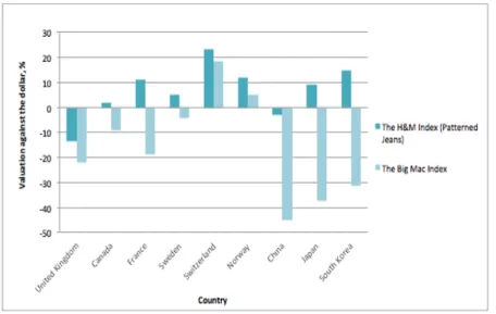
If we change the product from Silk Shirt Dress to Patterned Jeans in order to illustrate the second H&M Index, the results of the currencies against the US dollar are completely different from that of the previous H&M Index. The comparison of the new H&M Index (Patterned Jeans) with the Big Mac Index is shown in Figure 7. The signs are opposite in most countries indicating that where the Big Mac is expensive, the H&M product is cheap. Switzerland is still the most expensive nation, but the cheapest country is denoted by the United Kingdom in this case. The Index of the other three products and their comparisons with the Big Mac Index are listed in the Appendix.
Margolf (2011) offers an analysis of two unconventional indexes developed by The Economist, the well-established Big Mac Index (BMI) and the new and innovative Wiggle Room Index (WRI) in order to figure out which of the indexes is more reliable. The author argues that both have shortcomings and the BMI is applicable for countries that McDonald’s operates regardless of their current state of development, while the WRI can be exclusively used for having a look at emerging markets. Moreover, the author points out that investors are not advised to rely on these indexes, although the indexes’ intentions are good, especially when it comes to making difficult topics more intelligible for readers who are not so much involved in economics. In general, these kinds of indices seem to produce different results so that it is maybe not the best idea to rely too much on a single one. The H&M Index is a complement to the existing indices that can be used to determine if a currency is over-/undervalued though the weaknesses remain. Furthermore, it is the one based on the clothing sector. The sector is important in economic and social terms, in the short-run by providing incomes, jobs, especially for women,
19
and foreign currency receipts and in the long-run by providing countries the opportunity for sustained economic development11.
Figure 7. Comparison of The H&M Index (Patterned Jeans) with The Big Mac Index
4.2 Empirical Models
In this subsection, two regression models will be established and its functional mechanisms will be discussed. In the first place, a quantitative log-linear regression model is established based on the previous study provided by Hassink and Schettkat (2001). The five homogeneous products in ten different countries have been collected, which contains 50 observations in total. The first empirical model is found by the following procedure. First set price variable P as (𝑃!,!∗ ), where i refers to the five products (i = 1, ..., 5) and c is the ten countries (c = 1, ..., 10). The price variable P is denoted in Table 5. Then the average common-currency price of item i in the selected countries will be calculated and store it as (𝑃!,∗). Thus, we have five mean prices. Finally, we take a natural logarithm (ln) of the prices of the products in each country and of the mean prices in order to interpret the result as a percentage difference. The first empirical model is shown in model (1).
ln(𝑃!,!∗ ) − ln(𝑃!,∗) = 𝛼! + 𝛼!𝐷!" + 𝛼!𝐷!" + ⋯ + 𝛼!𝐷!"#"$ + 𝑢!,! (1)
The predicted variable represents the percentage difference between the price of the product i in the c-th country and the mean price (𝑃!,∗). If the predicted variable in country c, ln(𝑃!,!∗ ) − ln(𝑃!,∗) equals 0.5, then the price level for each product in the c-th country is thus on average 50% higher relative to the mean price for all countries. The control variables are dummy variables of the selected countries. 𝐷! equals 1 if the observation comes from country c. u is a stochastic
error term assumed to be normally distributed. Notice that since we have ten countries, we have introduced only nine dummy variables to avoid falling into a dummy-variable trap (i.e., the situation of perfect collinearity). Here we are treating South Korea as the reference country. This can trace to South Korea is one of the selected markets that display common-currency prices at relatively higher levels and is the one who has the highest tariff rate. Therefore, it is interesting to see how much the price levels of the other countries differ from the value of South Korea.
11 Overseas Development Institute -
20
Model one is to test whether the coefficients of dummies in all countries are zero. If the coefficient estimates are not equal to zero, indicating that the common-currency prices for specific products are not the same in every country. Thus, PPP definitely does not prevail if we reject the null hypothesis.
Afterwards, we want to investigate which variables have a greater impact on the price discrepancies. As mentioned in the subsection of 2.3 (PPP deviation puzzle), the following factors are considered as explanatory variables to examine the affection on price settings. They are Trade barriers (tariff), Non-tradable inputs (productivity and labor cost), and Value-added tax (VAT). Both tariff and VAT are a kind of tax system, the two variables we are interested to test are productivity and VAT. Take these two factors into account in order to compare estimated empirical results to results from a previous study. In this case, the second empirical model, which is shown in model (2), is built to test if productivity and/or VAT has a significant impact on the price difference.
ln(𝑃!,!∗ ) − ln(𝑃
!,∗) = 𝛼! + 𝛼!𝐷!" + 𝛼!𝐷!" + ⋯ + 𝛼!𝐷!"#$%& + 𝜒!𝑃𝑟𝑜𝑑𝑢𝑐𝑡𝑖𝑣𝑖𝑡𝑦! + 𝜒!𝑉𝐴𝑇! + 𝑣!,! (2)
Productivity and VAT will be considered by software as dummy variables, thus we have introduced only seven dummies to avoid the situation of perfect collinearity. South Korea will still act as the benchmark. There is a linear relationship between the two explanatory variables and the predicted variable due to the fact that there is only one value from each explanatory regarding each country. In other words, the coefficient estimates of these two variables (𝜒! and
𝜒!) are located in the range -1 to 1. Based on the theories depicted in the subsection of 2.3 (PPP
deviation puzzle), increase in productivity and VAT tend to have positive impacts on prices, therefore, we would expect the sign of both 𝜒! and 𝜒! to be positive and at the same time the
estimated coefficients are expected to be significantly different from zero.
The data on productivity in 2019 gathered from the World Bank, which is GDP per person employed (constant 2011 PPP $). This is the most recent dataset provided by the World Bank. It can contribute to a differentiation throughout the time horizon to some extent since other necessary measures of analysis such as prices of the products and VAT are from 2020. However, it is not possible to collecting data on productivity after 2019 due to the total GDP produced for a whole year of 2020 can not be measured thus far. The illustration of the productivity of the selected countries is demonstrated in Figure 8.
Figure 8. Ten Countries Productivity12
21
4.3 Empirical Findings
The two log-linear regression models are estimated by applying the ordinary least square method (OLS). The regression outputs will be analyzed in detail in order to make a final judgment on PPP. Moreover, we will examine if both productivity and VAT are positively related to the price level. Afterwards, we make a comparison of the empirical results to results from a previous study to examine whether they display similar outcomes. Further analysis is necessary if the results are not the same.
The regression output for the first empirical model is shown in Table 7. Notice that we have chosen South Korea as the reference country. The intercept (constant) is the estimated coefficient of South Korea and the other coefficients represent how much the intercept values of the other countries differ from the intercept value of South Korea. The sum of the two coefficients gives the actual value of the intercept for the selected country. The coefficient estimate of South Korea is 0.232, that is that price in South Korea is 23.2% higher than the average. The coefficient estimate of the United Kingdom is -0.340, that is that price in the UK is 34% lower than those in South Korea. In other words, the price in the UK is about 10.8% low compared to the average.
The actual output shows that South Korea has the highest price level (+26.1%)13 and Sweden
has the lowest price level (-10.8%)14. The range of the country effects is about 37 percentage
points, which is a considerably wide range. The value of R-squared suggests that the model explains about 80.57% of the inter-country price variation. This indicates that the selected countries have fairly the right of interpretation on price discrepancies.
The first empirical model is to test whether common-currency prices for specific products are the same in every country. That is, the coefficients for all country dummies are zero. Under the null hypothesis, the country effect is zero, indicating that no common-currency price differences for the same good between countries. The alternative hypothesis states a country-specific effect exists, which may differ across countries. Model (3) represents both null and alternative hypotheses.
𝐻!: 𝛼.,! = 0, ∀ c VS. 𝐻!: 𝛼.,! ≠ 0 (3)
With 9 degrees of freedom in numerator and 40 degrees of freedom in denominator, the critical value of F at a 5% significance level equals 2.12. Reject the null hypothesis if F-statistic is greater than 2.12. With F=18.44, 18.44 > 2.12, we reject the null hypothesis and conclude that at least one of the dummy variables are statistically significantly different from zero. This indicates that the country-specific effect does exist, identical H&M products do not sell at the same price in every country when expressed in a common currency. Based on the empirical result, we can conclude that PPP definitely does not hold for H&M and in the mean while the LOP is also violated.
The result of the second empirical model is illustrated in Table 8. The estimated country coefficients change extremely and some of them alter signs. The ranking of the countries as well as the difference between the highest and lowest price level have been amended suggesting that differences in non-tradable inputs and VAT may affect price settings. The R-squared of 0.8057 does not increase if we include two explanatory variables such as productivity and the VAT.
13 If D
South Korea switches from 0 to 1, price level will increase bye(0.232) -1 percentage. 14 If D
22
Table 7. The Regression Output for Model One Model (1)15 Dependent variable: ln(𝑃!,!∗ ) − ln(𝑃!,∗) Coefficients t-values 1 United Kingdom -0.340*** -8.95 2 United State -0.236*** -6.12 3 Canada -0.345*** -9.07 4 France -0.293*** -7.71 5 Sweden -0.346*** -9.09 6 Switzerland -0.092** -2.43 7 Norway -0.304*** -8.01 8 China -0.207*** -5.45 9 Japan -0.228*** -6.01 Constant 0.232*** 8.62 summary statistics # dummy variables 9 F-test 18.44 R-squared 0.8057 Adj. R-squared 0.7621 SSR 0.1448 N 50
***p-value< 0.01 **p-value< 0.05 *p-value< 0.1
15 ln(𝑃
23
Table 8. The Regression Output for Model Two Model (2)16 Dependent variable: ln(𝑃!,!∗ ) − ln(𝑃 !,∗) Coefficients t-values 1 United Kingdom -2.236*** -6.95 2 United State -1.187*** -7.05 3 Canada 0.165** 2.19 4 France -2.511*** -6.79 5 Sweden -3.463*** -6.77 6 Switzerland -0.432*** -5.39 7 Norway -4.096*** -6.69 8 China - - 9 Japan - - Constant -2.982*** -6.26 Productivity 2.12E-05*** 6.61 VAT 0.168*** 6.27 summary statistics # dummy variables 7 F-test 18.44 R-squared 0.8057 Adj. R-squared 0.7621 SSR 0.1448 N 50
***p-value< 0.01 **p-value< 0.05 *p-value< 0.1
16 ln(𝑃