IN
DEGREE PROJECT MATHEMATICS, SECOND CYCLE, 30 CREDITS
,
STOCKHOLM SWEDEN 2016
Importance Sampling for
Least-Square Monte Carlo
Methods
ILYAS AHMED
KTH ROYAL INSTITUTE OF TECHNOLOGY SCHOOL OF ENGINEERING SCIENCES
Importance Sampling for Least-Square
Monte Carlo Methods
I L Y A S A H M E D
Master’s Thesis in Mathematical Statistics (30 ECTS credits) Master Programme in Applied and Computational Mathematics (120 credits)
Royal Institute of Technology year 2016 Supervisor at Swedbank: Per Fust Supervisor at KTH: Boualem Djehiche Examiner: Boualem Djehiche
TRITA-MAT-E 2016:64 ISRN-KTH/MAT/E--16/64-SE
Royal Institute of Technology
SCI School of Engineering Sciences
KTH SCI
SE-100 44 Stockholm, Sweden URL: www.kth.se/sci
Abstract
Pricing American style options is challenging due to early exercise opportunities. The conditional expectation in the Snell envelope, known as the continuation value is ap-proximated by basis functions in the Least-Square Monte Carlo-algorithm, giving robust estimation for the options price. By change of measure in the underlying Geometric Brownain motion using Importance Sampling, the variance of the option price can be reduced up to 9 times. Finding the optimal estimator that gives the minimal variance requires careful consideration on the reference price without adding bias in the estima-tor. A stochastic algorithm is used to find the optimal drift that minimizes the second moment in the expression of the variance after change of measure. The usage of Im-portance Sampling shows significant variance reduction in comparison with the standard Least-Square Monte Carlo. However, Importance Sampling method may be a better alternative for more complex instruments with early exercise opportunity.
Sammanfattning
Prissättning av amerikanska optioner är utmanande på grund av att man har rätten att lösa in optionen innan och fram till löptidens slut. Det betingade väntevärdet i Snell envelopet, känd som fortsättningsvärdet approximeras med basfunktioner i Least-Square Monte Carlo-algoritmen som ger robust uppskattning av optionspriset. Genom att byta mått i den underliggande geometriska Browniska rörelsen med Importance Sampling så kan variansen av optionspriset minskas med upp till 9 gånger. Att hitta den optimala skattningen som ger en minimal varians av optionspriset kräver en noggrann omtanke om referenspriset utan att skattningen blir för skev. I detta arbete används en stokastisk algoritm för att hitta den optimala driften som minimerar det andra momentet i uttrycket av variansen efter måttbyte. Användningen av Importance Sampling har visat sig ge en signifikant minskning av varians jämfört med den vanliga Least-Square Monte Carlo-metoden. Däremot kan importance sampling vara ett bättre alternativ för mer komplexa instrument där man har rätten at lösa in instrumentet fram till löptidens slut.
Importance Sampling för Least-Square
Monte Carlo-metoder
Acknowledgements
I take this opportunity to thank professor Boualem Djehiche at KTH for his excellent guidance and feedback. I would also like to thank Per Fust and Bengt Pramborg at Swedbank for their valuable guidance for writing this thesis. Finally, I would like to thank my family for their constant support for higher education.
Contents
Abstract i
Sammanfattning ii
Acknowledgements iii
List of Figures vi
List of Tables vii
Abbreviations viii
1 Introduction 1
1.1 Background . . . 1
1.2 Previous Studies . . . 2
1.3 Aim of this Thesis . . . 2
2 Mathematical Background 4 2.1 American Options . . . 4
2.1.1 Snell-envelope in discrete time. . . 5
2.2 Monte Carlo Methods . . . 6
2.2.1 Principal Aim . . . 7
2.2.2 Importance Sampling. . . 7
2.3 Exponential Change of Measure . . . 9
3 Least Square Monte Carlo 11 3.1 The LSM Approach . . . 11
3.1.1 Scenario Generation . . . 12
3.2 Basis Functions . . . 13
3.2.1 Second order polynomial . . . 14
3.2.2 Laguerre Polyonmials . . . 15
3.3 Convergence of the LSM algorithm . . . 16
4 Implementing the IS-LSM Algorithm 17 4.1 Expectation and the Likelihood Ratio . . . 17
v
4.2 IS-LSM Algorithm . . . 19
4.2.1 Convergence of the IS-LSM algorithm . . . 20
4.2.2 Stochastic Approximation for Optimal Drift . . . 21
5 Results 24
6 Discussion 34
A Essential supernum 36
List of Figures
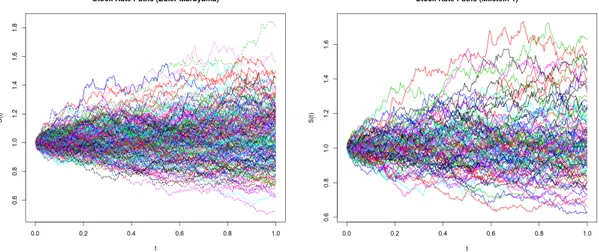
3.1 A realization of 200 stock rate paths using Euler-Maruyama scheme (left) and Millstein 1 scheme (right) over 251 trading days with S0 = 1, r =
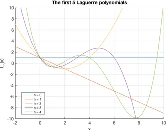
0.02, = 20%and T = 1. . . 12 3.2 The first 5 Laguerre polynomials . . . 15
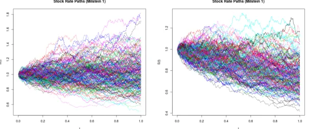
4.1 A realization of 200 stock rate paths with drift ✓ = 0 (left) and with drift ✓ = 1.6 (right) over 251 trading days with S0 = 1, r = 0.02, = 20%
and T = 1. . . 18
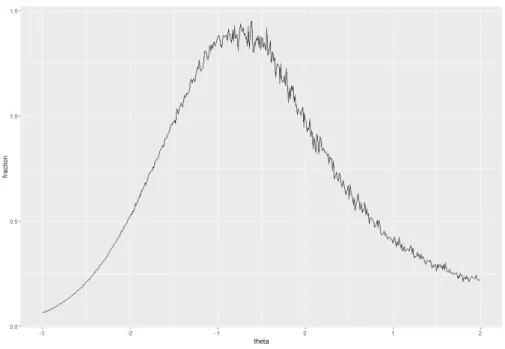
5.1 A brute-force plot of V0IS-LSM
V0LSM as a function of ✓ with K = 50 and = 50%. 25
5.2 Convergence of put option using standard LSM (left) and IS-LSM (right) with 2nd-order polynomials and sample size of n = 5000. The pricing
parameters here are S0 = 50, K = 50, r = 0.02, = 10% and T = 1. . . . 28
5.3 Convergence of put option using standard LSM (left) and IS-LSM (right) with a sample size ofwith 2nd-order polynomials and sample size of n =
5000. The pricing parameters here are S0 = 50, K = 50, r = 0.02,
= 50% and T = 1. . . 28 5.4 Convergence of put option using standard LSM (left) and IS-LSM (right)
with 2nd-order polynomials and sample size of n = 5000. The pricing
parameters here are S0 = 50, K = 54, r = 0.02, = 10% and T = 1. . . . 29
5.5 Convergence of put option using standard LSM (left) and IS-LSM (right) with 2nd-order polynomials and sample size of n = 5000. The pricing
parameters here are S0 = 50, K = 54, r = 0.02, = 50% and T = 1. . . . 29
5.6 Convergence of put option using standard LSM (left) and IS-LSM (right) with Hermite-polynomials and a sample size of n = 5000. The pricing parameters here are S0 = 50, K = 50, r = 0.02, = 10% and T = 1. . . . 30
5.7 Convergence of put option using standard LSM (left) and IS-LSM (right) with Hermite-polynomials and a sample size of n = 5000. The pricing parameters here are S0 = 50, K = 50, r = 0.02, = 50% and T = 1. . . . 30
5.8 Convergence of put option using standard LSM (left) and IS-LSM (right) with Hermite-polynomials and a sample size of n = 5000. The pricing parameters here are S0 = 50, K = 54, r = 0.02, = 10% and T = 1. . . . 31
5.9 Convergence of put option using standard LSM (left) and IS-LSM (right) with Hermite-polynomials and a sample size of n = 5000. The pricing parameters here are S0 = 50, K = 54, r = 0.02, = 50% and T = 1. . . . 31
5.10 Reference ratio vs ✓ 2 [ 1.17, 1.15] with K = 56 and = 50%. . . 32
List of Tables
5.1 Strike price K = 50 with 2nd-order polynomial . . . 25
5.2 Strike price K = 52 with 2nd-order polynomial . . . 26
5.3 Strike price K = 54 with 2nd-order polynomial . . . 26
5.4 Strike price K = 56 with 2nd-order polynomial . . . 26
5.5 Strike price K = 50 with Hermite-polynomials. . . 27
5.6 Strike price K = 52 with Hermite-polynomials. . . 27
5.7 Strike price K = 54 with Hermite-polynomials. . . 27
5.8 Strike price K = 56 with Hermite-polynomials. . . 27
5.9 Optimal ✓ using second order polyomials. . . 33
5.10 Optimal ✓ using using Hermite-polynomials. . . 33
Abbreviations
DynP Dynamic Programming GBM Geometric Brownian Motion IS Importance Sampling
LSM Least-Squares Monte Carlo
IPA Infinitesimal Perturbation Analysis SA Stochastic Approximation
Chapter 1
Introduction
Pricing methods of American style options has been well studied and there exists several different methods that are robust in a sense that they reflect the relevant price. Unlike the case of European options, where the price is deterministic by the Black & Scholes pricing formula, there is no closed form pricing model for American style options due to the early exercise opportunity. Pricing this kind of instruments requires numerical methods or Monte Carlo simulation in order to make relevant approximations of its price at time t = 0. This thesis will focus on efficient Monte Carlo methods for pricing an American put option. We will implement a modification of the well known algorithm developed by Longstaff & Schwartz by using importance sampling in order to get a variance reduction for the estimated price.
1.1 Background
Considering a one dimensional case of an underlying asset, the payoff function of the American option written on the asset is dependent on the strike price K of the written contract. Unlike the European equivalents, the American style options have early exercise opportunity at some time ⌧ < T . These options with payoff function f are priced as:
V0 = sup ⌧2T[0,T ]
E[e r⌧f (⌧, S
⌧)]. (1.1)
The solution to (1.1) is an optimal stopping problem and has by usage of Dynamic Programming (DynP), a well-known solution. However, the outcome of the solution is not in closed form and V0 needs to be priced by either numerical methods or Monte
Carlo simulation, by the rules of the DynP solution. Longstaff & Schwartz introduced 1
2 a regression based approach to approximate (1.1). This is known as the Least-Square Monte Carlo algorithm or just simply LSM. It approximates the conditional expectations occurred in the optimal stopping problem with well behaved basis functions such that the price of the option at time t = 0 can be priced. However, the LSM-algorithm can give less accurate estimates if the strike prices and volatilities of the underlying asset are large. For this, efficient improvements of the LSM algorithm has to be done by means of change of measure in the underlying process.
1.2 Previous Studies
Studies of pricing American style options are well presented in several literature. Cox in [4] used the binomial tree methods for pricing these options. There are also trinomial trees and finite difference method for estimating the option price. The Longstaff & Schwartz method in [9] is based on Least-Square Monte Carlo method which is an efficient and yet simple method due to that it approximates the conditional expectation using basis functions. Moreni in [10] introduced an Importance Sampling (IS) approach for the LSM algorithm using American basket put options. The fact that LSM is only relevant for realizations that are in-the-money, the Monte Carlo estimate can deviate from the "true" value. The idea of implementing IS together with LSM is to make a change of drift in the underlying process and thereby getting more paths in-the-money. Moreni [10] used this technique with help of convergence ratio and European-derived criterion to find the optimal change of drift ✓ of the underlying process.
1.3 Aim of this Thesis
The aim of this thesis is to consider the LSM algorithm together with IS studied in Moreni [10], but with slightly different approaches. Here we focus on a simple American put option and try to find the optimal drift of the underlying process after change of measure. The method to be used is the exponential twisting method and we want to solve the optimization problem that minimizes the optimal drift ✓ as presented by Glasserman in [6]. The quantity of interest is that we have a convex function H(✓) which is the second moment of the IS estimator and want to solve:
H(✓⇤) = min
✓2RH(✓) (1.2)
We combine this study by using both stochastic approximation (SA) and infinitesimal perturbation analysis (IPA) as presented by Graham in [7] and Su in [11]. The goal is
3 to implement an algorithm that finds the value of the drift that gives a better variance reduction compared to standard LSM. The results of these methods then compared with findings in Moreni.
In Chapter 2, the mathematical background is introduced for setting up the necessary framework. In Chapter 3, the LSM algorithm is presented followed by the implementation of IS and the optimal drift in Chapter 4. Chapter 5 presents the results followed by conclusions in Chapter 6.
Chapter 2
Mathematical Background
This chapter presents the necessary mathematical background that is needed for later chapters when implementing the desired modified LSM algorihm. To begin with, we assume that our market model exists from time t = 0 to t = T only. Introduce a probability space (⌦, P, F, (Ft)t2[0,T ]), where F is a -algebra with filtration (Ft)t2[0,T ].
The probability measure P is the standard measure that is relevant when changing to the risk-neutral measure during pricing.
2.1 American Options
Definition 2.1. An American put option with maturity T , strike price K and payoff function f(t, S(t)) = max(K S(t), 0) is a contingent claim that can be exercises at any time t T .
At time to maturity T , the price of the option is V (T, S(T )) = f(T, S(T )) and in order to preclude arbitrage for the filtration (Ft)t2[0,T ], the price has to satisfy the condition
V (t, S(t)) f (t, S(t)) for t 2 [0, T ]. Until the exercise moment, the option satisfies the partial differential equation:
rs@V (s, t) @s + 1 2 2s2@2V (s, t) @s2 rV (s, t) + @V (s, t) @t = 0 (2.1)
The general rule is that the holder should exercise the option as soon as the price V (S(t), t) = f (S(t), t). During this time the equality in (2.1) becomes an inequality due to the fact that V (S(t), t) may not represent the value process of a strategy after the optimal exercise. The price of the American put satisfies the following boundary conditions:
V (S(T ), T ) = max(K S(T ), 0) (2.2)
5 lim s!0V (s, t) = K (2.3) and lim s!1V (s, t) = 0 (2.4)
Note that at t = T , by equation (2.2) the price of the option is given by the standard Black & Scholes formula for European put (given that there are no dividend payments) option that is:
VEUput = Ke rT ( d2) S0 ( d1) (2.5)
where is the standard normal cumulative distribution function and d1 and d2 are given
by: d1 = log⇣S0 K + T (r + 2 2 ) ⌘ p T ; d2 = d1 p T (2.6)
The extreme simplification by "elimination of risk" by the Black & Scholes formula does not require the knowledge on how the underlying asset behaves prior to time T . This is however not fully applicable for the American style options due to early exercise opportunity. A concrete and relevant aspect of the American style options is presented by the Snell-envelope discussed next.
2.1.1 Snell-envelope in discrete time
In this thesis, we approximate the original stopping problem in continuous time with the stopping problem in discrete time as described in [2] and [5]. This results an optimal stopping time that differs from the original optimal stopping time. Let (Zj)Nj=0 be an
adapted payoff process with Z0, Z1, ..., ZN being square integrable random variables and
let T = {⌧0, ⌧1, ..., ⌧N} [ R+ be set of optimal stopping times. As the objective is to
compute equation (1.1), we have to solve the optimal stopping problem given by the Snell-envelope.
Definition 2.2. Let (⌦, P, F) be a probability space. The adapted process (Vj)Nj=0 is
the Snell envelope on the process (Zj)Nj=0 if:
1. V is a super P-martingale 2. Vj Zj for all j = 0, ..., N
6 In other words, the value process Vj of an American option can be constructed with the
Snell envelope using N time steps with filtration (Fj)j 0 such that:
Vj = ess sup
⌧2T E [Z⌧|Fj
] , for j = 0, ..., N (2.7)
where ess sup denotes the essential supernum (see Appendix for details). The resulting DynP principle can be written as:
Vj = 8 < : ZN, j = N max{Zj,E[Vj+1|Fj]}, 0 j N 1 . (2.8)
The sequence of stopping times is given by: 8 > > > < > > > : ⌧0= inf{k 0|Vk= Zk} ^ N ⌧j = inf{k ⌧j 1|Vk= Zk} ^ N ⌧j+1 ⌧j (2.9)
which then obeys the DynP scheme (in discrete time) in terms of the optimal stopping times ⌧j: 8 < : ⌧N = N ⌧j = j1{Zj E[Zj+1|Fj]}+ ⌧j+11{Zj<E[Zj+1|Fj]}, 0 j N 1 (2.10) This formulation in terms of the optimal stopping rules place a central role in the least square regression method in the LSM algorithm. Note that ⌧0 < ⌧1 < ... < ⌧N and that
inf in (2.9) is indeed a min since we are dealing with discrete time. The adapted payoff process (Zj)Nj=0 is given by the American put option given in Definition 2.2i.e:
Zj = f (j, Sj) (2.11)
where underlying model is assumed to be a (Fj)-Markov chain for some Borel function
f (j,·) (see [3] for more details). The expectation E[Vj+1|Fj]given in (2.8) is of interest
and is discussed in more detail in the next chapter. We now continue to discuss some important topics in Monte Carlo methods.
2.2 Monte Carlo Methods
Monte Carlo methods are a broad class of algorithms relying on repetitive random sam-pling for obtaining approximate numerical results. The algorithms are used in physical
7 and mathematical problems and are mainly useful when it is impossible to make any standard numerical approximations of a given problem.
2.2.1 Principal Aim
The principal aim for a Monte Carlo methods is related to compute an expectation of the form:
V :=E(h(X)) (2.12)
where X ✓ Rd, i.e. a random variable taking values in d-dimensional real line and the
function h : X ! R is some objective function. The expectation under (2.12) can become complicated to calculate if the objective function has characteristics that implies a large variance. Assuming that this integral is complicated to evaluate both analytically and numerically, we can approximate it by generating a I.I.D. sequence of Xi’s using
pseudo-random number generation and set: 1 N N X i=1 h(Xi) = ˆVN (2.13)
which is the standard Monte Carlo estimator. The estimator ˆVN is unbiased and strongly
consistent as N ! 1 meaning that: ˆ
VN ! V with probability 1 (2.14)
and for large N we can construct a confidence interval for ˆVN by:
ˆ
VN± 1(1 ↵/2)
s
Var( ˆVN)
N
where 1 is the inverse of the cumulative standard normal distribution function.
2.2.2 Importance Sampling
Importance Sampling is attempted to reduce the variance of a standard monte carlo estimator by the change of measure. We know that under P, the standard monte carlo estimator for a function h(X) is:
VN =EP(h(X))⇡ 1 N N X i=1 h(Xi) (2.15)
8 where EP denotes that the expectation is taken under measure P. We now want to
estimate the same expectation under a new measure Q by constructing a sampling average of independent copies of
h(X)dP dQ such that EP[h(X)] = EQ[h(X)dP
dQ]. Assumptions that P << Q is made such that the
likelihood ratio exists. More concrete, if X is a random element with probability density function f under P-measure, then we introduce another probability density function g under Q-measure such that:
f (x) > 0 =) g(x) > 0 for all x 2 R. (2.16) Here, we have that dP = fdx and dQ = gdx . The importance sampling procedure changes the measure to try to give more weight to the important regions of the desired distribution and therefore increasing the efficiency of the sampling. V can then in integral form be represented as:
V = Z
h(x)f (x)
g(x)g(x)dx. (2.17)
Expressing this integral as an expectation, we have the expectation with respect to the density g (i.e. under measure Q) given by:
V =EQhh(X)f (X) g(X) i
=EQ[h(X)w(X)] (2.18)
and its Importance Sampling (IS) estimator is given by: VNIS = 1 N N X i=1 h(Xi)w(Xi). (2.19)
The weight !(X) is known as the Likelihood ratio, or by means of measure theory, the Radon-Nikodym derivative, i.e:
w(X) = dP
dQ =: L. (2.20)
Following from equation (2.18), the importance sampling estimator is unbiased meaning that EQhVˆIS
N
i
= V which yields:
9 Due to this fact, the only quantity of interest is to compare the second moments of the IS and the standard monte carlo estimator:
EQ "✓ h(X)f (X) g(X) ◆2# =EP h(X)2f (X) g(X) . (2.22)
It is desired, but not guaranteed that the variance in the standard Monte Carlo is larger, i.e:
Var [h(X)] Var [h(X)w(X)] .
Since IS can be used for rare-event simulation, the key usage will later on be on the stock-price realizations with more "weight" to important regions.
2.3 Exponential Change of Measure
For a cumulative distribution function F on R, let M(✓) =R1
1e✓xdF (x)be the moment
generating function of F and define the cumulant generating function: (✓) = log
Z 1
1
e✓xdF (x) (2.23)
Introduce ⇥ = {✓ : (✓) < 1} as a non-empty set. Now, for each ✓ 2 ⇥, set: F✓(x) =
Z x 1
e✓u (✓)dF (u); (2.24) where each F✓ is a probability distribution and the set {F✓, ✓2 ⇥} forms an exponential
family of distributions. The transformation from distribution F to F✓ is the exponential
change of measure. Moreover if F has density f then F✓ has the density:
f✓(x) = e✓x (✓)f (x) (2.25)
Example 2.1. Let X1, ..., Xn be i.i.d. with distribution function F . Applying the change
of measure for which Xi’s becomes i.i.d. under distribution F✓, the likelihood ratio of the
transformation is: n Y i=1 dF (Xi) dF✓(Xi) = exp ✓ n X i=1 Xi+ n (✓) ! . (2.26)
Example 2.2. Continuing from example 2.1, we can change the mean of a normal distribution. Let f be the standard normal distribution density and g normal distribution density with mean µ and standard deviation 1. Using the same algebra as from the
10 previous example we simply get:
m Y i=1 f (Zi) g(Zi) = exp µ m X i=1 Zi+ m 2µ 2 ! . (2.27)
If we introduce a grid 0 = t0 < t1 < ... < tm and simulate a Brownian motion given by:
W (tn) = n X i=1 p ti ti 1Zi (2.28)
then the likelihood ratio L for the change of measure adding drift µpti ti 1 to the
Brownian increment over [ti 1, ti]is given by equation (2.27).
Comparing Example 2.1 and Example 2.2, we can conclude that for the standard normal distribution, (✓) = ✓2
2, which is a generalization of change of mean for the normal
distribution. With that said, we can now state the following theorem.
Theorem 2.3. (Girsanov Theorem). Consider the stochastic differential equation in Rd
satisfying the Lipschitz coefficients and driven by the standard Brownian motion: X(t) = X(0) + Z t 0 b(Xs)ds + Z t 0 (Xs)dWs (2.29)
Let (✓s)0sT be an Rd valued measureable adapted process such that:
Z T 0 |✓ s|2ds <1, a.s (2.30) and E exp ⇢Z T 0 ✓s· dWs 1 2 Z T 0 |✓s| 2ds = 1 (2.31)
The probability measure P✓ on (⌦, F
T) defined by the Radon-Nikodym derivative:
dP✓ dP := exp Z T 0 ✓s· dWs 1 2 Z T 0 |✓ s|2ds (2.32)
is equivalent to P. In addition, the process: Wt✓ = Wt
Z t 0
✓sds, 0 t T, (2.33)
is an Brownian motion on (⌦, FT),P✓ and P✓-a.s, for 0 t T ,
Xt= X0+ Z t 0 (b(Xs) + (Xs)✓s) ds + Z t 0 (Xs)dWs✓. (2.34)
Chapter 3
Least Square Monte Carlo
This chapter goes trough the most important aspects of the Longstaff & Schwartz al-gorithm. The procedure is well explained in [9] including a detailed example. This chapter goes briefly trough the procedure of the LSM algorithm and emphasize the most important build-blocks and results of the algorithm.
3.1 The LSM Approach
As mentioned in the previous chapters, the expectation E[Vj+1|Fj]in (2.8) is of interest.
The holder of an American put option with maturity T has to decide whether it is optimal to exercise the option at some time t prior to T . Since the holder does not know the payoff at time t + 1, the optimal stopping problem in terms of the expectation determines the expected value of the option at time t + 1. This expectation is known as the continuation value and the LSM approach approximates this with a set of basis functions in which it then can easily be estimated by simple least square regression. Consider the standard Black & Scholes model that for which the bank account dynamics is given by:
dB(t) = rB(t)dt with B(0) = 1, (3.1)
and the stock price dynamics
dS(t) = µS(t)dt + S(t)dW (t) (3.2)
Under the risk neutral measure Q, the stock price has dynamics:
dS(t) = rS(t)dt + S(t)dW (t)Q (3.3)
12 where r 0, µ 2 R and > 0. This model will be used as the underlying process in the LSM-algorithm. As Longstaff & Schwartz uses the argument of approximating E[Vj+1|Fj]
using basis functions, we can simplify the problem to a least-square regression problem. This means that each continuation value in the Snell-envelope is indeed a least-squares approximation and we can therefore decide whether or not it is optimal to exercise at a given time t = ⌧ prior to t = T .
3.1.1 Scenario Generation
Because we want to numerically simulate (3.3), we need a stochastic approximation for the solution of the underlying process. Considering the stochastic process S driven by the stochastic differential equation:
dS(t) = a(S(t), t)dt + b(S(t), t)dW (t) (3.4) there are several schemes to simulate the above SDE. We set i = ti+1 ti and
approx-imate the SDE by the Euler-Maruyama scheme and Millstein-1-scheme given by: Sti+1 = Sti+ ati + bti p Zi (3.5) and Sti+1 = Sti + ati + bti p Zi+ 1 2b T tibti Z 2 i 1 (3.6)
respectively, where Zi ⇠ N(0, 1). For the case of Geometric Brownian motion, eq (3.3)
has a(S(t), t) = rS(t) and b(S(t), t) = S(t). Stock price realizations are shown in figure
3.1below using both the Euler and Millstein scheme. The Euler scheme has convergence
Figure 3.1: A realization of 200 stock rate paths using Euler-Maruyama scheme (left) and Millstein 1 scheme (right) over 251 trading days with S0 = 1, r = 0.02, = 20%
13 order of O( ). Using Itô’s formula to any twice differentiable C2 function f(S(t), t) and
limiting the expansions of the stochastic integrals, there will be a another term in the approximation whose convergence is of order O( ). Therefore, the Euler Scheme will be incomplete and is compensated with the Millstein 1 Scheme in (3.6) which gives a better approximation of order one in (see [2] for details).
3.2 Basis Functions
The goal is to approximate the conditional expectation appeared in the Snell envelope using basis function. If the payoff function Zt = f (St) of the option has its elements
in the space of square-integrable finite-variance functions L2(⌦,F, Q), then the value of
the option is the maximized values of the discounted cash-flows from the option over all Ft stopping times according to equation (2.9). The conditional expectation is the
continuation value of the option, meaning that if it is larger than the current value at t then we do not exercise at that point of time. In the original paper of Longstaff & Schwartz, the LSM algorithm represents the basis functions as:
F (St) = 1
X
j=0
ajej(St), aj 2 R (3.7)
for some basis function e(·). To implement the LSM algorithm, the approximation of F (St) is done using the first m < 1 basis functions and is denoted as ˆFm(Stk). The
choise of basis functions is entirely arbitrary and can be anything from Hermite, Legendre to Chebyshev polynomials. In this chapter, we will focus on simple second order poly-nomials and Laguerre polypoly-nomials. Since American style options can be approximated by Bermuda-style options, we will discretize the time steps to n = 1, 2, ..., N number of time steps, meaning that the early exercise opportunities are restricted to a finite set. Of course here M should be as large as possible. In the optimal stopping time given in equation (2.9), we let Zk = f (Sk).
When using the LSM algorithm, the option holder chooses at every time tn whether
to exercise or keeping the option alive by comparing the continuation value with the immediate value. Having the approximation of the conditional expectation in hand, the optimal stopping time (⌧[m]
j ) can be expressed recursively by using N⇤ independent
simulated paths with: 8 > < > : ⌧Nn,m,N⇤ = N ⌧jn,m,N⇤ = j1 {Zj(n) ↵ (m,N ⇤) j ·em(X (n) j )} + ⌧j+1n,m,N⇤1 {Zj<↵(m,N ⇤)j ·em(X (n) j )} , 0 j N 1 (3.8)
14 The notion · denotes the inner product in Rm, em is the vector valued function and
↵j(m,N⇤) is given by the estimator:
↵(m,Nj ⇤)= arg min a2Rm N⇤ X n=1 ✓ Zn ⌧j+1n,m,N ⇤ a· e m(X(n) j ) ◆2 . (3.9)
The procedure of the algorithm is presented by following pseudo-code: Algorithm 1 LSM-algorithm
1: for n = 1, ..., N⇤ do
2: Generate realizations of the GBM with N time steps 3: Set ⌧ = N 4: end for 5: fort = N-1,...,1 do 6: for n = 1, ..., N⇤ do 7: Compute a0, ..., aM 8: Set ˆF (t, S(n)(t)) =PM l=0ˆalel(Sn(t)) 9: if V (t, S(n)(t)) F (t, Sˆ (n)(t))then 10: ⌧(n)= t 11: end if 12: end for 13: end for
After optimal stopping time is determined for each path, the price is determined by the averaging over the discounted payoffs. The LSM-algorithm only includes in-the-money paths for estimation which of course makes sense because the value of the payoff function is zero whenever it is out-the-money. However, if the volatility of the underlying process is large or the strike price of the option is high, the out-the-money paths will increase giving less precise estimation (see Chapter 4).
3.2.1 Second order polynomial
The conditional expectation can well be approximated by second order polynomials. For the simple case of American put option, implementations of the LSM-algorithm exists as a library for the R statistical language. In this simple but effective algorithm, the approximation of the continuation value is given by E[Y |X] ⇡ a0+ a1X + a2X2
15
3.2.2 Laguerre Polyonmials
A well known basis function that also is introduced in Longstaff & Schwartz original paper are the Laguerre polynomials defined by:
Ln(x) = n X k=0 ( 1)k k! ✓ n k ◆ xk (3.10)
and it is fortunately enough to only use the first four terms of the series [9], i.e: L0(x) = 1 L1(x) = x + 1 L2(x) = 1 2 x 2 4x + 2 L3(x) = 1 6 x 3+ 9x2 18x + 6
Figure3.2 shows the first 5 Laguerre polynomials plotted between 2 x 10.
Figure 3.2: The first 5 Laguerre polynomials
In, [9] it is emphasized that in order to avoid computational underflows during pricing, it is recommended to normalize the cash-flows by dividing all cash flows and prices by the strike price and weighting the Laguerre polynomials by exp ( x/2) resulting in Hermite polynomials: Hn(x) = exp( x/2) ex n! dn dxn(x ne x).
With this specification, (3.7) can be represented as: F (St) =
1
X
j=0
16
3.3 Convergence of the LSM algorithm
In the original paper by L&S, the convergence of the LSM estimator is stated. Letting V0 be the value of the option at time 0 and by choosing m number of relevant basis
functions, one can state the convergence of the LSM algorithm as follows: ˆ V0 lim N⇤!1 1 N⇤ N⇤ X i=1 V (!i; m, K) (3.12)
where !i denotes path i, with each path having its own optimal stopping time ⌧. It has
been proven by Clèment, Lamberton and Protter [8] that under some general hypothesis on the payoff process Z and basis functions ek’s, the following convergence results hold:
V0m,N⇤ a.s! V0m, as N⇤ ! 1 8m 2 N (3.13) and
V0m ! V0, as m ! 1 (3.14)
Moreover, it has been proven (see [3]) that under certain hypothesis the central limit theorem holds, meaning that for every j = 1, ..., L 1, as N⇤! 1 the vector:
1 p N⇤ N⇤ X n=1 ✓ f (⌧jm,N⇤,n, S(n) ⌧jm,N ⇤,n) E h f (⌧jm, S⌧m j ) i◆ ,pN⇤(↵(N⇤) j aj) ! ! G (3.15) meaning that it converges in distribution to a Gaussian vector G.
Chapter 4
Implementing the IS-LSM
Algorithm
Now that the optimal stopping time can be solved with LSM, this chapter presents the implementation of the Importance Sampling Least-Square Monte Carlo (IS-LSM) algorithm together with finding the optimal drift as discussed in the previous chapters.
4.1 Expectation and the Likelihood Ratio
Let us recall equation (1.1) as it is the aim for approximation: V0 = sup
⌧2T[0,T ]
E[e r⌧f (⌧, S
⌧)]. (1.1)
For a standard put option, the payoff function is given by f(⌧, S⌧) = max(K S⌧, 0)
and to price the option, the expectation is taken under equivalent martingale measure Q. Assuming deterministic interest rate r and non-stochastic volatility under the whole filtration (F)t2[0,T ], the equation becomes:
V0 = sup ⌧2T [0,T ]E Q⇥e r⌧max(K S ⌧, 0) ⇤ , (4.1)
where T denotes a family of stopping times with values in [0, T ] and where, under the risk-neutral measure Q, we assume (St)t 0 is a geometric Brownian motion:
dSt
St
= rdt + dWtQ. (4.2)
18 Now, doing importance sampling for computing the price (4.1) by simulating paths and computing the expectation not under the risk-neutral measure Q, but rather, under a modified measure Q✓ with drift ✓ giving us (by the Girsanov theorem explained in [1]):
dSt
St
= (r + ✓)dt + dWtQ✓, (4.3)
which implicitly shapes the Radon-Nikodym derivative dQ dQ✓ Ft = exp ✓ ✓WtQ✓ 1 2✓ 2t ◆ := L(✓, t). (4.4)
Figure4.1shows a comparision of a non-drifted and drifted realisation of stock rate paths using Millstein-1 scheme.
Figure 4.1: A realization of 200 stock rate paths with drift ✓ = 0 (left) and with drift ✓ = 1.6(right) over 251 trading days with S0= 1, r = 0.02, = 20%and T = 1.
Now if we use a change of measure argument together with the optimal sampling theorem, we can state the following proposition.
Proposition 4.1. Let (⌦, Q, (F)t2[0,T ])be a probability space and Wtthe standard
Brow-nian motion. Then for all ✓ 2 R and for all stopping times ⌧ 2 T[0,T ]the following equality
holds: EQ⇥e r⌧max(K S⌧, 0) ⇤ =EQ✓⇥e r⌧max(K S⌧, 0)L(✓, ⌧ ) ⇤ (4.5) and sup ⌧2T [0,T ]E Q⇥e r⌧max(K S ⌧, 0)⇤= sup ⌧2T [0,T ]E Q✓⇥ e r⌧max(K S⌧, 0)L(✓, ⌧ )⇤. (4.6)
Proof. Equation (4.5) is by knowledge of exponential martingale property, already proven and equation (4.6) is trivial since the set T[0,T ] remains unchanged in the change of
19 By proposition4.1we can rewrite the pricing equation (1.1) as:
V0 = sup ⌧2T[0,T ] E[f(⌧, S⌧)] = sup ⌧2T[0,T ] E[f(⌧, S⌧)L(✓, ⌧ )] = V0✓ (4.7)
4.2 IS-LSM Algorithm
With the tools gathered from previous chapters and the knowledge of change of measure, we can state the steps for the IS-LSM algorithm:
1. Generate N stock price paths under the modified measure Q✓ using the SDE (4.3).
2. Apply the LSM-algotithm to obtain, for each simulated path n = 1, ..., N the value of the discounted exercise value at the optimal stopping time ⌧(n)
e r⌧(n)max(S⌧(n) K, 0)
(Here as described in Chapter 3, the LSM algorithm identifies optimal stopping times by approximating continuation values through polynomial regressions relying on cross-sectional information and working backwards in time).
3. Now once that is clear, we can compute the Monte Carlo estimator: V0 =sup⌧2T [0,T ]EQ ✓ 0 ⇥ e r⌧max(S⌧ K, 0)L(✓, ⌧ )⇤ (4.8) ⇡ 1 N N X n=1 ⇣ e r⌧(n)max(K S⌧(n), 0) ⌘ ⇥ L(✓, ⌧(n)) (4.9) with4.4 L(✓, ⌧(n)) = exp ✓ ✓WQ✓ ⌧(n) 1 2✓ 2⌧(n) ◆
and by definition of a Wiener process (i.e. standard Brownian motion) WQ✓ ⌧(n) = X i:0ti⌧(n) Zi p ti+1 ti, Zi⇠ N(0, 1) I.I.D.
Note that the likelihood ratio L(✓, n) should be computed for each individual path n = 1, ..., N depending on the optimal stopping time for that path ⌧(n). Algorithm2decribes
20 Algorithm 2 IS-LSM-algorithm
1: for n = 1, ..., N do
2: Generate realizations of the GBM using drift ✓, with M time steps 3: Set ⌧ = M 4: end for 5: fort = M-1,...,1 do 6: for n = 1, ..., N do 7: Compute a0, ..., aM 8: Set ˆF (t, S(n)(t)) =PM l=0ˆalel(Sn(t)) 9: if V (t, S(n)(t)) F (t, Sˆ (n)(t))then 10: ⌧(n)= t 11: L(✓, ⌧(n)) = L(✓, t) 12: end if 13: end for 14: end for 15: V0 = N1 PNn=1V (⌧(n), S(n)(⌧(n)))· L(✓, ⌧(n))
4.2.1 Convergence of the IS-LSM algorithm
Due to proposition 4.1, there exist a convergence result for the IS-LSM method. If the sequence of basis functions ek((Stj))k 1 is total in the space L2 for j = 1, ..., M, then
8✓ 2 R, V0✓,m ! V0✓, as m ! 1. Moreover if P(↵j · e(Stj) = Ztj) = 0for j = 1, ..., M,
then 8✓ 2 R and 8m 2 N, V✓,m,N
0 ! V0✓,m as N ! 1. These statements are proven by
Moreni in [10].
However, the fact that the non-drifted price V0 is not unbiased, it is not clear whether
the drifted price V✓
0 will reflect the "true price". It can also be the case that for some
✓, the price will deviate from the "true price" more than anticipated. Before tackling this problem, one can state that there exist a ✓⇤ that minimizes the second moment of
the IS-LSM estimator. In order to find the optimal ✓ such that the variance of (4.9) is minimized, we take advantage of the second moment given in equation (2.22). The second moment for the LSM-IS estimator is a function of ✓ given by H(✓) such that:
H(✓) =Eh(f (⌧, S⌧))2exp
⇣
2✓W⌧Q✓ ✓2⌧⌘i (4.10) and we want to solve the problem:
H(✓⇤) = min
✓2RH(✓) (4.11)
Note that we require the function above be twice differentiable and the gradient rH(✓) needs to have a well behaved representation. The study by Su in [11] uses the infinitesimal perturbation analysis (IPA) for estimating rH(✓) which is shown to work well for pricing European options. Here, the same method is used but this time for American options.
21 It assumed that the likelihood ratio L(✓) is piecewise differentiable on ⇥, where ⇥ 2 R. By differentiating the expectation in (4.10), the IPA estimator is given by:
f (⌧, S⌧)2@L(✓) @✓ (4.12) hence, @L(✓) @✓ = ⇣ W⌧Q(n)✓ ✓⌧ (n)⌘e ✓W⌧ (n)Q✓ 12✓2⌧(n) =⇣ WQ✓ ⌧(n) ✓⌧ (n)⌘L(✓) = WQ ⌧(n)L(✓).
Since the underlying asset prices follows the geometric Brownian motion, the IPA esti-mator in (4.12) can be replaced with the IPA-Q estimator given by:
f⇣⌧(n), S⌧(n)
⌘2⇣
W⌧Q(n)
⌘
L2(✓). (4.13)
To find the optimal ✓⇤ we will take usage of the stochastic approximation discussed the
next section.
4.2.2 Stochastic Approximation for Optimal Drift
The task is to solve a well defined problem that features a parameter on which there is a reasonable control. Stochastic algorithms devises to iteratively update the parameter in question such that it can converge to a some desired value that is optimal in some specific way. This means that the structure of the algorithm and the precise sense of optimality (optimal drift ✓ in this case) varies depending on the applications of the algorithm. Definition 4.2. A stochastic algorithm is a random sequence ✓n2 R, n 0adapted to
filtration Fnand is written in the form:
✓n+1= ✓n+ n+1(F (✓) + Un+1) , n 0 (4.14)
for a real valued function F : R ! R and a deterministic real valued sequence ( n)n 1
satisfying: n> 0, lim n!1 n= 0, X n 1 n=1 (4.15)
Un is an Fn-adapted sequence such that E[Un+1|Fn] = 0for n 0.
Su in [11], writes the iterative scheme expressed in Definition 4.2 in the form:
22 where, gn represents the gradient rH(✓) at ✓n and ⇧⇥ denotes a projection on ⇥. The
way of running this iterative scheme is described by the pseudo-code in Algorithm 3: Algorithm 3 Optimal Drift-algorithm
1: Set ✓ = ✓0
2: for n = 1, ..., N1 do
3: for i = 1, ..., N2 do
4: - Generate a sample paths under (4.3) and store the ⌧-sample path using LSM 5: - Calculate IPA-Qi estimator according to (4.13)
6: end for 7: gn(✓n) = N12 PNi=12 IPA-Qi 8: ✓n+1= ✓n ngn(✓n) 9: if | ngn(✓n) < ✏| then 10: break 11: end if 12: Set ✓⇤ = ✓ n+1 13: end for 14: return ✓⇤
The choice of ✏ in the above algorithm is arbitrary but should be a small number in order to guarantee convergence such that | ngn(✓n) < ✏| holds for large n and small ✏.
By combining the algorithms described in previous sections, we can state the pseudo-code for the whole pricing engine in two stages.
23
Algorithm 4 Pricing Engine
1: -STAGE 1 2: Set ✓ = ✓0
3: for n = 1, ..., N1 do
4: for i = 1, ..., N2 do
5: - Generate sample paths under (4.3) and store the ⌧-sample path using LSM 6: - Calculate IPA-Qi estimator according to (4.13)
7: end for 8: gn(✓n) = N12 PNi=12 IPA-Qi 9: ✓n+1= ✓n ngn(✓n) 10: if | ngn(✓n) < ✏| then 11: break 12: end if 13: Set ✓⇤ = ✓n+1 14: end for 15: return ✓⇤ 16: 17: -STAGE 2 18: for n = 1, ..., N do
19: Generate realizations of the GBM using drift ✓⇤, with M time steps 20: Set ⌧ = M 21: end for 22: fort = M-1,...,1 do 23: for n = 1, ..., N do 24: Compute a0, ..., aM 25: Set ˆF (t, S(n)(t)) =PMl=0ˆalel(Sn(t)) 26: if V (t, S(n)(t)) F (t, Sˆ (n)(t))then 27: ⌧(n)= t 28: L(✓⇤, ⌧(n)) = L(✓⇤, t) 29: end if 30: end for 31: end for 32: V0 = N1 PNn=1V (⌧(n), S(n)(⌧(n)))· L(✓⇤, ⌧(n))
Chapter 5
Results
Reference price and ratio
Due to the fact that no exact solution of the price is known, one has to determine a relevant "reference price" that could be compared to the price estimated after change of measure. One possible way to generate reference price is to:
1. Set ✓ = 0 and price according to standard LSM. 2. Set V0,m,N
0 to be the reference price.
Since the value of ✓ is sensitive in the sense that it may or may not give a correct price, one method to use is to compare the price ratio between the reference and drifted price such that the fraction V0IS-LSM
V0LSM ⇡ 1. This method gives a good overview over how the
"true price" behaves with respect to the price estimated by IS-LSM. Figure 5.1 shows an example of the fraction brute forced for different values of ✓.
For the ordinary LSM case, the variance was estimated using the sample variance. To make the reference price V0,m,N
0 as robust possible, a "bucket-simulation" was introduced
by simulating N paths and pricing in bucket of N0 times, meaning that the total number
of simulations was N · N0 for some large values of N and N0.
Pricing Results
In the first case, second order polynomial of the form Y = a0+ a1St+ a2St2 was used as
basis functions. These polynomials were already implemented in R’s statistical package extension LSMonteCarlo. In the second case, the Hermite polynomials were used
25
Figure 5.1: A brute-force plot ofV0IS-LSM
V0LSM as a function of ✓ with K = 50 and = 50%.
of the form Ln(x) = exp( x/2)e
x
n! d
n
dxn(xne x) for n = 0, ..., 3. The American option
was approximated with Bermudan style option with 50 exercise opportunities between 0 t T . Simulations of N = 2000 were run with N0 = 100 buckets giving a total
of N · N0 = 200.000 simulations. The variance reduction was calculated by the fraction Var( ˆV0)
Var( ˆVIS 0 ).
Tables 5.1-5.4 shows the pricing results for LSM and IS-LSM using second order basis functions with spot price S0 = 50, volatility extending from 10% to 80% and strike
prices K = 50, 52, 54, 56 respectively. The risk free interest was set to r = 0.02.
On tables5.5-5.8the pricing results using Hermite polynomials ceteris paribus are shown. Table 5.1: Strike price K = 50 with 2nd-order polynomial
(%) ˆV0 (SEK) Var( ˆV0) Vˆ0IS (SEK) Var( ˆV0IS) Variance Reduction
10 1.628318 3.502502 1.625061 0.5341099 6.557643 20 3.584137 19.18572 3.615153 2.579238 7.438523 30 5.527152 37.72148 5.539492 5.40498 6.979023 40 7.516779 68.46675 7.576484 9.554525 7.165898 50 9.435093 94.15601 9.543167 13.87287 6.787061 60 11.33032 124.2308 11.32603 19.85705 6.256257 70 13.25487 131.6177 13.24744 25.76047 5.109290 80 15.05618 182.8255 15.09098 31.90902 5.729587
Figures5.2and5.3shows the convergence behaviour of standard LSM and IS-LSM using 2nd-order polynomials with N = 5000 simulations, and pricing parameters S0 = 50,
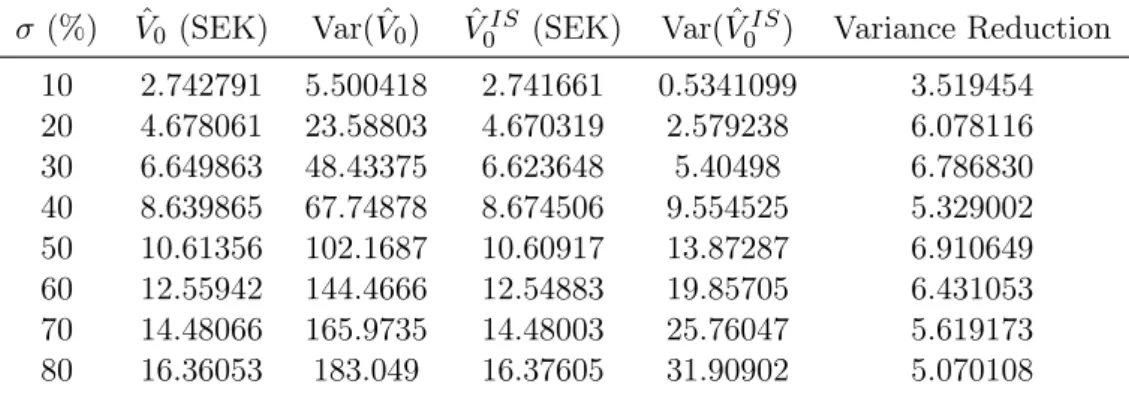
26 Table 5.2: Strike price K = 52 with 2nd-order polynomial
(%) ˆV0 (SEK) Var( ˆV0) Vˆ0IS (SEK) Var( ˆV0IS) Variance Reduction
10 2.742791 5.500418 2.741661 0.5341099 3.519454 20 4.678061 23.58803 4.670319 2.579238 6.078116 30 6.649863 48.43375 6.623648 5.40498 6.786830 40 8.639865 67.74878 8.674506 9.554525 5.329002 50 10.61356 102.1687 10.60917 13.87287 6.910649 60 12.55942 144.4666 12.54883 19.85705 6.431053 70 14.48066 165.9735 14.48003 25.76047 5.619173 80 16.36053 183.049 16.37605 31.90902 5.070108
Table 5.3: Strike price K = 54 with 2nd-order polynomial
(%) ˆV0 (SEK) Var( ˆV0) Vˆ0IS (SEK) Var( ˆV0IS) Variance Reduction
10 4.210878 3.812905 4.217694 3.041304 1.253707 20 5.936218 21.59282 5.971708 6.066479 3.559366 30 7.938367 53.66102 7.926904 9.451961 5.677237 40 9.86214 82.51658 9.870942 14.98291 5.507380 50 11.89708 110.3234 11.89167 19.19366 5.747908 60 13.81342 149.0316 13.81165 25.8025 5.775859 70 15.77979 202.9246 15.78673 36.79025 5.515717 80 17.64294 206.3911 17.65848 36.40016 5.670060
Table 5.4: Strike price K = 56 with 2nd-order polynomial
(%) ˆV0 (SEK) Var( ˆV0) Vˆ0IS (SEK) Var( ˆV0IS) Variance Reduction
10 6.004848 2.782589 6.008509 5.702775 6.557643 20 7.330201 25.71255 7.337774 7.855498 3.273192 30 9.219044 51.91792 9.218478 12.5676 4.131093 40 11.18193 83.24592 11.19667 16.43322 5.065710 50 13.17314 129.8683 13.18626 25.69518 5.054189 60 15.10658 141.4808 15.11283 15.11283 9.361635 70 17.07919 205.1197 17.07342 37.29034 5.500612 80 19.03812 202.4958 19.03074 43.91871 4.610696
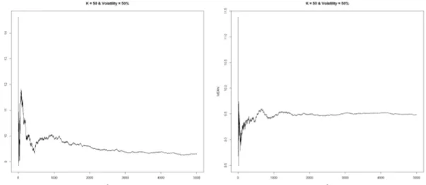
K = 50, r = 0.02, = 10% and T = 1. In figures 5.4 and 5.5 the same convergence behaviour is shown but with K = 54.
Figures5.6and5.7shows the same convergence behaviour of standard LSM and IS-LSM but this time with Hermite-polynomials. In figures 5.8 and 5.9 the same convergence behaviour is shown but with K = 54.
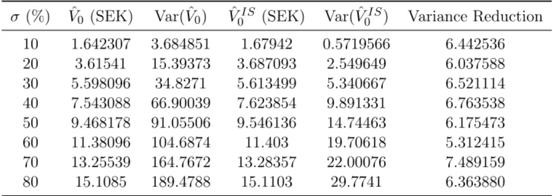
27 Table 5.5: Strike price K = 50 with Hermite-polynomials.
(%) ˆV0 (SEK) Var( ˆV0) Vˆ0IS (SEK) Var( ˆV0IS) Variance Reduction
10 1.642307 3.684851 1.67942 0.5719566 6.442536 20 3.61541 15.39373 3.687093 2.549649 6.037588 30 5.598096 34.8271 5.613499 5.340667 6.521114 40 7.543088 66.90039 7.623854 9.891331 6.763538 50 9.468178 91.05506 9.546136 14.74463 6.175473 60 11.38096 104.6874 11.403 19.70618 5.312415 70 13.25539 164.7672 13.28357 22.00076 7.489159 80 15.1085 189.4788 15.1103 29.7741 6.363880
Table 5.6: Strike price K = 52 with Hermite-polynomials. (%) Vˆ0 (SEK) Var( ˆV0) VˆIS
0 (SEK) Var( ˆV0IS) Variance Reduction
10 2.757571 6.208106 2.744517 2.744517 2.262003 20 4.729887 25.268483 4.711123 4.075598 6.199945 30 6.715419 35.679909 6.689882 7.853771 4.543029 40 8.686990 72.393169 8.685366 12.09995 5.982931 50 10.670997 110.528897 10.68087 17.51208 6.311580 60 12.584007 131.801013 12.56325 21.5633 6.112284 70 14.535953 153.505541 14.54229 30.16194 5.089379 80 16.392707 213.818094 16.42989 38.55391 5.545951
Table 5.7: Strike price K = 54 with Hermite-polynomials. (%) Vˆ0 (SEK) Var( ˆV0) VˆIS
0 (SEK) Var( ˆV0IS) Variance Reduction
10 4.228625 4.975201 4.210871 3.202642 1.553468 20 5.987346 28.069843 5.982083 5.187637 5.410911 30 7.911848 53.079082 7.899397 9.846293 5.390768 40 9.982095 74.236456 9.990763 14.10173 5.264351 50 11.927152 114.319966 11.94185 19.91554 5.740239 60 13.889657 155.462079 13.88364 23.89334 6.506503 70 15.828050 172.637771 15.80695 31.29834 5.515876 80 17.723791 228.226868 17.72223 38.06168 5.996237
Table 5.8: Strike price K = 56 with Hermite-polynomials. (%) Vˆ0 (SEK) Var( ˆV0) VˆIS
0 (SEK) Var( ˆV0IS) Variance Reduction
10 6.017468 1.189414 5.99501 6.266122 0.1898166 20 7.379858 35.090213 7.384168 7.872534 4.4572958 30 9.248224 68.370972 9.271849 12.81123 5.3368000 40 11.226492 87.284022 11.19545 17.65529 4.9437886 50 13.244236 134.337202 13.27871 25.90216 5.1863320 60 15.208831 166.926922 15.25854 35.36346 4.7203221 70 17.180185 206.949380 17.33694 35.91842 5.7616504 80 19.112274 227.486597 19.17055 45.69645 4.9782116
28
Figure 5.2: Convergence of put option using standard LSM (left) and IS-LSM (right) with 2nd-order polynomials and sample size of n = 5000. The pricing parameters here
are S0= 50, K = 50, r = 0.02, = 10% and T = 1.
Figure 5.3: Convergence of put option using standard LSM (left) and IS-LSM (right) with a sample size ofwith 2nd-order polynomials and sample size of n = 5000. The
29
Figure 5.4: Convergence of put option using standard LSM (left) and IS-LSM (right) with 2nd-order polynomials and sample size of n = 5000. The pricing parameters here
are S0= 50, K = 54, r = 0.02, = 10% and T = 1.
Figure 5.5: Convergence of put option using standard LSM (left) and IS-LSM (right) with 2nd-order polynomials and sample size of n = 5000. The pricing parameters here
30
Figure 5.6: Convergence of put option using standard LSM (left) and IS-LSM (right) with Hermite-polynomials and a sample size of n = 5000. The pricing parameters here
are S0= 50, K = 50, r = 0.02, = 10% and T = 1.
Figure 5.7: Convergence of put option using standard LSM (left) and IS-LSM (right) with Hermite-polynomials and a sample size of n = 5000. The pricing parameters here
31
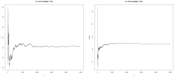
Figure 5.8: Convergence of put option using standard LSM (left) and IS-LSM (right) with Hermite-polynomials and a sample size of n = 5000. The pricing parameters here
are S0= 50, K = 54, r = 0.02, = 10% and T = 1.
Figure 5.9: Convergence of put option using standard LSM (left) and IS-LSM (right) with Hermite-polynomials and a sample size of n = 5000. The pricing parameters here
32
Results for optimal drift ✓
⇤The optimal ✓⇤ was found by running Algorithm3which estimates the IPA-Q estimator
of the second moment. By empirical methods, the starting values for the iterative scheme given by (4.16) was determined by looking at the reference ratio where the fraction is approximately equal to 1.
Figure5.10shows an the reference ratio V0IS-LSM
V0LSM for ✓ 2 [ 1.17, 1.15] with K = 56 and
= 50%. This interval corresponds to the reference ratio approximately to one for all ✓. Hence, an arbitrary starting value for ✓ is chosen between the interval [ 1.17, 1.15]. The sequence an in algorithm 4 is set according to the decreasing sequence n = 0.01n
for n = 1, ..., nMAX. For all simulations nmax = 10.000 and the threshold was set to
✏ = 10 7.
Figure 5.10: Reference ratio vs ✓ 2 [ 1.17, 1.15] with K = 56 and = 50%.
Tables5.9 and5.10 shows the optimal values for ✓⇤ for both 2nd-order polynomials and
33
Table 5.9: Optimal ✓ using second order polyomials. (%) K = 50✓⇤ K = 52✓⇤ K = 54✓⇤ K = 56✓⇤ 10 1.61 1.33 1.09 0.86 20 1.49 1.38 1.25 1.16 30 1.43 1.35 1.28 1.2 40 1.34 1.29 1.25 1.2 50 1.31 1.28 1.22 1.16 60 1.25 1.21 1.17 1.15 70 1.19 1.16 1.11 1.1 80 1.13 1.1 0.94 1.06
Table 5.10: Optimal ✓ using using Hermite-polynomials. (%) K = 50✓⇤ K = 52✓⇤ K = 54✓⇤ K = 56✓⇤ 10 1.59 1.33 1.09 0.83 20 1.49 1.37 1.28 1.16 30 1.43 1.34 1.27 1.2 40 1.35 1.3 1.25 1.2 50 1.28 1.25 1.21 1.16 60 1.24 1.22 1.18 1.11 70 1.21 1.15 1.15 1.1 80 1.15 1.1 1.1 1.06
Chapter 6
Discussion
This thesis presents a variance reduction method for pricing American options using GBM. The LSM method is studied using two different but yet fundamental basis func-tions for the backward iterative least-square regression step. By implementing the impor-tance sampling procedure in the LSM method resulting as IS-LSM method, the reduction of variance compared to standard LSM-method is well noticable.
Comparing the usage of second order polynomials with Hermite-polynomial did not give any significant difference in the price. In this thesis, the underlying asset is a simple one-dimensional GBM, meaning that the difference in price estimation between these two choices of basis functions is not very remarkable. As Longstaff & Schwartz uses more complex instruments in their original paper such as pricing interest rate swaps, the choice of "good" basis functions gets more critical for estimating the continuation value, without adding bias to the pricing step. When looking at the variance for different strike prices and different volatilities, it is clear that the dominating factor for higher variance is a higher volatility. The value of for which the variance of the put price estimator gets very high is between 2 [70%, 80%] for both second order polynomials and Hermite-polynomials.
When simulating the drifted GBM, the choice of a good reference price of the option in terms of the reference ratio is indeed a good method for knowing that the option is priced correctly. A challenge however was the large amount of time consumption in finding the reference ratio for which the fraction is very close to 1. Figure 5.10 shows clearly that it is difficult to choose the right ✓ corresponding to the "correct" ratio V0IS-LSM
V0LSM ⇡ 1. In
fact, this was computationally challenging since pricing had to be done several times over different values for ✓. When running Algorithm 3 there was a deviation for which the sequence ✓n+1 = ✓n ngn(✓n) converged to ✓⇤. For some runs, ✓⇤ deviated very much
from the empirical ✓⇤ for which the starting value was chosen. The reason for this may
35 rely on the fact that each simulated scenario is dependent on the optimal stopping time ⌧⇤, and cashflows in time 0 t T can be very different depending on ⌧⇤.
Nevertheless, the difficulty in finding ✓⇤, the estimated price after running IS-LSM gave
a much lesser variance in comparison to LSM. At most, the reduction of variance was up to the factor of 9 time less than the original LSM. But for most cases, the reduction was around 5 times less compared to standard LSM. Both tables 5.9 and 5.10indicate that for a larger and K, the smaller the value of the drift ✓ is needed. As S0 = 50, for strike
price K = 50, the value of ✓ over higher gets a significant decrease in comparison to cases with K = 52, ..., 56.
The results presented by Moreni paper are not comparable in the sense that he uses con-stant volatility when pricing over different strike prices. Moreover the choice of interest rate is different and the models are multidimensional. However, for higher K the drift ✓ gets smaller similarly to tables5.9and 5.10.
The way of implementing a good pricing engine is relevant. For this thesis all the implementation was written in R which is optimized for vector calculation and is not very efficient in handling <for> loops. Since some parts of the LSM-algorithm requires using <for> loops, the total pricing engine for finding the optimal drift ✓ increased the computational time dramatically which limited the efficiency of both time saving and CPU usage. For this reason a high-level programming language is recommended. Even if in this thesis there is no comparison presented for the choice of discretization method for scenario generation, the usage of Millstein-1 scheme compared to Euler-Maryama during test-simuluations was slower. This is due to the extra term given in (3.6). This should have been considered since Euler-Maryama scheme would most likely be equivalent but more efficient.
Important sampling is an efficient method for reducing variance of an estimator. This thesis presented the change of drift in the underlying GBM by means of the Girsanov theorem. The pricing of American put option on a stock price using IS-LSM is efficient. However, this method may even be a better alternative for more complex instruments with early exercise opportunity rather than a single stock based on GBM.
Appendix A
Essential supernum
This explanation is taken from a short course in optimal stopping problem by Damien Lamberton in [8], where the details about the Snell envelope is also well explained. Here we only take into account the essential supernum which occurs in equation (2.7). It is well known that if (Xn)n2Nis a sequence of real valued random variables, supn2NXn
is a random variable (with values in R [ {+1}). When uncountable families of random variables have to be considered, as occurs in the theory of optimal stopping, the notion of essential upper bound is needed.
Theorem A.1. Let (Xi)i2I be a family of real valued random variables (with a possibly
uncountable index set I). There exists a random variable ¯X with values in ¯R, which is unique up to null events, such that
1. For all i 2 I, Xi X a.s.
2. If X is a random variable with values in ¯R satisfying Xi X a.s., for all i 2 I,
then ¯X X a.s.
Moreover, there is a countable subset J of I such that ¯X = supi2JXi a.s.
The random variable ¯X is called the essential upper bound (or essential supremum) of the family (Xi)i2I and is denoted by ess supi2IXi.
Proof. By using a one-to-one increasing mapping from ¯R onto [0, 1], we can assume that the Xi’s take on values in [0, 1]. Now, given a countable subset J of I, set
¯
XJ = sup i2J
Xi.
37 This defines, for each J, a random variable with values in [0, 1]. Denote by P0 the set of
all countable subsets of I and let:
↵ = sup
J2P0
E ¯XJ.
Consider a sequence (Jn)n2N of elements in P0 such that limn!1E ¯XJn = ↵. The union
J⇤ =Sn2NJn is a countable subset of I and we have ↵ = E ¯XJ⇤. It can now be proved
that the random variable ¯X = ¯XJ⇤ satisfies the required conditions. First fix i 2 I.
The set J⇤ [ {i} is a countable subset of I and ¯X
J⇤[{i} = max( ¯X, Xi). Therefore,
E max( ¯X, Xi) E ¯X and max( ¯X, Xi) = ¯X a.s., which means that Xi ¯X a.s.. Now
consider a random variable X such that X Xi for all i 2 I. Since J⇤ is countable, we
Bibliography
[1] S. Asmussen and W. Glynn. Stochastic Simulation, Algorithms and Analysis, vol-ume 57. Springer, 2009.
[2] G. Cesari, J. Aquilina, N. Charpillion, Z. Filipov`c, G. Lee, and I. Manda. Modelling, Pricing and Hedgning Counterpary Credit Risk, volume 1. Springer, 2009.
[3] E. Clèment, D. Lamberton, and P. Protter. An analysis of a least squares regression method for american option pricing. In Finance and Stochastics 6, 449-471, 2002. [4] J.C. Cox, S.A. Ross, and M Rubinstein. Option pricing: A simplified approach. In
Journal of Financial Economics, 1979.
[5] H. Föllmer and A. Schied. Stochastic finance: an introduction in discrete time (2 ed.), volume 2. Walter de Gruyter, 2004.
[6] P. Glasserman. Monte Carlo Methods in Financial Engineering, volume 53. Springer, 2003.
[7] C. Graham and D. Talay. Stochastic Simulation and Monte Carlo Methods, vol-ume 68. Springer, 2003.
[8] D. Lamberton. Optimal stopping and american options. Universitè Paris-Est, 1(1):3–4, September 2002.
[9] F.A. Longstaff and E.S. Schwartz. Valuing american options by simulation: A simple least square approach. In The Review of Financial Studies, 2001.
[10] N. Moreni. Pricing american options: A variance reduction technique for the longstaff-schwartz algorithm. Review of Scientific Instruments, 72(12):4477–4479, December 2003.
[11] Y. Su and M. Fu. Optimal importance sampling in securities pricing. Journal of Computational Finance, 5(4):27–50, December 2002.
TRITA -MAT-E 2016:64 ISRN -KTH/MAT/E--16/64-SE