Can money be made on Mondays? : An empirical investigation of the efficiency on the OMXS30

J

I

B

S

JÖNKÖPING UNIVERSITY

C a n m o n e y b e m a d e o n M o n d a y s ?

An empirical investigation of the efficiency on the OMXS30

Master thesis within Finance

Author: Catrin Jakobsson Ola Henriksson

Tutor: Daniel Wiberg

Master’s Thesis in Finance

Title: Can money be made on Mondays? – An empirical investigation of the efficiency on the OMXS30

Author: Catrin Jakobsson, Ola Henriksson Tutor: Daniel Wiberg, Andreas Högberg

Date: 2010-05-24

Subject terms: Efficiency, Efficient market theory, Anomaly, Monday effect, Weekend effect, January effect, Day-of-the-week effect, Turn-of-the-year effect, Abnormal returns

Abstract

Purpose: The purpose of this thesis is to investigate if abnor-mal patterns concerning the rates of return during specific weekdays and months are observable for the companies in the OMXS30 during the period 2003-2010. A special focus will be put on the Monday ef-fect anomaly.

Background: Investors have a tendency to search for investment opportunities. If errors exist in the pricing of stocks it indicates that anomalies are present and that the stock market is inefficient. Investors then have the possibility to utilize the anomalies in order to re-ceive above average returns.

Method: This study is using data of stock prices from Nasdaq OMX in the period of 2003-2010. The strength and existence of the Swedish stock market efficiency is measured through autocorrelation-, chi-square- and regression tests. Average monthly stock returns are calculated on daily-, monthly-, and yearly basis. The returns are compared in order to examine if day-of-the-week and turn-of-the-year anomalies exist.

Conclusion: No Monday effect is found in 2003-2010. However, positive Thursday- and positive Friday effects are detected. A negative turn-of-the-year effect as well as a positive April effect is found. The investment opportunities that could be utilized in 2003-2010 due to the specific anomalies in the period do not

necessarily imply that the same anomalies can be expected on the OMXS30 in the future.

Table of Contents

1

Introduction ... 1

2

Theoretical Background ... 2

2.1 Efficient Market Theory and its flaws ... 2

2.2 Description of different anomalies ... 3

3

Review of studies regarding stock market patterns ... 4

3.1 Investigations of autocorrelation between stock returns ... 4

3.2 Investigations of the day-of-the-week effect ... 4

3.3 Investigations of the turn-of-the-year effect ... 6

3.4 Summary of main empirical findings ... 8

4

Methodology and Data ... 9

4.1 How stock returns are calculated ... 9

4.2 Dependency between stock returns ... 10

4.3 Test of the day-of-the-week effect... 11

4.4 Chi-square test of the Monday effect ... 11

4.5 Test of the turn-of-the-year effect ... 11

5

Empirical Findings and Analysis ... 12

5.1 Evidence of market efficiency using autocorrelation ... 12

5.2 Weekday returns indicate market inefficiency ... 13

5.3 The non-existing Monday effect ... 14

5.4 An unexpected turn-of-the-year effect ... 14

6

Conclusion ... 17

List of references ... 18

Table 3.1 ... 19

1

Introduction

The Efficient Market Theory (EMT) was first introduced by Fama (1965), and accord-ing to him an efficient market is a market where the stock prices at every point in time give a correct estimate of the intrinsic value. However, empirical investigations have found evidence of stock price anomalies. This means that patterns of unpredictable rates of return, according to the theory of efficient market, have been observed.

An anomaly is a deviation of what is claimed by theory and implies that the stock mar-ket is not efficient. Explanations for why anomalies exist have still not been found (Claesson, 1987). An example of an anomaly is the day-of-the-week effect, which more specifically can be a Monday effect. Cross (1973) and French (1980) explain the Mon-day effect in the following way: “average returns on MonMon-days are lower than for any other day of the week”. The day-of-the-week effect is however not specific for only Mondays, but can occur on any weekday. Another well-known anomaly is the turn-of-the-year effect, which implies abnormally high positive stock returns during January (Ritter, 1988).

If there exists an anomaly on the Swedish stock market, which means that the EMT does not hold, it indicates that the market is inefficient.This will result in investors hav-ing the possibility to receive higher returns on their investments until widespread awareness of the pattern arises and the anomaly automatically disappears. An inefficient market constitutes a problem for those investors who do not possess the knowledge of an existing anomaly, since they will risk investing on the wrong occasion and thereby receive lower returns on their investments.

The purpose of this thesis is to investigate if abnormal patterns concerning the rates of return during specific weekdays and months are observable for the companies in the OMXS30 during the period 2003-2010. A special focus will be put on the Monday ef-fect anomaly.

Compared to studies made on other stock markets, few investigations have been done on the Swedish stock market. Studies have mainly covered the U.S. market. Given the lack of studies made on the Swedish market and especially during the last decade, it is interesting to see if day-of-the-week and turn-of-the-year effects exist on the Swedish stock market in 2003-2010.

Economists find it hard to explain the causes of the anomalies. Damodaran (1989) tries to explain the Monday effect in that firms tend to announce bad news on Fridays, which is reflected in the stock price of the upcoming Monday. This explanation has also been suggested by several others. However, Damodaran finds that the Monday effect could only be influenced by announcements of bad news on Fridays up to approximately 3,4 percent.

The remainder of the thesis is structured as follows:

Section 2 describes the efficient market theory and the anomalies; day-of-the-week ef-fect, the Monday efef-fect, and the turn-of-the-year effect. Section 3 reviews previous em-pirical investigations that concerns stock market efficiency on the Swedish stock market and other stock markets. Section 4 presents information of how the empirical

investiga-and discusses the results from the empirical investigation. Section 6 concludes the the-sis.

2

Theoretical Background

The following sections present the efficient market theory and the most common anomalies as of today.

2.1 Efficient Market Theory and its flaws

Stock market efficiency implies that an investor is not able to earn above average re-turns on investments unless the investor takes on additional risk (Malkiel, 2003). Fama (1970) describes the EMT as efficientif it fulfils three different conditions. Firstly, trad-ing in securities is not attached with transaction costs. Secondly, all information is available to all of the investors. Thirdly, all of the investors agree that the price of the security reflects the information available. Though, the EMT does not necessarily have to fulfil all of the three conditions on a constant basis. Even if Fama’s three sufficient conditions for EMT advocate that all information is available, the price of a security does not always have to be right and correspond to the intrinsic value. The movement in the stock price should reflect the knowledge and expectations by all the investors.

Fama (1970) also describes that there exist three different levels when it comes to effi-ciency, namely a strong-, a semi-strong-, and a weak level. The weak level of efficiency indicates that the stock price is decided by past stock prices, and follows a so-called random walk pattern. Calculation of future stock prices with a technical analysis ap-proach is impossible. Semi-strong efficiency includes public information in addition to the information in the level of weak efficiency. For example, when a company an-nounces news that affect the stock price, the stock will be traded accordingly since the change is reflected in the price instantly. The strong efficiency form includes all the in-formation as for the weak- and semi-strong efficiency, as well as insider inin-formation. In a strong efficient market it is impossible for any investor to make above average return on stocks, not even for investors with inside information, since all the information is al-ready included in the stock price.

Malkiel (2003) explains that future stock prices can partially be predictable over short time intervals by irrational investors. Thus the market cannot be perfectly efficient, only efficient depending on the amount of information that is revealed in the market and how the information is utilized by investors. Ritholtz (2004) believes the EMT is outdated, due to the fact that stock prices are not random or unpredictable. Ritholtz continue to explain that according to the EMT an investor cannot outperform the market. As a con-tradiction studies have shown that a stock’s value outperforms a stock’s growth, which is a situation that cannot occur in a truly efficient market. Another error with the EMT according to Ritholtz is the possibility for market crashes, bubbles, and irrational price swings. In an efficient market, these phenomena should not exist if prices are reflecting all known information about the stock.

2.2 Description of different anomalies

An anomaly is a registered pattern that contradicts the EMT (Cross, 1973; French, 1980). If an anomaly is found it gives investors the possibility to, potentially, create trading strategies that are beneficial so that they can take advantage of the anomaly. Though if transactions costs and risk premiums are too high, it will reduce the above average returns the investors make on the strategies, and an anomaly which at first would indicate an inefficient market is instead a part of an efficient market (Kohers, Kohers, Pandey, and Kohers, 2004). Examples of anomalies are the so-called Monday effect, day-of-the-week effect, and the size effect. Keim (1983) explained the “size ef-fect” on the market as an effect where it is easier to get higher returns by investing in small-sized companies compared to large-sized companies. According to Claesson (1987), the size effect can be explained by the higher risk associated with small-sized companies and the investor should therefore be compensated with higher returns. An-other anomaly is the “seasonal effect” where market returns fluctuate during the seasons of the year. One of the most famous seasonal effects is the turn-of-the-year effect, where the stock market has a tendency to have higher returns in January than during the other months of the year.

The EMT suggests that stock returns should be of the same size no matter what day of the week it is. Studies have shown that the return on some of the weekdays is lower or even negative compared to other days of the week (Gibbons & Hess, 1981). If returns on Mondays are lower than for other weekdays the result is a Monday effect, which is a typical day-of-the-week anomaly. Even though tests have been executed trying to reveal the reason for why a day-of-the-week anomaly would exist, the results have been insuf-ficient or even considered as miscalculations according to Albertsson, Eriksson, and Lundberg (2005). However, Sias and Starks (1995) give some explanations for why a Monday effect can exist. Investors have a tendency to trade less during Mondays, which in turn causes returns to be lower than for other days. Also, stock brokers usually issue recommendations to buy during the beginning of the week and then later during the week they recommend investors to sell.

Ritter (1988) explains the turn-of-the-year effect as stocks having abnormally high re-turns during the last trading days of December and through January. This anomaly has been registered regularly and with significant magnitude during the years 1971-1985. The turn-of-the-year effect is referred to an anomaly due to the lack of provided expla-nations for its existence. However, Griffiths and Winters (2005) propose two often used explanations for why the anomaly is present. The first one is the tax-loss hypothesis which states that investors sell their shares before the end of the year and re-purchase them during January. Investors do this in order to reduce the payable taxes made from shares that have brought profit over the year, presupposing that tax costs are paid re-troactive. The second explanation is the risk-shifting window dressing hypothesis which describes the correlation between supply and demand for shares and securities during the month of December. Fund managers tend to switch from risky- and high return se-curities to less risky- and lower return sese-curities and thereby realizing the profits that have been earned during the year.

3

Review of studies regarding stock market patterns

Previous empirical investigations concerning stock market efficiency and anomalies on global stock markets are presented in the following sections. The final section is a summary of the main investigations within the subject.

3.1 Investigations of autocorrelation between stock returns

Claesson (1987) investigates the autocorrelation of two following day’s stock returns for 49 Swedish stocks in the time period 1978-1984. The daily returns used are of the type category one used in this study. The regression results in a beta value of 0,0081 which indicates a weak linear relationship between stock returns. The R-square value from the investigation shows that only 0,9 percent of the current day’s stock return is explained by the previous day’s return. Both these values are signs of an efficient Swe-dish stock market during 1978-1984.

Fama (1965), Jennergren and Korsvold (1973) examine the American- versus Norwe-gian and Swedish stock markets for autocorrelation between stock returns. They discov-er that the previous day’s stock return affect the current day’s stock return with 0,3 pdiscov-er- per-cent in the U.S. market in the period 1957-1962. The corresponding value for the Nor-wegian and Swedish market in 1967-1971 is 1,4 percent. These values indicate efficien-cy on the three stock markets respectively during their specific time periods.

3.2 Investigations of the day-of-the-week effect

Wang, Li, and Erickson (1997) search for and find a pattern of a day-of-the-week effect on the U.S. stock market, namely a negative Monday effect, during 1962-1993. They investigate three different indexes. Sun and Tong (2002) continue in the direction that is laid out by Wang, Li, and Erickson, and carry out a similar investigation for the period 1962-1998. They come across a negative Monday effect as well; however it is mainly observable in the last week of each month. In the third week they instead detect a nega-tive Friday effect, and therefore suggest that there may exist a week-four effect. Overall, the returns during the fourth week are the lowest of the month, but are especially low for the Monday in that week.

Many investigations have observed that weekdays other than Mondays are attached with significantly lower rates of returns than the average. For example, Davidsson (2006) in-vestigates the U.S. stock market by looking at the S & P 500 index in 1970-2005, and observes that returns on Wednesdays are much lower than for any other day of the week. He also finds evidence of a negative Monday-effect and a weekend-effect, how-ever the average Wednesday return is much more abnormal.

Claesson (1987) carries out an investigation of the weekdays on the Swedish stock mar-ket during 1978 – 1984, and discovers that the average returns are of different sizes. The findings are shown in table 3.1. Claesson notices that Monday and Friday have the highest average returns, and that Tuesday has the lowest average return. Among the weekdays, the return on Tuesdays deviate the greatest from the average weekday return of 0,131 percent, with a deviating value of 0,158 percent. The corresponding deviation from the average weekday return for Mondays and Fridays are smaller, with values of

0,063 and 0,118 percent respectively. To conclude, the data shows a negative Tuesday effect on the Swedish stock market in 1978-1984.

Table 3.1 Claesson’s finding of the day-of-the-week effect in Sweden 1978-1984.

Monday Tuesday Wednesday Thursday Friday All days Average return

(percent) 0,194 -0,027 0,112 0,139 0,249 0,131 Std dev 1,997 1,917 1,876 1,835 1,775 1,883 Observations 13 716 14 894 15 341 15 045 14 373 73 369

The negative Tuesday effect in Claesson’s study is even more evident when looking at the average weekday returns for each of the companies separately. The lowest return occurs on Tuesdays for 34 companies out of the total number of 49. This can be com-pared with that only two companies have their most negative returns on Mondays. In terms of the average Friday return, 23 out of 49 stocks are being positive, thereby mak-ing Friday the weekday with the greatest return in the sample.

The procedure undertaken in Claesson’s study is also carried out by another study in Sweden. Albertsson et al (2005) investigate the period 1996-2004, and they find no strong evidence of a day-of-the-week effect. Out of nine investigated indexes, represent-ing the stock market’s different industries, only two of them support the Monday effect, and it is only observable to a weak extent in the period 1996-1999.

Several empirical investigations regarding the day-of-the-week effect examine the U.S. stock market, and they are presented in the following three paragraphs. They observe trends of negative returns on Mondays, and highly positive returns on Wednesdays. These findings are different to what Claesson finds on the Swedish market during the period 1978-1984.

French (1980) examines the S & P in the period 1953-1977 and detects an average Monday return of -0,1681 percent which is abnormally lower than the other weekday returns. French therefore concludes that the U.S. stock market is inefficient. However, creating a trading strategy based on the knowledge of negative returns on Mondays will not be profitable according to French due to the transaction costs that have to be taken into account. Such a trading strategy will not be of economic significance and the anomaly can as a result not be utilized. Two other findings by French, that further strengthens an observed inefficient market, are positive Wednesday- and positive Fri-day effects. They have abnormally high returns of 0,0967 and 0,0873 percent. In order to grasp how much these weekday returns deviate from what is expected during the pe-riod, an average weekday return of 0,01528 is used as a comparison.

Gibbons and Hess (1981) look at the S & P 500 index in 1962-1978 and also find that weekdays’ stock returns in the U.S. are of different sizes. The Monday return is the only negative among the weekday returns, with a value of -0,134 percent. The Monday return is abnormal compared to the other weekdays so it is reasonable to assume that a nega-tive Monday effect exists. Wednesdays’ and Fridays’ average stock returns of 0,096 and 0,084 percent are higher than the average weekday return of 0,0152 percent, thus indi-cating positive Wednesday and Friday effects in 1962-1978.

Keim & Stambaugh (1984) also investigate the S & P 500 index but extends the time period to 1953-1982. They find that there exists a negative Monday effect where returns on Mondays’ are abnormally low with a value of -0,1539 percent. Their result as well show abnormal positive returns during Wednesdays and Fridays of 0,1028 and 0,092 percent. Comparing the weekday returns with the average return for the whole week of 0,02062 percent the effects mentioned are evident.

Kohers et al (2004) investigate the 12 largest stock markets in the world during the 80´s and 90´s in order to detect if improvements in market efficiency have caused the day-of-the-week effect to disappear. They find that the anomaly is evident during the 80´s and has decreased in the 90´s and almost disappeared. They also discover that the day-of-the-week effect, e.g. in Japan and Australia, is most apparent during Tuesdays. Kohers et al (2004) explain that the market efficiency has improved over time which in turn has caused the day-of-the-week effect to disappear.

3.3 Investigations of the turn-of-the-year effect

Keim (1983) searches for a turn-of-the-year effect in the period of 1963-1979 for NYSE Amex. He finds evidence of the anomaly and discovers that the size dimension of it is increasing throughout the specified period. The anomaly is significantly apparent during the first five days of January. The investigation also observes a negative relation be-tween the turn-of-the-year effect and the size effect.

Haug and Hirschey (2006) test both large-cap and small-cap in the U.S. and investigate a sample of 202 years. They want to test if the Tax Reform Act1 of 1986 has affected the stock market in terms of anomalies and the window dressing theory discussed by Griffiths and Winters (2005). They find that the turn-of-the-year effect does not exist in large-cap markets. Abnormally high rates of returns in January are however found in the cap markets. This finding, according to Haug and Hirschey, means that the small-cap market has been unaffected by the Tax Reform Act. Thus, the hypothesis of win-dow dressing is not rejected when it comes to the small-cap market. Their result shows that the hypothesis may have contributed to the January effect after the Tax Reform Act was implemented.

Claesson (1987) clarifies that the most often used argument trying to explain the exis-tence of turn-of-the-year effect is the tax-loss hypothesis. If investors however are aware of a positive January effect, the question remains unanswered regardingwhy they do not sell their stocks a few weeks earlier and reinvest their money in stocks during December. Claesson explains that investors may do this in order to benefit from the January effect and make greater profits. Though, Claesson makes it clear that even though an investor can potentially make money in the month of January by investing during December, the investor cannot be certain that the specific stock will generate a positive payoff in January. She continues by pointing out that it is not certain that the month of January is attached with positive stock returns in the future. Claesson further presents two reasons for why the tax-loss hypothesis cannot be the only explanation of the turn-of-the-year effect’s existence. First of all, there are a lot of objections against

1 _{1986, President Ronald Regan (USA) signs the Tax Reform Act, the legislation simplifies the process of} paying taxesfor millions of Americans and makes rid of loopholes.

the underlying theory of the hypothesis. Secondly, some countries do not have the poli-cy with retroactive tax cost, e.g. Japan and Canada, but still the turn-of-the-year effect is found. Furthermore, Claesson explains two reasons for why the theory of turn-of-the-year effect can hold. Most studies show that the return in January can be explained, to some extent, by the tax-loss hypothesis.Additionally, the effect has not been found be-fore the tax reform act was introduced in the U.S.

Two studies investigate the turn-of-the-year effect on the Swedish stock market, and they examine two different time periods. The first one concerns 1959-1979 and finds abnormally high average returns in January and July (Gultekin & Gultekin, 1983). The respective monthly returns are 4,00, and 2,41 percent. When looking at monthly returns that are abnormally low, two such values are noticeable. September has the lowest value of -1,34 percent, and August has a value of -1,10 percent. The second study takes a look at the time period 1978-1985. Claesson (1987) finds three months with abnormally high average returns. Two of them are the same as for the previous period, namely January and July. In addition, the month of November has abnormally high returns. Their re-spective values are 8,73, 4,88, and 5,46 percent. All of these monthly returns are greater than the positive abnormal returns in the previous time period study. Only one month in this time period on the Swedish stock market has an average return that is abnormally low, namely September. However, the September monthly return of -1,48 percent is not very different to the negative September return in the period 1959-1979 of -1,34 cent. In 1959-1979 the average monthly return over the years is approximately 0,60 per-cent, whilst for the period 1978-1985 it is 2,52 percent. Two noticeable and interesting movements of the monthly returns between the two time periods are the ones in January and November. Both of their monthly returns have increased a great extent between 1959-1979 and 1978-1985. They moved from 4,00 to 8,73 percent in January, and from -0,18 to 5,46 percent in November.

The turn-of-the-year effect is also examined on the U.S. stock market. The study by Givoly and Ovadia (1983) investigate two time periods; 1945-1979 and 1975-1979. The monthly returns in the periods follow the pattern recognized on the Swedish stock mar-ket, namely that in short time periods they are more abnormal and of greater values than in longer periods. In 1945-1979, three months are observed with abnormally high aver-age returns. January, November, and December have monthly returns of 4,36, 2,24, and 2,17 percent. No month in the period is found with an abnormally low return. For the shorter time period, 1975-1979, four months have higher monthly returns than average. January constitute the month with the greatest return, a value of 10,20 percent. March, June, and November have monthly returns of 4,66, 4,70, and 5,12 percent. The month of October is the only month found in the short time period with an abnormally low return, a value of -5,44 percent.

When comparing the studies made on the Swedish and U.S. stock market, positive January effects are recognized. Two other mutual trends are observed. November is the month that has had positive abnormal returns during the majority of the investigated years, Another similarity between the stock markets is that the monthly return during September constantly has negative returns.

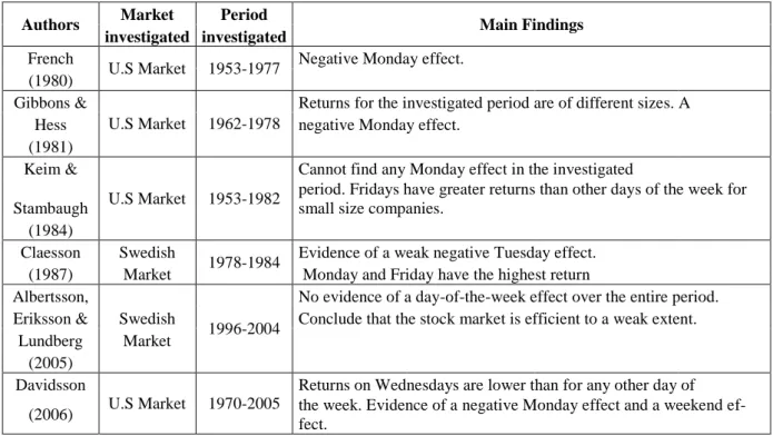
3.4 Summary of main empirical findings

Some previous studies investigating the day-of-the-week anomaly are summarized in table 3.2. The studies show findings of Monday-effects and other weekday-effects, while at the same time some of them do not find any anomalies. Investigations of the Swedish stock market have not found evidence of a Monday effect so far.

Table 3.2 Main findings from investigations of the day-of-the-week effect.

Authors Market Period Main Findings

investigated investigated

French

U.S Market 1953-1977 Negative Monday effect.

(1980)

Gibbons &

U.S Market 1962-1978

Returns for the investigated period are of different sizes. A

Hess negative Monday effect.

(1981)

Keim &

U.S Market 1953-1982

Cannot find any Monday effect in the investigated Stambaugh

period. Fridays have greater returns than other days of the week for small size companies.

(1984)

Claesson Swedish

1978-1984 Evidence of a weak negative Tuesday effect.

(1987) Market Monday and Friday have the highest return

Albertsson,

1996-2004

No evidence of a day-of-the-week effect over the entire period. Eriksson & Swedish Conclude that the stock market is efficient to a weak extent.

Lundberg Market

(2005)

Davidsson

U.S Market 1970-2005

Returns on Wednesdays are lower than for any other day of

(2006) the week. Evidence of a negative Monday effect and a weekend

ef-fect.

In table 3.3 the findings from a number of studies investigating the turn-of-the-year ef-fect are presented. The January efef-fect is found in all of them. Also some negative monthly effects are observed in the studies.

Table 3.3 Main findings from investigations of the turn-of-the-year effect.

Authors Market Period Main Findings

investigated investigated

Keim

U.S Market 1963-1979 Evidence of the anomaly throughout the investigated period,

(1983) especially during the first five days of January.

Givoly &

U.S Market 1945-1979

Returns during January are the greatest during the investigated

Ovadia period. Negative returns during June and September

(1983)

Givoly &

U.S Market 1975-1979

Abnormally high returns in January. Negative returns in September

Ovadia and October.

(1983)

Gultenking & Swedish Evidence of turn-of-the-year effect in January where returns are Gultenking Market 1959-1979 abnormally high. Negative returns in six out of twelve months.

(1983)

Claesson Swedish

1978-1985 Strong evidence of a positive January effect. The month of

(1987) Market September has the lowest return in the time period.

Haug &

U.S Market 1802-2004

A positive January effect in small cap markets. No evidence of any

4

Methodology and Data

The purpose of the thesis is to investigate if the day-of-the-week and the turn-of-the-year effect exist among the current 30 most traded Swedish companies that are included on the OMXS30 index in 2003-2010.

The OMXS30 index is a market-weighted index and contains the 30 companies that have the highest turnover on the Nordic stock market in Stockholm. The specific com-panies included in the index are revised twice a year, in January and in July. The current composition of the index is found in appendix 1. The index has a base value of 125 in 30th September 1986 (OMXS Local Index, 2010). This particular index is chosen since it represents the most frequently traded stocks in Sweden. Due to the high liquidity of the stocks, an ordinary investor is able to utilize the information that is found in this in-vestigation.

Data of each trading day’s last return is collected from the website Nasdaq OMX. In ad-dition, sizes of dividends paid out with its respective dates, splits, bonus issues, new is-sues, and special offers to the stockowners are considered and reflected in the data. This information is available on the website of Nasdaq OXM and in the companies’ respec-tive annual reports.

The investigation replicates the methods used in the study done by Claesson (1987). The method is based on collected data for the investigated period and calculations on market efficiency are carried out. The weak form of the efficient market theory is tested by autocorrelation. The semi-strong form of efficiency is tested by examining the day-of-the-week effect and the turn-of-the-year effect. The Monday effect is specifically tested with a chi-square test.

4.1 How stock returns are calculated

Two separate categories of returns are computed. The first category of returns is calcu-lated considering stock prices of all trading days. The second category only calculates returns that consider stock prices of trading dates that directly follow each other. Re-turns of trading days that have a non-trading-day in between are therefore excluded. Other dates that are further lifted from of the data set are those when dividends are paid out and when issues and splits are carried out. However, returns between Fridays and Mondays are still included.

The daily stock return of a stock from one day to another, i.e. the first category of re-turns, will be adjusted to reflect dividends, issues, and splits. The returns are turned into the second category of returns in the following way. If the stock has been registered without the dividend, the whole amount of the dividend is added to the current day, when calculating the return between the previous and the current day. After an issue and a split, the current day’s stock price is recalculated in order to be comparable with the stock price of the previous day. For example; a split of 5:1 results in the stock price be-ing multiplied by 0.75. A new issue is adjusted to reflect the difference between the previous day’s stock price and the subscription price. If the new issue is e.g. 1:5 à 100 SEK, the stock price of the previous day is subtracted by 100 SEK. The remaining stock price is then divided by 6 in this specific example. If the issue is 1:4, the price will be

price is then comparable to the previous day’s real stock price and the return between the two days can be calculated.

The adjusted stock prices of the two categories are used to calculate the returns between two following days with transactions over the seven-year period for each of the 30 stocks. The returns are calculated both in terms of percental- and logarithmic returns ac-cording to equations [1] and [2].

Percental daily return: rt = ((pt – pt-1) + d) / pt-1 [1] The current day’s stock price is denoted by pt, and the previous day’s stock price is de-noted by pt-1. If a potential dividend is paid out during the current day, the value of it, d, is added to the numerator.

Logarithmic daily return: r´t = ln((pt + d) / pt-1) [2] The average return of the each month is the sum of the daily returns during the month, displayed in equations [3] and [4].

Percental monthly return: (1+Rm) = (1+r1) x (1+r2) x ... x (1+rt) [3] Logarithmic monthly return: ln(1+Rm) = ln(1+r1) + ln(1+r2) + ... + ln(1+rt) [4] The relationship between the percental and logarithmic return is demonstrated in equa-tion [5].

(1+rt) = e^(r´t) [5]

The average yearly returns of the companies and as a total are calculated as the sum of the monthly returns divided by the number of observations.

4.2 Dependency between stock returns

The reason why autocorrelation is examined is to reveal if there exists a potential linear dependency between returns from one day to another. If the investigation finds a depen-dency between returns, it indicates that the stock market is not efficient in the weak form. The null- and alternative hypothesis are presented in equation [6]. The null hypo-thesis predicts that the stock market is efficient with no linear relationship between two following days’ stock prices.

H0 : β = 0 [6]

HA : β ≠ 0

The linear regression model in equation [7] is used.

rt+1 = β rt + error [7]

The coefficient β is estimated from the time-series of returns and received by the soft-ware program SPSS. The value of it can range from minus one to plus one. According to an efficient market the value of β should be close to zero.

The returns used in the autocorrelation model are logarithmic, and computed according to the first category of returns; i.e. returns are calculated between dates of trading,

ig-An average autocorrelation coefficient for the 30 companies is calculated in order to find out the average coefficient of determination, R2, for the index. The calculation pro-cedure is presented in equation [8]. The coefficient reveals how much of each daily stock return that is caused by the return of the previous trading day.

R2 = (∑i=30 βi2) / 30 [8]

4.3 Test of the day-of-the-week effect

Returns of the second type of category are used for the calculation of the average week-day returns. The average return is computed for the 30 stocks as a total and for each weekday separately, during the whole period 2003-2010. The same computation is also done for each year individually. In order to detect if a potential day-of-the-week effect is caused by one or several stocks, the average weekday returns are calculated for each of the 30 stocks during 2003-2010.

The average weekday returns are compared with each other in order to see if any week-day has returns that are abnormally high or low during the period. If such differences of return sizes exist, the day-of-the-week anomaly is present.

4.4 Chi-square test of the Monday effect

A chi-square test is carried out in order to detect if there exists a relationship between the Monday return and the other weekday returns. The null hypothesis for the chi-square test states that an observed weekday return equals the expected Monday return. Though, if the hypothesis is accepted it implies an efficient stock market. However, if a calculated square value for a weekday is greater than the critical value for the chi-square distribution, thereby causing the null hypothesis to be rejected, it indicates that the stock market is inefficient. Chi-square values between the Monday return and each of the weekday returns are calculated in SPSS. The degrees of freedom received by SPSS is used, in combination with a chosen alfa value, to obtain a critical value for the chi-square distribution. If the chi-square test is to be valid, it is necessary that 80 percent of the cells in the expected data of Monday return have a value of five or greater. Once the condition holds, the data can be looked upon and analyzed. Each of the four calcu-lated chi-square values are then compared to the critical value in order to find out if the null hypothesis is accepted or not.

4.5 Test of the turn-of-the-year effect

In order to examine the turn-of-the-year effect, average monthly returns considering the first type of category daily returns are calculated. Each stock’s accumulated return is computed and added up for the period 2003-2010. It is done with the help of equation [9].

AvR = ((l1 + l2 + … + l30) / (f1 + f2 + … + f30)) – 1 [9] The average monthly return, denoted by AvR, equals the sum of daily returns of the first day of the month for each stock, denoted by li, divided by the sum of the daily returns of the last day of the month for each stock, denoted by fi.

The percental average return of each separate month during the seven years are com-puted and compared with each other to see if different months of the year are attached with unusual high- and low returns. If that is the case in January, a turn-of-the-year ef-fect exists. Evidence may however also be found of other month anomalies.

5

Empirical Findings and Analysis

In the following sections the result from the investigation of the thesis is presented and analysed.

5.1 Evidence of market efficiency using autocorrelation

The coefficients looked upon in the regression are the beta coefficient and the R-square value for the total sample of the entire time period 2003-2010. The null hypothesis which states a beta value of zero indicates an efficient stock market. A beta value of plus one versus minus one indicates a perfect positive versus negative linear relation-ship between the two variables, hence implying that the stock market is inefficient. The R-square value ranges between zero and one. A value of one represents a perfect fit be-tween the two data sets which in turn indicates that the stock market is inefficient. If the R-square is zero it means that the market is efficient.

The results from the autocorrelation from this study are presented below. Table 5.1 Findings from autocorrelation of stock returns on the Swedish stock market.

β R-square

Mean value of OMXS30 in 2003-2010 -0,02827 0,0027

The beta value of minus 0,02827 is interpreted as a weak linear relationship since it is close to zero. If compared to the finding by Claesson in table 3.1 who finds a beta value of 0,081, which she interprets as a sign of an efficient market, the beta value of this study may also be regarded as a sign of an efficient market. The linear relationship is considered too weak to indicate an inefficient market.

The interpretation of the R-square value is that 0,27 percent of the variation in the daily stock return is explained by the closest previous day’s return. Since the value is close to zero, the previous day’s stock price is a bad predictor of the current day’s stock price. According to this coefficient the Swedish stock market is efficient. When the R-square value is compared to previous results, presented in paragraph 3.1, of 0,3 percent, 0,9 percent and 1,4 percent it is apparent that this study’s R-square value is the lowest. It may be a sign that the stock market has turned into a more efficient market over time. However, it should be clarified that these studies have used other time periods than the one used here, as well as concern different stock markets in two of the cases.

The regression has resulted in a t-statistic of -1,1938. When using a confidence interval of 95 percent, it causes the t-statistic to fall within the acceptance region since the value of -1,1938 is smaller than the critical value of -1,960. The null hypothesis is therefore not rejected and the stock market is again regarded as efficient.

5.2 Weekday returns indicate market inefficiency

The day-of-the-week effect occurs when the average return on one or more of the week-days has an average return which is abnormally low or high. In theory, an investor can potentially make money if an anomaly is present in the market. If the weekday returns are of similar sizes, the stock market is regarded as efficient in the semi-strong form. The result, presented in table 5.2, shows that weekdays in Sweden during the investi-gated period have no negative returns and that the returns are of different positive sizes. Thursdays and Fridays have the greatest returns with 0,49 percent and 0,54 percent re-spectively. Tuesdays has the lowest average return out of the five weekdays with ap-proximately 0,12 percent.

Table 5.2 Day-of-the-week returns for OMXS30 in 2003-2010.

Monday Tuesday Wednesday Thursday Friday

Average weekday Average Return (percent) 0,1473 0,1186 0,133 0,4994 0,5403 0,2877 Observation 9 928 10 258 10 513 10 352 9 886 50 937 Dropped days 122 77 106 105 119 529

Even though all of the weekdays have positive average returns during 2003-2010, the result indicates inefficiency. Both Thursday- and Friday returns deviate much compared to the rest of the weekday returns that they may be considered abnormal. The deviation value from the average weekday return is 0,2117 percent for Thursdays and 0,2526 per-cent for Fridays. Furthermore, the difference between the average return of the first three weekdays of 0,133 percent compared to 0,2877 percent representing the average return for the whole week is explained by the high positive returns during Thursdays and Fridays. They constitute the days driving the average weekly return to a higher level. Thus, the finding of this study is a positive Thursday effect and a positive Friday effect during 2003-2010.

Comparing the result in table 5.2 with the finding of Claesson (1987), differences in re-turns on the Swedish market are observed during the weekdays. Mondays’ rere-turns have decreased from 0,194 percent in the period of 1978-1984 to 0,147 percent in 2003-2010. Since the average return of 0,147 percent is not abnormally different from the other weekday returns in table 5.2, a Monday effect is still not found on the Swedish market. In the time period 1978-1984, Tuesday is the only weekday with an average negative re-turn. Despite that no weekdays in 2003-2010 have negative average returns, Tuesdays still constitutes the weekday with the lowest return. However, it is not a sign of a nega-tive Tuesday effect in 2003-2010 since the difference between the two lowest returns is so small, only 0,0144 percent, and is therefore not regarded as abnormally low. The av-erage return on Wednesdays is more or less the same for both of the investigated peri-ods. The average Thursday return has shifted from being close to the average weekly re-turn during 1978-1984 to having the second highest weekday value in 2003-2010. Fri-day constitute the weekFri-day that is attached with the highest average return in both of the time periods 1978-1984 and 2003-2010, with values of 0,249 versus 0,5403 percent.

former negative Tuesday effect has disappeared, and instead positive Thursday- and Friday effects have arise due to the increases in returns on Thursdays and Fridays which have turned them into abnormal values. However, it is uncertain if these anomalies can be exploited by the average investor, since transaction costs have not been taken into consideration in the calculations. Claesson (1987) is of the opinion that the Tuesday ef-fect with its deviation value from the weekday average of 0,158 percent is not suffi-ciently large in order to be exploited. The Thursday- and Friday effects deviate more from the weekday return, with values of 0,2117 and 0,2526 percent. However, it is dif-ficult to know if they are large enough for exploitation purposes.

5.3 The non-existing Monday effect

To further investigate if a Monday effect exists a chi-square test is carried out. From the SPSS calculation it is realized that the condition, regarding the frequency of counts in cells, holds. One hundred percent of the cells have a value that is greater than five. The chi-square test is therefore valid and can be analyzed.

The degrees of freedom for the tests have a value of four, which is obtained from SPSS. The chi-square value for the test between Monday returns and Tuesday returns is 0,795. The respective values for the test between Monday returns and the other three following weekday returns are; 9,979 for Wednesdays, 4,739 for Thursdays, and 4,521 for Fri-days. Depending on the size of the alfa value, the outcome of the test will differ since the critical value and thus the rejection area will change. An alfa value of 0,05 causes each of the chi-square values to fall within the acceptance region, except the test that compares Monday- and Wednesday returns. Its chi-square value of 9,979 is greater than the critical value of 9,48773. However if the alfa value is 0,025, the critical value in-creases to 11,1433. Thus, all of the chi-square values are then situated in the acceptance region. The choice of alfa value depends on how willing one is to risk committing a type I error, i.e. rejecting a true null hypothesis. Since the chi-square value of 9,979 al-most fall within the acceptance region even at the 0,05 alfa level, there is a risk that a type I error is committed if that alfa value is chosen. If the value is chosen, and the test thereby indicates an inefficient market, the evidence of a positive Monday effect is small. A small proof of inefficiency results in investors being unable to utilize the anomaly since transaction costs need to be taken into consideration thereafter. Since a type I error is not desirable in this specific case, it is more appropriate to choose an alfa value of 0,025. The chi-square values’ positions in the chi-square distribution result in an acceptance of the null hypothesis. There is no difference between the Monday return and the other weekdays’ returns. Thus, the chi-square further strengthens the conclusion that no Monday effect exists on the OMXS30 in 2003-2010.

5.4 An unexpected turn-of-the-year effect

As for the day-of-the-week effect, the turn-of-the-yearanomaly is present if average re-turns are of different sizes. Though, the rere-turns for this anomaly are compared on a monthly basis. Observations in earlier studies investigating the turn-of-the-year effect find evidence of the anomaly, where the average return in the month of January is ab-normally higher than in any other month of the year.

Table 5.3 Average monthly returns for OMXS30 in 2003-2009 (percent).

January February March April May June

-2,12 2,44 1,66 5,63 -0,31 -0,59

July August September October November December Average per year

3,2 1,85 -0,82 0,15 0,56 3,51 1,26

The result of this study is presented in table 5.3. As displayed in the table, the average return for OMXS30 in January is the most negative among the monthly returns during 2003-2010. This means that a negative January effect exists in the Swedish stock mar-ket. The finding is unexpected since the majority of the studies looked upon in this the-sis have discovered positive January effects. Claesson (1987) presents the finding of January having the greatest positive monthly return in 1978-1985, indicating a positive January effect for the specified time period. The average January return has since then decreased from +8,73 percent to -2,12 percent in 2003-2010, which is an extensive de-cline. When looking at the deviation value between the January return and the average monthly return, it has dropped from 6,21 percent in 1978-1985 to 3,38 percent in 2003-2010. A selection of other January returns presented in this paper are 4,00, 4,36, and 10,36 percent; the first one representing the Swedish market and the other two the U.S. market. Even though the previously positive January effect has turned into a negative one, the turn-of-the-year is still present on the stock market. A contributing factor to the shift in its size is the financial crisis in 2008. Due to some unknown reason the January return is also abnormally low in 2003, as can be seen in table 5.4. The impact of the fi-nancial crisis is evident when comparing the average monthly returns for the different time periods. In the study by Claesson in 1978-1985 it has the value of 2,52 percent, whilst in 2003-2010 the value of average monthly return is 1,26 percent. The change can partly be explained by the financial crisis in 2008, which has caused the return for the period 2003-2010 towards a lower rate.

During the period 2003-2010, the month with the greatest average positive return is April and has a value of 5,63 percent. The deviation from the average monthly return is 4,37 percent and it constitutes the month with the greatest deviation. April therefore has an abnormally high return during the period and thus a positive April effect exists. As to contrast, the deviation value from the average monthly return for the January return is 3,38 percent. As a result, the April effect is a stronger anomaly than the turn-of-the-year effect in 2003-2010. The finding of an April effect is somewhat unexpected since no such anomaly or indication of unusually high April returns is found in the previous studies carried out on the Swedish stock market. The value of the deviation between April returns and the monthly average, is only 0,28 percent in 1959-1979 and 1,84 per-cent in 1978-1985, compared to 4,37 perper-cent in 2003-2010.

Two trends are found on the Swedish market, namely that monthly returns in May and September are negative in 1959-1979, 1978-1985 as well as in 2003-2010. When look-ing at abnormal values, the May return is not abnormally low in any of the three peri-ods. However for the September return, it is abnormally low in the period 1978-1985. The deviation value for September from the average monthly return is 1,94, 4,00 and 2,08 percent for the respective time periods.

turn for the entire seven-year period. The November return deviation from the time pe-riods’ respective average monthly returns decreases from 2,94 to 0,7 percent.

The average return of December has increased over the years on the Swedish market. By comparing the deviation values the trend is observable. In 1959-1979 it is 0,22 per-cent, in 1978-1985 it is 1,13 perper-cent, and in 2003-2010 it has reached a value of 2,25 percent.

The tax-loss hypothesis is, as previously mentioned, the most frequently used reason for the existence of the turn-of-the-year effect. The hypothesis may hold as an explanation for the periods 1959-1979 and 1978-1985 on the Swedish market, but cannot be used as the reason for the January effect during 2003-2010 since the January return has turned into negative values. In table 5.4 the average monthly returns of the OMXS30 for each separate year are presented. As displayed in the table, the returns in the year 2008 in-clude mainly negative returns which to a great extent are due to the financial crisis that year.

Table 5.4 Average monthly returns of the OMXS30 in 2003-2010.

Year January February March April May June

2003 -7,98 0,39 -1,88 14,55 1,51 4,15 2004 4,69 1,54 -1,11 -0,88 -1,42 2,95 2005 2,71 5,42 0,22 -3,79 4,88 4,51 2006 3,93 4,75 6,51 2,69 -8,97 -1,28 2007 2,38 -1,23 6,05 3,95 0,00 -1,15 2008 -11,43 4,05 -1,58 1,57 1,72 -14,14 2009 -9,10 2,19 3,40 21,35 3,14 0,93

July August September October November December

2003 8,12 6,19 -3,49 10,86 1,57 3,55 2004 -1,95 -0,55 2,99 0,59 5,01 0,10 2005 5,34 0,41 6,04 -0,59 5,44 6,55 2006 -0,93 3,81 3,01 5,22 -1,23 8,93 2007 0,17 -2,67 0,03 -1,07 -5,77 -2,02 2008 -0,21 1,10 -13,57 -18,65 -1,65 4,36 2009 11,91 4,65 -0,73 4,68 0,55 3,14

The longest period of negative returns in one sequence during the seven-year period started in October 2007 and lasted until January 2008. The longest sequence of positive returns began in February 2009 and ended in August 2009, being seven consecutive months. The extreme return for April of 21,35 percent is found in the same sequence. Remarkable for this finding is the specific periods at which these sequences occur. The longest negative period is found in the market before the financial crisis bursts out. The longest sequence of positive returns is found during, or slightly after, the financial cri-sis. Why these long sequences exist is a matter of speculation and is not further exam-ined in this investigation. However, the longest sequence with seven months in a row of positive return in 2009 may be an indication of an inefficient market.

6

Conclusion

Can money be made on Mondays?

A Monday effect has not been found on the OMXS30. However, a positive Thursday- and a positive Friday effect have been discovered, thus indicating that the Swedish stock market is inefficient in 2003-2010. Even though the anomalies potentially can generate an above average return for an investor, transaction costs which have not been taken into account in the investigation can reduce the abnormal return indicated by the day-of-the-week effects. During the investigated period, 2003-2010, no average week-day returns have been negative.

An unexpected negative turn-of-the-year effect is discovered with abnormally low aver-age returns in January. A positive April effect is also found in 2003-2010 on the OMXS30, which is an even stronger anomaly than the January effect in the investiga-tion.

If an investor had the opportunity in 2003-2010 to choose an investment strategy based on these findings, the following strategy would be suggested. However, be aware of that transaction costs are not accounted for. A stock would generate the highest payoff, on average, if purchased in end of the week and sold in the beginning of the upcoming week on a continuous basis. Thus, above average returns are not obtained on Mondays. The strategy would also take into consideration that average returns are highest in April. As noticed in the comparison with previous investigations made within the subject, the anomalies tend to change over time. This should be expected for future abnormal pat-terns as well, and thus our research does not necessarily imply that the same anomalies are to be found on the OMXS30 in the future.

List of references

Albertsson, L., Eriksson, V., & Lundberg, H. (2005). Anomalier på den svenska

aktiemarknaden 1996-2004 – En branschanalys av veckodagseffekten.

Lund: Studentlitteratur.

Burton, M. (2003). The efficient market hypothesis and its critics. Journal of Economic Perspectives, 17(1), 59-82.

Claesson, K. (1987). Effektiviteten på Stockholms fondbörs, Stockholm: EFI.

Cross, F. (1973). The behavior of stock prices on Fridays and Mondays. Financial Ana-lysts Journal, 31(6), 67-69.

Davidsson, M. (2006). Stock Market Anomalies – A Literature Review and Estimation of Calendar affects on the S&P 500 index. Jönköping: Studentlitteratur. Fama, E. (1965). The behavior of stock-market prices. Journal of business, 38(3),

285-299.

Fama, E. (1970). Efficient Capital Market: A Review of Theory and Empirical Work. Journal of Finance, 25(2), 383-417.

French, K. (1980). Stock Returns and the Weekend Effect. Journal of Financial Eco-nomics, 8(1), 55-69.

Gibbons, R, M., & Hess, P. (1981). Day of the Week Effect and Asset Returns. Journal of Business, 54(4), 579-596.

Givoly, D., & Ovadia, A. (1983). Year-End Tax-Induced Sales and Stock Market Sea-sonality. Journal of Finance, 38(1), 171-185.

Griffiths, D, M., & Winters, B, D. (2005). The Turn of the Year in Money Markets: Test of the Risk-Shifting Window Dressing and Preferred Habitat Hypotheses. Journal of Business, 78(4), 1337-1336.

Gultenking, M, N., & Gultenking, N, B. (1983). Stock Market Seasonality. International Evidence. Journal of Finance Economics, 12, 469-481.

Haug, M, & Hirschey, M. (2006). The January Effect. Financial Analysts Journal, 62(5), 78-88.

Jennergren, L., & Korsvold, P. (1973). The Price Formation In the Norwegian and Swedish Stock Markets. Some Random Walk Tests. International Institute of Management: Berlin.

Keim, D, B. (1983). Size-Related Anomalies and Stock Return Seasonality. Journal of Financial Economics, 12(1), 13-32.

Keim, D, B., & Stambaugh, F, R. (1984). A Further Investigation of the Weekend Ef-fect in Stock Returns. Journal of Finance, 39(3), 819-835.

Kohers, G., Kohers, N., Pandey, V., & Kohers, T. (2004). The disappearing day-of-the-week effect in the world’s largest equity markets. Applied Economic Letters, 11(3), 167-171.

Malkiel, B. (2003). The Efficient Market Hypothesis and Its Critics. Journal of Eco-nomic Perspectives, 17(1), 59-82.

Nasdaq OMX Nordic. (2010). Instrument in index. Retrieved March 24, 2010, from http://www.nasdaqomxnordic.com/index/index_info?Instrument=SE00003378 42

OMXS Local Index. (2010). OMX Stockholm lokala index. Retrieved March 24, 2010, from

http://omxnordicexchange.com/produkter/index/OMX_index/OMXS_Local_In dex/

Ritter, R, J. (1988). The Buying and Selling Behavior of Individual Investors at the Turn of the Year. Journal of Finance, 43(3), 701-717.

Ritholtz, B. (2004). A Not-So-Efficient-Market Hypothesis. Retrieved April 1, 2010, from http://www.thestreet.com/p/pf/rmoney/barryritholtz/10196814.html Sias, W, R., & Starks, T, L. (1995). The Day-Of-The-Week Anomaly: The Role of Ins

titutional Investors. Financial Analysis Journal, May-June, 58-67.

Sun, Q., & Tong, W. (2002). Another New Look at the Monday Effect. The Journal of Business Finance & Accounting, 29(7) & (8), 1123-1147.

Wang, K., Li, Y., & Erickson, J. (1997). A New Look at the Monday Effect. The Jour-nal of Finance, 52(5), 2171-2186.

Table 3.1

Appendix 1

Stocks in the OMXS30 index:

ABB Ltd Alfa Laval ASSA ABLOY B Atlas Copco A Atlas Copco B Astra Zeneca Boliden Electrolux B Ericsson B Getinge B

Hennes & Mauritz B Investor B

Lundin Petroleum Modern Times Group B Nordea Bank Nokia Oyj Sandvik SCA B SCANIA B SEB A Securitas B Sv. Handelsbanken A Skanska B SKF B SSAB A Swedbank A Swedish Match Tele2 B Telia Sonera Volvo B