The Impact of Low Interest Rates on Bank Profitability : The case of the Eurozone

The Impact of Low

Interest Rates on

Bank Profitability

MASTER THESIS WITHIN: Business Administration NUMBER OF CREDITS: 15

PROGRAMME OF STUDY: International Financial Analysis (One-Year) AUTHOR: Juste Jakstaite, Ksenia Kachalova

JÖNKÖPING May 2018

The case of the Eurozone

Master Thesis in Business Administration

Title: The impact of low interest rates on bank profitability. The case of the Eurozone Authors: Juste Jakstaite, Ksenia Kachalova

Tutor: Agostino Manduchi Date: 2018-05-21

Key terms: low interest rates, bank profitability, loan growth, Eurozone

Abstract

In the euro area interest rates have dropped low for almost a decade now and it is anticipated to endure in the years to come. This creates challenges for banks performance, therefore this paper observes whether interest rates effect bank profitability. Further investigating whether loan growth should be an important factor to also consider in the model. We use data for 72 banks from various countries in the Eurozone for the period 2006-2016 and conduct a panel data analysis on this data. Results show that loan growth is not significant and is not a vital component to be included in the model. We find a negative significant relationship between the spread which compromises of long-term deposit rates minus the interest rate controlled by the European Central Bank. This suggests that, a decrease in interest rates can and had eroded bank profitability in the euro area.

Table of Contents

1.

Introduction ... 1

2.

Literature Review ... 4

2.2. Loan growth rate ... 7

2.3. Other factors ... 8 2.3.1. Economic growth ... 9 2.3.2. Bank size ... 9 2.3.3. Bank leverage ... 10 2.3.4. Bank capitalization ... 10

3.

Methodology ... 11

3.4.1. Unit root testing ... 14

3.4.2. Correlation testing ... 16

3.4.3. Granger-causality testing ... 17

3.4.4. Model selection: pooled OLS vs. FEM ... 17

3.4.5. Model selection: FEM vs. REM ... 18

3.4.6. Model variations ... 19

4.

Results... 20

4.1. Unit root results ... 20

4.2. Correlation results ... 21

4.3. Granger-causality results ... 21

4.4. Model results ... 22

4.4.1. Model alterations ... 23

4.4.2. Pooled OLS vs. FEM in low, high and below zero interest rate environment . 27 4.4.3. Pooled OLS vs. FEM for large and small cap banks by low, high and below zero interest rate environment ... 29

4.4.4. Main regression results in low, high and below zero interest rate environment ... 31

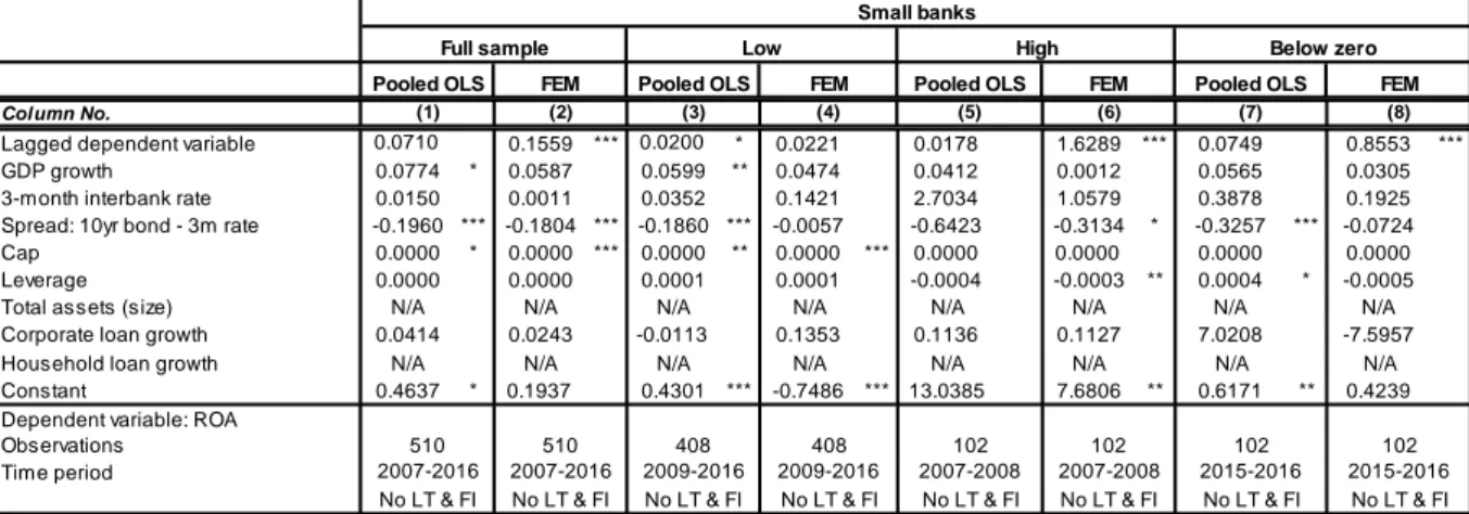
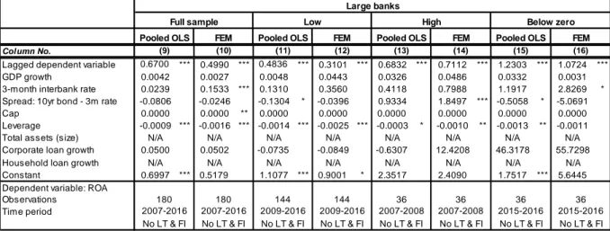
4.4.5. Mainregression results for small and large cap banks by low, high and below zero interest rate environment ... 34

5.

Analysis ... 36

6.

Conclusion ... 39

7.

References ... 41

List of Tables

Table 1. Different model variations ... 24

Table 2. Different model variations (2) ... 26

Table 3. Pooled OLS vs. FEM regression results by low, high and below zero interest rate environment... 28

Table 4. Pooled OLS vs. FEM for small cap banks by low, high and below zero interest rate environment... 30

Table 5. Pooled OLS vs. FEM for large cap banks by low, high and below zero interest rate environment... 31

Table 6. Regression results by low, high and below zero interest rate environment . 32 Table 7. Regression results for small and large cap banks by low, high and below zero interest rate environment... 34

List of Appendices Appendix A. Summary of banks found ... 46

Appendix B. Low and negative interest rate environment ... 46

Appendix C. GDP growth rate over period 2006-2016 ... 46

Appendix D. Summary statistics of the variables ... 47

Appendix E. Unit root tests ... 48

Appendix F. Variables plotted over the period 2006-2016 ... 49

Appendix G. Panel data tests for unit root ... 53

Appendix H. Covariance matrix ... 54

1. Introduction

In this part, we will present the subject on which this thesis is based on. A brief background will be given, together with the problem and purpose of the thesis and the delimitations we encountered.

1.1. Background

Since the global financial crisis of 2008, interest rates have been decreasing all over the world. In the period around the middle of 2014, in order to help economies recover, some central banks, including European Central Bank (ECB), have set interest rates below zero level. This decision affected not only firms and individuals, but also banks which provide services in the Euro area. Since commercial banks play a crucial role in the financial system and the economy, it is important to ensure good operating conditions for them. However, over the last few years, banks’ profitability indicators have been quite low or even negative and this might have been related to low short-term interest rates policy (Ongore, 2013).

Many studies confirm that low interest rates negatively affect banks’ profitability, because low interest rates are usually associated with lower net deposit margin (the difference observed between the lending rate, also known as the market rate, which is the bank's revenue, and the interest rate paid for the funding of this lending, known as the deposit rate and is the cost the bank endures). The relationship between interest rates and net interest margin can be explained by the simple consequence of a situation when central banks decrease the interest rate, which as a result leads to commercial banks having to decrease their market rate but not wishing to decrease the deposit rate at the same proportion, which as result increases the spread. This increase occurs due to fear the banks have that if the rate offered by them will be deemed to be too low in comparison to alternative sources of investment considered to be on the same risk level (for example long-term government bonds) then the depositors would prefer investing elsewhere. If this occurs, the banks would lose their main source of what was considered cheap capital, which would have been utilized to provide all the loans and hence they will not have the necessary tools to generate their profit from their main revenue making activity. Since, the cash flows commercial banks receive from investment in securities and investments minus interest payments on deposits directly depends on the interest rate (Morris & Regehr, 2014), it is common to observe a positive relationship between banks’ net interest income and the level

of the interest rate. Finally, affecting banks’ profitability, low or even negative interest rates might also have a negative impact on financial stability.

1.2. Problem description

It is traditionally believed that through interest rate cuts the economy should be boosted because of the higher corporate and household credit demand contributing to a minor loan growth (Jobst and Lin, 2016). This in turn should mitigate the negative effect of low interest rates on bank profitability, as the increased loan growth should balance out the loss the banks experience through the interest spread squeeze. This in particularly relevant to the euro area countries as these are perceived to have a high share of floating rate loans and a high dependence on deposit funding. IT has been observed that the expected loan growth did not occur when the interest rates have been lowered and thus the losses associated with the negative effect of low interest rates have not been covered, and as a result, the banks in the euro area have been burdened with weak profitability. Moreover, in the data period analysed (2006-2016), it can be observed that the banks in the euro area have made a decision not to expose firms and households to a negative deposit rate, as a consequence, falling market interest rates have not been followed by an equivalent lower deposit rates, meaning that the net interest margin has been squeezed (Monetary Policy Report, 2016). Yves Mersch, who is a member of the Executive Board of the ECB, admitted in his speech (published by ECB, 2016), that negative interest rates in the euro area will probably decrease the profitability of banks over the next five years, in some cases as low as 2% from 6.5%. As low interest rates could lead to the financial imbalances, particularly in more indebtedness and more credit as well as liquidity risk, this paper will focus on how the low interest rates and loan growth affect banks’ profitability.

The problem of this paper: what is the impact of unusually low interest rate environment and

loan growth on the soundness of the euro area banking sector in terms of profitability.

Our paper will contribute to the literature by further exploring the relationship between the unconventional monetary policy, specifically the low interest rate and bank profitability. We will be analysing annual data ranging from 2006-2016 which will also cover the period from middle of 2014 when the negative interest rate has been implemented, hence expanding the already existing literature on the subject, which does not as yet cover this period. In addition to this, we will extend the model to include the issue of loan growth, the importance of which has been briefly mentioned and is discussed further below.

1.3. Purpose

The purpose of this paper: to investigate in depth whether the low interest rates have had a significant effect on banks’ profitability in the euro area. Further extending our understanding in this field by also looking at loan growth and observing how this determinant also influences profitability.

1.4. Delimitations

There is an extensive amount of literature of many theories mentioning various external as well as internal factors which have an impact on bank profitability. However, in order to obtain meaningful results on the link between bank profitability, loan growth and the level of interest rate, only most significant and commonly used variables will be taken into consideration.

1.5. Disposition

The paper will be structured as follows: the next section will provide an overview of the literature on variables of bank profitability. Section 3 will present the data and the relevant variables for the empirical study on the euro area banking sector. Also, the model will be specified describing the methodology and the econometric techniques which will be used to estimate this model in search for consistent and reliable estimates. Subsequently, the empirical results will be presented, interpreted and discussed. Section 6 will provide limitations and a conclusion.

2. Literature Review

Bank profitability is often described as a function of both internal and external factors. The internal determinants of bank profitability usually consist of bank-specific factors such as size, capital and leverage ratio. The external determinants of bank profitability are on the other hand associated with outside environmental such as macroeconomic forces. The macroeconomic variables commonly analysed are interest rates and the growth rate in the economy. Various studies throughout the years study the different determinants which are important and affect bank profitability, which do not all agree and have the same findings. Despite the differences in arguments and results, we have found that all the below mentioned variables are quite important to be considered, when studying profitability of the banks.

2.1. Interest rate

Firstly, it is important to have a look at the effect of low interest rates to net interest income, which is considered to be the main source of earnings for the commercial banks. The interest rate plays a key role in controlling the level of inflation. In general, it is considered that the lower the interest rate, the more people are able to borrow therefore there is more money circulating in the economy and as result it can cause an increase in inflation as well as the economic activity (Gazioglu & McCausland, 2009). The opposite holds true when the interest rates go up where with less spending, the inflation decreases, and the economy slows. When negative or near zero interest rate policy was implemented by the central banks, commercial banks adjusted their lending rate accordingly. Since it can be observed that banks are highly reluctant to impose negative interest rates for depositors, low and negative interest rates set up by central bank should then lead to a lower interest margin, and thus banks’ profitability will get affected. However, because there are other factors which determine bank profitability, the direct effect of interest rate changes may not be as easily observable. According to Sveriges Riksbank, (2016) examples of such factors are loan volume variations, falling lending rates, credit losses and commission income. Therefore, there is a small but a fast-growing amount of literature on the effects of low or negative interest rates on bank profitability which will be briefly discussed below.

Alessandri and Nelson (2015) analysed UK banks, additionally including data of building societies and small retail entities which are similar to the cooperative banks and credit unions, over the period 1992 Q1 to 2009 Q3. Their study was based on the fixed effect model and GMM

approach adding bank specific variables, for example, a leverage, defined as the ratio of debt to total assets, and macroeconomic indicators such as the growth rate of GDP. They confirmed that there is a positive relationship between bank profitability and the level of interest rates in the long-term, however, in the short-term, the impact of higher interest rates can be negative due to repricing and yield curve risk. The studies showed if market rates decline by 100 basis points, the net interest margin goes down by 0.035% and 0.016% for commercial banks and building societies respectively.

Another research about banks’ net interest margin and the level of interest rates was made by Busch and Memmel (2015). To be able to differentiate between the short- and long-term effects of a rise in the interest rate level, they collected more than 40 years of dataset. They proved that the increase of interest rate level leads to an increase of the bank’s net interest income over the medium and term horizon and confirmed that the short-term effect and medium to long-term effects on banks’ net interest margin differ. It showed that if the interest rate level rises by 100 basis points, the net interest margin goes up by approximately 7 basis points. Also, it was noticed that due to low interest rate environment, the retail deposit margins have decreased by up to 97 basis points.

Moreover, Borio, Gambacorta, and Hofmann (2015) also did an investigation on how monetary policy affects bank profitability. Their study was based on cross-country data of 109 large international banking groups located in 14 advanced economies from 1995 to 2012. The authors used the yield curve slope (the difference between 10-year government bond yield and 3-month interbank rate) in order to demonstrate how unconventional monetary policy affects bank profitability. The analysis showed that short-term interest rates and banks returns have a positive relationship. They confirmed that at lower interest rates levels, the net interest margin effect is stronger (at a rate of below 1%, 50 basis points for 1% change was observed) than at higher interest rates levels (20 basis points change at a rate of approximately 6%). Furthermore, both net interest and non-interest income responded to the level of the short-term rate and the yield curve slope positively, meaning that this is concave (non-linear) relationship. Finally, Borio, Gambacorta, and Hofmann (2015) noted that due to non-linearities of low interest rates and flat term structure, rate cuts (if starting from already low levels) might diminish bank profitability significantly.

One of the latest research about “Low-For-Long” interest rates and banks’ interest margins and profitability was done by Claessens, Stijn, Coleman, and Donnelly in 2017.Using a sample of 3,385 banks from 47 countries for the period 2005-2013, they confirmed previous studies results that low interest rates, comparing to high interest rates, have significantly higher impact on banks net interest margin. According to the authors, the impact on net interest income is greater than on net interest expense and also banks which have long-term investments in their balance sheets are less affected by the change than the banks which rely more on the short-term investments. They found that a one percentage point decrease of interest rate leads to a drop of lower net interest margin by 8 basis points, with this effect greater (20 basis points) at low rates. Moreover, net interest margin and bank profitability decreased accordingly by 9 and 6 basis points. Finally, it was suggested that, in order to mitigate a negative low interest rate impact on banks’ profitability, banks should cut their costs and focus on generating higher non-interest income.

In contrast, Riskbank’s Monetary Policy Report (2016) claimed that major Swedish banks had reported high and stable profits during the interest rate cuts in recent years due to the high cost efficiency and low funding costs. The cost-to-income ratio of Swedish banks decreased from 51% to 47%, while in other European countries, it went up from 62% to 74% during the period from 2009 to 2016. Turk (2016), is an example of another investigation about profitability of Swedish and Danish banks in a context of negative monetary policy rates. According to the author, even though there has been some compression of margins between banks’ lending and deposit rates, the banks’ profitability has remained stable. The high levels of profitability were explained by non-deposit funding and historically low interest expenses. Also, Danish commercial banks have raised their profit by non-interest income, such as fees of mortgage refinancing as well as advisory services to corporations. Therefore, observation of bank activity in such countries could be an example of the actions to be taken and alternative methods to consider, in order to maintain the profit for the banks in the Eurozone.

Genay and Podjasek (2014) argue that the effect of near zero interest rates on banks’ bottom line has been covered by boosted economic activities such as higher lending volumes and the better performance of existing loans. Their study showed that even though the low interest rates have resulted in the banks earning slightly less for every dollar lent because the interest rate on deposits has not fallen as much as the market rate, the direct effects of negative or low interest rates on banks’ profitability have low economic significance. On the other hand, they found out

that the level of house prices and unemployment rate had a greater effect on banks’ profitability than declining interest rates. For instance, if an unemployment rate decreases by 1 per cent, return on assets increases by 9 basis points, which is six times larger effect than the effect of change in short-term interest rates. Similarly, the increase of 1% in house prices decrease bank profitability by 5 basis points.

However, a decline in the profitability of banks linked to an adaptive monetary policy may lead to a less stable banking. According to Rajan (2005) a former Governor of the Reserve Bank of India, who described a process in which changes in interest rate policy could affect risk-taking, if lower interest rates on bank’s short-term assets are implied in comparison to the long-term obligations held on the balance sheet, banks might tend to accept higher risk switching from low to high risk assets. According to that, it is worth mentioning that when analysing both euro are and U.S. lending standards, some evidence was found out that low short-term interest rates soften lending standards rather than low long-term interest rates. Due to low interest rates policy, high securitization as well a weak supervision of a bank’s capital, banks are willing to take higher risk which could lead to the financial crisis (Andries, Cocris, Plescau, 2015). Riskbank also agreed that the current situation of the large exposure of the banking sector to the housing market (in the context that house prices and the high level of household indebtedness associated with that increase very fast) is very challenging and needed to be closely monitored.

2.2. Loan growth rate

Not many studies took into consideration loan growth rate as a separate variable. However, it is mentioned in some studies as an important factor for bank profitability. From theoretical point of view, the impact of growth of a bank’s loan volume changes is quite difficult to predict. For instance, it can be expected that if the bank has a higher loan growth rate (comparing to the market’s growth rates), this bank will be considered to be more profitable compared to the others, as it will have performed better than the market. However, if this is achieved through lower interest margins then it can be expected that this may have the opposite effect and actually have negative influence on profitability. Moreover, high growth of loans might also lead to a decline in credit quality as well as higher levels of non-performing loans and thus to a lower profitability (Dietrich and Wanzenried, 2010). For example, during the crisis, the return on equity (ROE) of European banks with the highest loan growth rate (between 2003 and 2006) declined to 6.77% in 2008 from 13.34% in 2006, while the ROE of banks which had lower rate

of loan growth decreased less sharply from 10.46% to 5.65%. The interesting fact is that the profitability of banks with lower loan growth rates increased, while the ROE of banks having high growth of loan volumes declined further in 2009.

These occurrences have been further explored by various studies, for example Demertzis & Wolff (2016) recognise that the diminished margin only gradually affects the income derived from net interest which can be compensated by an increase in fees. This is because this decrease in the spread only mainly affects new loans and if the loan growth rate is low, the effect will not be visible for some period of time. Additionally, Jobst and Lin, (2016) state that low growth of loans, may also make it harder for banks to balance out the profits in net interest earnings from the impact of declining margins. In other words, higher frequency is required to maintain the profitability of the banks due to the fall of the margin. Borio, Gambacorta & Hofmann (2015) also recognize the fact that bank profitability loss through lower loan levels can only be observed in time, as lower interest rates should encourage loan growth which will cover the negative effect. Dietrich and Wanzenried (2010) recognised the importance of loan growth and included the difference between bank and market growth of total loans as a separate variable as a determinant of bank profitability. Given that the effect of loan growth could have opposite consequences, the overall relationship with bank profitability has yet to be determined and this is what we would like to try and obtain empirically.

2.3. Other factors

Finally, when analyzing the relationship between bank profitability and low interest rates in the low loan growth environment, it is also important to consider other factors that the researchers found to have a significant effect on the profitability of the banks. Using the example of a study conducted by Staikouras & Wood (2002), who researched what the determinants of European bank profitability are, they have found that the European banks profitability depend on external macroeconomic environment and the bank related influences such as bank leverage ratio, loans to assets ratio and market share of the banks. Other studies have found alternative variables which were seen as significant to consider when running such models. Therefore, the rest of the literature review will be based on other factors we implemented in the model and the reason why we saw it was important that they were included.

2.3.1. Economic growth

It has been addressed that the profitability of the banks also depends on external macroeconomic environment such as GDP growth rate (the most used measure of economic performance of a country) which has a positive relationship with bank profitability (Demirgüç-Kunt & Huizinga (1999), Albertazzi & Gambacorta (2009) and Bikker & Hu (2002). In favourable economic conditions, meaning when the GDP in growing and is perceived to maintain this trend, the demand for credit by households and companies is higher, which improves the profitability of the banks. Furthermore, Bolt et al. (2012) state that in economic booms the level of credit risk is believed to be lower, which lowers credit loss necessities and directly boost profits. To confirm this from the other perspective, Flamini, McDonald & Schumacher (2009) state that as the growth of economies slows down or even enters a recession, the result is an increased number of non-performing loans and thus lower profitability for the banks. However, Borio, Gambacorta & Hofmann (2015) findings convey a weak correlation between GDP growth and net interest income and no correlation at all between GDP growth and non-interest income. On the other hand, Claessens, Coleman & Donnelly (2017) when performing a cross-country analysis of bank profitability found that the coefficient on GDP growth is insignificant in the low and significantly negative in the high interest rate environment. Therefore, from previous studies there appears to be a mixed view on the relationship between these two factors.

2.3.2. Bank size

Another variable which has opposing views on its effect on bank profitability is the bank size. Demirgüç-Kunt & Huizinga (1999), Goddard et al. (2004) and Borio et al. (2015), Redmond & Bohnsack (2007) find a positive effect between the two, whereas Aladwan (2015) convey that bank size has a significantly negative effect on profitability. Bertay et al. (2013) argue that the positive relationship declines with systemic importance of the bank and the fact that a possible explanation for this fact is the “too-big-to-fail” perception of these bigger and more important banks. On the other hand, Arif, Khan & Iqbal (2013) found a mixed relationship which varied depending on initial size of the banks. Which is further supported by Athanasoglou et al. (2006) and Trujillo-Ponce (2013) who found an insignificant effect and suggest a non-linear relationship such that profitability initially increases with size and then declines. Redmond & Bohnsack (2007) explain that one of the possible reasons why one should expect to find a significant relationship between bank size and bank profitability, is because banks of a larger size are expected to have the ability to increase the scale and scope of their activities as necessary. Short (1979) states that larger banks can create capital cheaper than small banks,

which implies that larger banks have the possibility to earn greater profits. However, this would suggest that the relationship between bank size and profitability should always be positive.

2.3.3. Bank leverage

Dell'Ariccia, Laeven and Suarez (2013) found a negative relationship between the interest rate and bank leverage. With an interest rate cut bank monitoring is lowered and increase risk taking occurs which is related to greater leverage, which in turn tends to increase the profits. Staikouras & Wood (2002) have performed one of these researches on the determinants of European bank profitability. Pagratis, Karakatsani & Louri (2014) argue, banks may be willing to take on high levels of leverage, when risk premium is low, to maintain their returns the Basel III requirements, that have been implemented from 2013, have mainly increased the capital requirements of banks and have set a minimum leverage ratio to 3% in order to make the overall banking sector more stable.

2.3.4. Bank capitalization

Bank capitalization, is another factor influencing bank profitability. Mahapatra (2012) a report analysing Basel III changes, states that these increases in capital requirements may negatively affect bank profitability. Demirgüç-Kunt & Huizinga (1999), Moussa & Aymen (2013), Borio et al. (2015) to name a few, have all found a positive relationship between bank capital and profitability. (Iannotta et al. (2007) even suggest that banks with riskier assets may be perceived to have higher capital levels. Olivier, Camara, Pessarossi & Rose (2014) show that through higher returns, bank can obtain higher capital ratios which in turn could yield higher profits. Athanasoglou et al. (2008) found that bank capital acts as a protection basis in the case of hostile events, allowing the banks to sustain their profitability in economically difficult times.

To sum up, the main literature concerning the interest rates and loan growth rate effect on bank profitability as well as other determinants has been discussed. Following the detailed analysis of previous studies, an appropriate research methodology was formulated and applied.

3. Methodology

We begin this section, by introducing the hypotheses we tested, following on by defining the data utilised and the model the whole analysis was based on. Here also a description will be given, of the various approaches used in the analysis of the problem.

3.1. Hypotheses

The hypothesis that we have tested in the empirical part of the thesis is to find out whether low interest rates indeed do have a significant effect on the bank profitability in the Eurozone. Further to this, as we have also implemented loan growth into the model, the other hypothesis we tested was whether this addition was accommodating and if both of these variables simultaneously as well as separately had an effect on bank profitability in the Eurozone. Therefore, our testable null hypotheses are whether low interest rates do not significantly affect bank profitability and if loan growth rate does not significantly affect bank profitability.

3.2. Data

In this thesis, annual data for 72 banks from different countries from the Eurozone was collected to represent the whole euro area for the period from 2006 to 2016. There are some reasons why we chose to study the Eurozone. First of all, Euro area is considered to be a small stock market because of its size in comparison to other stock markets seen in the world but at the same time it has a large volume of bank loans. Therefore, countries in the Eurozone could be thought of as bank-based countries, and, following this, it is very important to investigate what determinants significantly influence the banks’ profitability in this region (Allen & Carletti, 2008). Secondly, from 2006 to 2016, the interest rate environment in Eurozone has changed from normal or even high (pre-crises period) to low or even negative (post-crises) environment, therefore, making it a unique and interesting area to analyse. Finally, there had been some criticism with regards to European Central Bank, mentioning that since there are too many country specific factors, it does not always coordinate its monetary policy efficiently (Srivangipuram, 2013). Therefore, we would like to elaborate on how the low or even negative interest rate policy has affected the banks’ profitability in these areas.

The number of bank information collected from each country can be seen in the Appendix A. All data was collected from DataStream from the publicly listed banks of the consolidated financial statements. We did take note that these performances are not pure identifiers of the

performance solely in the euro area as these banks could have branches in countries outside the Eurozone. However, as their head offices are in the Eurozone, it is assumed that these banks’ main operations are conducted in this area and therefore the results should still be significant and applicable. Unfortunately, DataStream did not have data available for some countries (Estonia, Latvia, Luxembourg and Slovenia) in the Eurozone, therefore some countries will not be in the analysis. We believe that this should not have an impact on the study; firstly, Estonia, Latvia, Luxembourg and Slovenia are relatively small countries representing only 1.3% of total euro area GDP. Also, since they are small countries, they either do not have publicly listed large local banks at all or even if they do have, there are not many. Finally, the target was to obtain as many banks as possible from the Eurozone as an area and capture the whole picture as well as the main trend in the area and not the particular situation of each individual country. The euro area banking interest rates are dictated by the ECB in most countries and the loan growth rate used is also a general rate observed in Europe.

The other factors taken into consideration allowed us to control that banks functioned in different circumstances, thus individual bank influences were also taken into consideration when running the analysis. It is useful to note, that for some model analysis, sometimes banks from a particular country, which did not fit into the criteria being analysed, were taken out of the sample. For example, when we analysed variable in low and high environment, Lithuania (1 bank) and Finland (2 banks) were taken out from the sample because they do not agree with the criteria of 3 months interest rate being below 1.5% in 2009 and then Finland also did not lower their interbank rate below 0% in 2015 (Appendix B). Also, when we tested different models in order to see how results vary to see how we can improve our model, we noticed that Greece, Lithuania and Ireland were the outliers in GDP growth variable (as can be seen in Appendix C) and for this reason they were excluded for that particular analysis.

3.3. Model

The model was built based on the models used in the studies conducted by Borio, C., Gambacorta, L. and Hofmann, B. (2017) and Claessens, S., Coleman, N. and Donnelly, M. (2017),adding on the loan growth terms in accordance to the hypothesis we would like to test. We decided to base our model on these papers as we wanted to see whether their results, which were on a more international level analysis, would be similar and applicable to a smaller sample of the Eurozone. We carry out the econometric analysis using the following benchmark model:

Y_i,t= α₀+ α₁Y_i,t−1+ βr_i,t+ γRateSpread_i,t+ δGDPgrowth_i,t+ ςCLG_t+ ϕHLG_t+ ψSize_i,t + θLev_i,t+ ζCap_i,t+ τX_i+ ρD_1t+ μD_2t+ ε_i,t

where i represents the various samples used in the study which are the different banks and t is the time span across which the model is applied.

• Yi,t is return on assets;

• Yi,t−1 is the first lag of bank profitability;

The monetary policy indicators are represented by:

• r_i,t is the three-month interbank rate;

• RateSpread_i,t is the difference between the ten-year government bond yield and the three-month interbank rate;

Macro controls:

• GDPgrowth_i,t controls for the country’s economic growth;

To represent loan growth:

• CLG_t is corporate total loan growth rate in euro area; • HLGt is household total loan growth rate in euro area;

In order to take into account bank characteristics, we include a set of bank-level controls:

• Sizei,t– bank total assets;

• Levi,t – bank leverage debt-to-equity ratio;

• Capi,t – bank book-to-market ratio;

Other:

• Xi is a bank fixed effect (the deviation from the intercept for each bank covering the

other bank effecting variables not covered in the model);

• D_1t is a dummy equal to 1 for low interest rate environment from 2009 to 2014; • D_2t is a dummy equal to 1 for the negative interest rate environment from 2015 to

Finally, ε_i,t is just the error term at a current time period.

Since the return on assets was not available for all the banks for all years in DataStream and in order to have a more consistent number, the variable was calculated manually as the ratio of its net income in a given period to the total value of its assets. The financial leverage ratio was calculated by dividing the total debt to the total equity and the bank book-to-market ratio is the common shareholder’s equity divided by the market capitalization. All the ratios were then multiplied by 100 and thus all variables except size were expressed in percentage terms. To make interpretation of the size variable results easier, total asset variable was transferred to the natural logarithm form. Nevertheless, diagnostic checking was conducted on both size as a total asset number and size as a natural logarithm, in order to see whether the results differed. A detailed summary of the statistics for each variable can be found in Appendix D.

Furthermore, note that the equation included the first lag of banks’ profitability. This is because it was believed that bank profitability in the current year should highly depend on the profitability in the previous year since loans which were provided by the banks to the customers in the past are more likely to be longer than one-year term loans and thus they should generate cash flows for some time in the future. Besides, according to Afsar, Rehman, Qureshi & Shahjehan (2010), the lagged dependent variable should have been included also based on customer loyalty in the banking sector, they were basically stating that cash flows of operations provided to the customers at the current period should also depend on the cash of operations provided in the previous period. And finally, by including the first lag of bank profitability, we diminish the potential problem of omitted-variable bias.

3.4. Method

To begin with the raw data was categorized for each bank, meaning that when there were variables where the macroeconomic data was representing the situation of an individual country or area, these were implemented to each bank accordingly to where the bank is located and as a result for each variable the data was stacked in columns corresponding to each specific bank in the specific year.

3.4.1. Unit root testing

Following this, before running the model discussed above, prior testing of the data was conducted. If we use the data without checking whether it is stationary, the problem of so-called

spurious results might occur (Datta and Kumar, 2011). Therefore, it is very important to conduct a unit root test to see if one of the main required assumptions with regards to the variable being stationary, is held true. After the introduction of testing of panel unit root by Levin and Lin (1993), a few more tests have been determined, for example, Eviews offers five different tests two of which assume a common unit root: Breitung (2000) and Levin, Lin & Chu (2002), and three tests with the assumption of individual unit root process: Im-Psarian-Shin (2003), Fisher-type tests using ADF and PP tests (Maddala and Wu, 1999, and Choi, 2001), (Schwert, 2015) and they are briefly discussed in the Appendix E. Common unit root implies that the same event has an influence on all the observations at hand, which is quite probable in our data analysis.

Therefore, the procedure for testing this was as follows: at first, the graph for each variable over time was plotted in order to see whether the mean was reverting as well as if variance was growing/declining to infinity or not. If it was observed that mean, variance or covariance deviated from the constant mean, then an intercept needed to be included in the test, and if a variable was growing or shrinking in the long-run, then an equation with individual intercept and trend was to be estimated. This approach is very significant, because if the trend term is mistakenly omitted, the tests are biased toward finding a unit root. However, as it can be seen in graphs in the Appendix F, the panel data was difficult to interpret, therefore, we followed a simplified unit root model selection strategy approach based on Elder’s & Kennedy’s (2001), when a variable’s growth status was unknown. This strategy had two steps to follow: at first, unit root tests with an individual intercept and trend were applied. If the null hypothesis was rejected (where H0: ρ=1 (unit root) against H1:ρ<1 (no unit root)), the p-value was lower than

5% significance level, we could conclude that there was no presence of unit root in the variable. However, if the null hypothesis could not be rejected, unit root tests with intercept only were applied in order to identify whether there was a drift (stochastic trend) in the data or not, as we could not conclude if the variable was growing or not. If the null hypothesis could not be rejected in the second step, we concluded that a variable is not stationary and, to avoid a spurious regression relationship, then the first difference would have been required. However, it should be mentioned that the results of such regression would have been hard to interpret in our case as the data definition would have been completely altered. Also, in such circumstances long-run information disappears and thus it is mostly suitable when only interested in the sign of the coefficient (negative or positive) and not the coefficient value obtained.

However, it is necessary to mention that there are some disadvantages of testing unit root for panel data. The main limitation of these tests is that they are all formulated under the assumption that the individual time series in the panel are cross-sectionally independent, when on the contrary, there is considerable evidence of the co-movements between economic variables (Choi (2002) & Pesara, 2003). Ignoring cross-sectional dependence in unit root estimation could lead to a loss in efficiency of the test as well as invalid test statistics (Schwert, 2015). Moreover, unit root tests for the panel data are difficult to interpret, for example, although both Levin, Lin & Chu and Im-Pesaran-Shin tests (further described in the Appendix E) have the same null hypothesis, it is not possible to have a straightforward comparison between them, since the alternative hypotheses are quite different.

It is also worth to mention that Kao (1999) revealed that estimates of the structural parameter binding two independent non-stationary variables converges to zero in the case of panel data, whereas in the case of time series it is a random variable. This means that although non-stationary panel data may lead to biased standard errors, the point estimations of the value of parameters are consistent. As regardless of the outcome with regards to the stationarity level of the variables, the model with panel data variables could still be conducted at level and provide meaningful results. Following this, we based our analysis on variables at level. However, we also took into consideration that some of our variables are non-stationary and for comparison reasons, in addition to our main analysis, we ran the regression based on first differences to see whether the same variables have significant impact on banks’ profitability and the same positive or negative relationship was maintained.

3.4.2. Correlation testing

A further test we considered was the correlation between the variables, to ensure that the proposed model was robust and parsimonious. If high correlation was present between some variables it could be concluded that there is no need to keep both of the variables when conducting the regression as the effect of the inclusion of the extra variable should be covered by the correlated variable. If both variables were to be kept in the model, correlated variables would lead to multicollinearity problems, which increases the standard errors of the coefficients (Chatterjee & Hadi, 2013). Overinflated standard errors, would make some of the variables statistically insignificant when they should be significant. It is sometimes a difficult choice which variable to eliminate from the regression, especially if the theory suggested that both variables are important in determining an outcome. However, this issue is not applicable if both

variables basically represent the same factor; hence by observing that they are indeed similar it does not cause a problem to the model to remove one of them.

3.4.3. Granger-causality testing

To further analyse how well the suggested model was built, we looked at the Granger causality between each of the variables. According to the Granger (1969) causality approach, if x helps in the prediction of y, or equivalently, if the coefficients on lagged values of x are statistically significant, it means that x Granger-causes (or “G-causes”) y. Therefore, in this paper, in order to find out how well the suggested model was built, we looked at the Granger causality between each of the variables to ensure that indeed all the suggested variables had a relationship with either the dependent variable ROA or the main tested variables which included spread, interbank rate or loan growth based on the theories discussed previously. To test for this panel causality test of Dumitrescu and Hurlin (2012) was used, which is advised to be applied when there is a large number of observations which could be increased, and time observed is constant. Moreover, this test is based on Vector Autoregressive models (VAR) and assumed that that disturbances in panel data models are cross-sectionally independent. However, the Monte Carlo simulations have been known to show that even under the conditions of cross-sectional dependency, strong results can still be produced. This test can be used for balanced and heterogeneous panels, taking into account two different dimensions: the existence of the individual effects between individuals, or the existence of different intercepts. The null hypothesis states that there is no causal relationship between the variables and it was defined as follows:

H0: βi = 0, ∀i= 1, … , N (no Granger causality);

H1: β_i ≠ 0, ∀_i= N₁+ 1, N₁+ 2, … , N (Granger causality).

3.4.4. Model selection: pooled OLS vs. FEM

Following this, the analysis of the data was conducted, running the regression on the basic model and then adjusting it by taking different findings and circumstances into consideration and observing how these changes were affecting the results. To begin with, pooled regression model was run also known as the constant coefficients model, which assumed that the same intercept andsame slope was appropriate for all the observations; meaning that coefficients remained constant for all the banks and over time, which is a very strong assumption that does

not control for heterogeneity in the data. However, it was useful to run this regression to have it as a baseline comparison model, therefore for all further adjustments, the pooled regression model was also conducted as a starting point. Then, using the same model, a regression with fixed effects for cross sections was done. This meant that we were assuming that the slope coefficients were equal over the cross sections, which is in our case meant over the different banks but allowed for these countries to have different intercepts. This is quite a probable assumption considering the data we have, we expected for the bank data to have similar slopes but because of the various circumstances they operate in, it is logical to assume that the intercept for them would be different. Following this, we ran a redundant fixed effect likelihood ratio test, to consider whether the fixed effects model (FEM) is indeed required for the regression or whether the pooled regression would suffice. The null hypothesis in this case was whether the fixed effects are redundant, and should not be used, therefore if the resulting F-test was below the 5% significant level it would convey that the null hypothesis was rejected, and the fixed effect restrictions were supported by the data thus a pooled regression could not be used.

3.4.5. Model selection: FEM vs. REM

Ensuing the above, we tried to run a regression where there was a fixed effect for period implemented into the regression, which would assume that the intercepts were different over time. Thus, implicitly this meant that the intercepts are equal across cross sections. This assumption was not a very realistic one, because as mentioned before, the banks in the sample were firstly different in themselves, for example in their size and they were also operating in slightly varying economic conditions. In addition, we did not expect to see a severe change in the intercepts as time varied from year to year, but more from period to period, which is connection to the dummy variables included in the model. The final regression type conducted was the assumption of the random effects for the cross sections, where it was also assumed that the intercepts were different for the banks, but slope coefficients remained constant over the various banks. It is commonly perceived that where the sample consists of a large number of observations over quite a short period of time that the random effects model (REM) is more appropriate than FEM. However, if the errors and the observations are correlated, then the FEM is more appropriate as then the results obtained from the REM are meaningless. This can be determined by the Hausman test, which was also conducted to check whether the results obtained with the REM could and should have been taken into consideration.

3.4.6. Model variations

Apart from the basic model presented above, further variations of the model were done, and their results compared to obtain a deeper understanding of the effect interest rates have on the profitability of the banks. This included analysing the banks performance in high, low and below zero interbank interest rate environment; separating the banks in accordance to their market capitalization and running isolated regressions for large and small cap banks; and also, a regression where countries which acted abnormally in comparison to the trend seen in Eurozone with regards to the GDP growth were taken out to analyse if this altered the results in any way. We also conducted our regressions, where correlated variables were taken out in order to have a more parsimonious model. To verify the necessity of inclusion of the loan growth into the model and its effect on profitability, various regression alterations were made, for example, where the main variable analysed was loan growth without including spread or interest terms or even both of them and also models where loan growth variable was not included at all to test whether not including this variable made an impact on the results.

4. Results

In this part, the results of the empirical analysis of the data, different models and the hypotheses raised, will be presented. As per the methodology, we first give the results of the unit root testing correlation and causality between the variables. Secondly, we present the results of the differences in value, significance and sign between the various alterations of the model tests. Also, the differences in results between the basic pooled OLS and the fixed effects models. Finally, we interpret the findings of the regression analysis in low, high and negative interest rate environment and further for the different cap size of banks in these three periods.

4.1. Unit root results

The results of unit root tests in the Appendix G showed that all p-values of banks’ profitability (in our case return on assets) GDP growth as well as leverage for all unit root tests were lower than 5% significance level and the null hypothesis could be rejected. Therefore, we can say that these variables did not contain unit root and were stationary at level. However, the results differed for the rest of the variables. When testing book-to-market ratio at level with individual intercept and trend, we could see that all the tests except Breitung t-stat showed no unit root in the variable. Nevertheless, even though the only one test out of five showed unit root, there was still a possibility of random walk being present in the data. Therefore, the tests with intercept only was applied. Since all the tests had probabilities lower than 0.05, the null hypothesis could be rejected, and we could conclude that book-to-market ratio was stationary at level. Moreover, it could be observed that household loan growth variable also had a unit root when the intercept and trend were included in panel unit root testing, because 4 out of 5 tests has p-values higher than 0.05. When the tests with intercept only were applied, household loan growth variable also did not contain unit root and was concluded to be stationary at level. Furthermore, panel unit root testing with trend and intercept for the 3-month interbank rate, spread, corporate loan growth rate as well as size (total assets) and natural logarithm of size showed that there was a high probability of random walk in these variables. In addition, tests without trend were also applied and since most of the tests p-values were higher than 5% level of significance, we could reject the null hypothesis, meaning that the 3-month interbank rate, the spread, the corporate loan growth rate and the size (both as total assets and in natural logarithm form) had a unit root and were not stationary at level.

4.2. Correlation results

As discussed, at first the correlation and the causality between the variables was observed in order to distinguish on the basic level, how effective was the model we were suggesting running a regression on. The covariance matrix table in the Appendix H conveyed that corporate loan growth and household loan growth were very highly correlated at 0.94 meaning that these two variables followed a near enough same pattern of changes throughout the years analysed and hence should have the same effect on the dependent variable. This implied that in order to keep the model parsimonious, we should avoid using both variables, the result in itself was not surprising as it could have been expected that the two would follow a similar pattern. The correlation between household loan growth (HLG) and 3 months interbank rate was 0.86 and similarly the correlation between corporate loan growth (CLG) and 3 months interbank rate was 0.82, with only a slight change observed. This could imply that possibly there is no need to include growth rate in the model at all, which would explain why most of the other models did not implement it into their model. In order to test our hypothesis with regards to loan growth we therefore have conducted an analysis with different variations in connection to inclusion and exclusion of loan growth in the regression. Based on the theory as previously discussed, the positive correlation number seen goes against the general expectation, that lower interest rates would, as a consequence, lead to higher loan growth; which further confirms that other factors affect loan growth and the relationship between these two factors is more complicated. As the correlation number is not extremely high, we still believed that loan growth should be included in the regression model. It has also been noted that bank book-to-market ratio and size correlation was as high as 0.76, which could imply that one of the variables was not necessary in the model which we analysed further with causality.

4.3. Granger-causality results

We next examined the relationship between the variables to confirm that indeed these variables were somehow interconnected and hence it was important to include them in the model. The table in the Appendix I shows the main findings which were related to the prior theory and discussion. The main finding in this table was that controversary to the previous findings, in our case the size of the bank (in natural logarithmic form nor just as total assets) were not significant in determining the ability to make and maintain profit, nor was it influencing any of the other important variables, as in all the cases the zero hypothesis was accepted. Therefore, further to the correlation issue above between size and bank book-to-market ratio, it was decided not to include size in our regression analysis. The results also displayed that only GDP

growth and spread had a direct influence on the profitability of the banks, which will be further perceived in the regression results once the regression is conducted. As we also had to make a decision which of the loan growth rates to eliminate from our model for the regression analysis, we believed that it will not make a large difference which ever one we chose as they were similarly affected by whatever outside factors throughout the years analysed. Therefore, since household loan growth exerted a slightly higher correlation with interbank rate, in causality testing it had a higher probability of a non-causality relationship with profitability and was perceived to vary slightly less than corporate loan growth, household loan growth was removed from the model. It was perceived that all the other variables were indeed somehow connected to the important variables in the model and hence confirmed the statement that these were necessary in order to control for the various exogenous factors influencing bank profitability.

4.4. Model results

Prior to discussing the results of the various regressions conducted, it should be noted that for most regression variations, the model with the fixed effect for cross-sections model (fixed effects model) was the preferred model over the pooled ordinary least squares model (pooled OLS), which was defined by the redundant fixed effect likelihood ratio test. The null hypothesis was rejected in all cases apart from the regressions where only the observations which followed the general GDP trend were used and when the regressions in first difference were conducted. This is the reason that for these regressions the pooled OLS results were displayed in Table 2 below, where the results for these regressions will be presented. Furthermore, when running the Hausman test it was concluded that the random effects model was not appropriate for the dataset we were analysing. Additionally, when trying to implement a fixed effect for period into the regression, a near singular matrix error would occur in all cases. This was also the case when we tried to run a regression with manually created time dummy variables for each year even when one of the years was taken off in order to avoid the dummy trap. The only way it could be done was to remove the intercept and all other variables from the regression equation, which provided meaningless results for our analysis. There are various possible reasons why this was the resulting issue when trying to run a test controlling for time effects, the main one we assume is that there were no major changes observed across the years, only more so across the different time periods, and therefore, we considered the model where these effects were controlled for by the two dummy variables we have included in our model. With regards to the lagged dependent variables, this was always taken out from one year back outside of the period being analysed, therefore the years shown in the results were actually the years the samples analysed

were based on. It is also worth mentioning that, since the fixed effects model was chosen as the main model for the analysis, only its regression results were interpreted and compared to the findings of the previous studies.

4.4.1. Model alterations

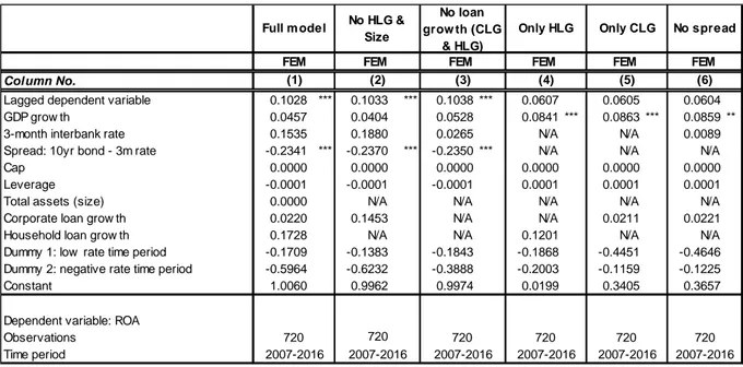
The first model we run a regression on, was the full model, where all the variables were included, just as a basis for comparison. As noted, the simultaneous inclusion of certain variables may raise concerns of multicollinearity and that is why we computed several tests in order to ensure that our results should not be affected by this issue. Following this, the two variables size and household loan growth for the reasons discussed above were taken out of the model. The results of these can be seen in Table 1 in columns 1 and 2. We see that not including the two variables did not alter the resulting coefficients by much and we still observe that only the lag of dependent variable and spread are significant. Taking into the example the significant coefficients, in column 1, spread was -0.2341 and a similar coefficient of -0.2370 was seen in column 2 and similarly the lagged dependent variable coefficient value was around 0.1030 in both columns. Bank book-to-market ratio, leverage and GDP growth also remained almost the same for both tests. Three months rate increased from 0.1535 in the full model to 0.1880 where the two correlated variables were taken out and the dummy variables values slightly changed from -0.1709 to -0.1383 and from -0.5964 to -0.6232 in columns 1 and 2 accordingly. Therefore, the results did not differ much, but we were saving 2 degrees of freedom by removing the two correlated variables. However, when taking out both corporate and household loan growth terms and, also, size, the significant variables remained the same and so did their value approximately, but the coefficient for the dummy variables for the low rate environment changed from -0.1383 to -0.1843 from column 2 to column 3 and for the below zero rate, quite excessively from -0.6232 to -0.3888 which implies that not including corporate loan growth will alter how the data in the low environment is perceived.

Table 1. Different model variations

Note. *, ** and *** denote significance at the 0.1, 0.05 and 0.01 respectively. Table made my authors (2018).

The other alternative variations of the model were based on the study conducted by Dietrich and Wanzenried, (2010) where their main model was similar to the one we propose, and they recognised the importance of loan growth, but it did not include interest rate and spread in their analysis. Consequently, we run models based solely on household loan growth (HLG) or solely on corporate loan growth (CLG), also without spread and rate and compared the results between these and column 2. Whether including only household loan growth or corporate loan growth, in column 4 and 5, we observed practically no difference in coefficient values for the first lot of variables and in both cases, lagged dependent variable was not significant but interestingly now GDP growth is. However, including one loan growth and not the other did influence the dummy variables and the intercept values; when only HLG was included the coefficient value for the dummy representing low rate period was -0.1868 (column 4) and -0.4451 when CLG only was included (column 5), comparing these to -0.1383 in column 2. For the below zero rate period dummy there was an even larger difference between the coefficients, where we observed the value -0.2003 in column 4 and -0.1159 in column 5 in comparison to -0.6232 in column 2. Also, the intercept value was 0.0199 and 0.3405, which is entirely different to column 2 where the coefficient value if the intercept was 0.9962. Also, when comparing the first variables to column 2, the results of both of these models were completely different in value and significance, an exception to this were the bank controlling factors variables, bank book-to-market ratio and leverage. Lagged dependent variable from the main model in column 2 fell from being significant at 0.1033 to being insignificant and with a value around 0.0606 in column 4 and 5. GDP growth was insignificant and 0.0404 in column 2 and became statistically

Column No.

Lagged dependent variable 0.1028 *** 0.1033 *** 0.1038 *** 0.0607 0.0605 0.0604

GDP grow th 0.0457 0.0404 0.0528 0.0841 *** 0.0863 *** 0.0859 **

3-month interbank rate 0.1535 0.1880 0.0265 N/A N/A 0.0089

Spread: 10yr bond - 3m rate -0.2341 *** -0.2370 *** -0.2350 *** N/A N/A N/A

Cap 0.0000 0.0000 0.0000 0.0000 0.0000 0.0000

Leverage -0.0001 -0.0001 -0.0001 0.0001 0.0001 0.0001

Total assets (size) 0.0000 N/A N/A N/A N/A N/A

Corporate loan grow th 0.0220 0.1453 N/A N/A 0.0211 0.0221

Household loan grow th 0.1728 N/A N/A 0.1201 N/A N/A

Dummy 1: low rate time period -0.1709 -0.1383 -0.1843 -0.1868 -0.4451 -0.4646

Dummy 2: negative rate time period -0.5964 -0.6232 -0.3888 -0.2003 -0.1159 -0.1225

Constant 1.0060 0.9962 0.9974 0.0199 0.3405 0.3657

Dependent variable: ROA Observations Time period 2007-2016 720 720 720 720 720 720 2007-2016 2007-2016 2007-2016 2007-2016 2007-2016 Full m odel FEM No spread Only CLG Only HLG FEM FEM FEM (1) (2) (3) (4) (5) (6) No loan grow th (CLG & HLG) FEM No HLG & Size FEM

significant with values of 0.0841 & 0.0863 in models only HLG and only CLG respectfully. Hence this confirmed that based on theory, spread and interest rate terms were indeed important factors to be included in the regression, and that their omission would completely alter the resulting outcomes.

For even further analysis, we tried to run a regression where the previously significant term was not included in our next regression, spread was omitted but we kept the interest rate in the model, and in this case the result was almost identical to what was observed in column 5 with corporate loan growth (as in this case, for the previously discussed reasons and based on the main model we were to analyse, we once again eliminated household loan growth), which implies that the spread term is the factor which can expressively alter the results of the regression. It is interesting to highlight the fact that as soon as spread was no longer included in the regression, GDP growth became the significant variable which had an influence on profitability and even the lag of the dependant variable became insignificant.

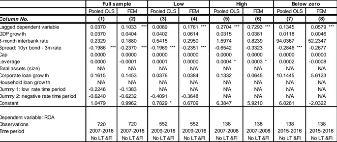
We can observe alternative variations of the model based not on the variable alterations but on the data variation in Table 2 below. As mentioned before we wanted to analyse the result of the test if we trim out the most obvious outliers with regards to the GDP trend observed in our data analysis. Not surprisingly, in such an occasion the redundant fixed effect likelihood ratio test showed that there is no need to include the fixed effect in the regression and a pooled OLS would be sufficient for the analysis. This is because since all the observations followed a similar pattern it could be reasonable to believe that these would have the same intercept and slope thus there was no need for the fixed effect inclusion. However, unfortunately the results of the pooled OLS conveyed that none of the variables were significant at even the 10% significance level.

Table 2. Different model variations (2)

Note. *, ** and *** denote significance at the 0.1, 0.05 and 0.01 respectively. Table made my authors (2018).

The value of the coefficients did not vary a lot in comparison to the main model in column 1. GDP growth was around 0.04 both in the main model and the pooled OLS general GDP trend model, and three months interest rate was around 0.1880 in both. Once again bank book-to-market ratio and leverage remained very low for both models. In the following variables an expressive change in variables was observed where spread in column 1 had a coefficient value of -0.2370 in comparison to -0.1141 in column 3 and corporate loan growth was 0.1453 in comparison to 0.0838 in column 3. Dummy variables also changed quite a lot between the two models with dummy 1 for the low rate period changing in sign where it was -0.1383 it became positive at 0.0638 meaning that from being below by 13% from the high rate interest period following the normal GDP trend in the low period profitability was 6% higher. Yet when the negative interest rate period was analysed, from being below by 62% it was only 37% below when the outliers were not included. If the results were significant, these could be quite reasonable results conveying that if the countries which did not follow the general GDP trend observed in the Eurozone (which were mostly below the norm) are not included in the regression the profitability of the banks is not as strongly affected by the low or negative interest rates.

Column No.

Lagged dependent variable 0.1033 *** 0.0879 ** 0.0438 0.5208 ***

GDP grow th 0.0404 0.0016 0.0356 0.0324

3-month interbank rate 0.1880 0.2082 0.1877 0.2190 ***

Spread: 10yr bond - 3m rate -0.2370 *** -0.1150 -0.1141 -0.3286

Cap 0.0000 0.0000 0.0000 0.0000

Leverage -0.0001 -0.0001 -0.0002 0.0000

Total assets (size) N/A N/A N/A 0.0000

Corporate loan grow th 0.1453 0.1069 0.0838 0.0628

Household loan grow th N/A N/A N/A -0.0133

Dummy 1: low rate time period -0.1383 0.1239 0.0638 N/A

Dummy 2: negative rate time period -0.6232 -0.3560 -0.3714 N/A

Constant 0.9962 0.6372 0.7370 -0.1438

Dependent variable: ROA Observations Time period General GDP trend General GDP trend 1st difference

FEM FEM (not

necessary) No HLG &

Size

Pooled OLS Pooled OLS (4)

720 620 620 648

(1) (2) (3)

2007-2016 2007-2016 2007-2016 2008-2016