EISCAT and Cluster observations in the vicinity of the dynamical polar cap boundary

(1)

http://www.diva-portal.org

This is the published version of a paper published in Annales Geophysicae.

Citation for the original published paper (version of record):

Aikio, A., Pitkänen, T., Fontaine, D., Dandouras, I., Amm, O. et al. (2008)

EISCAT and Cluster observations in the vicinity of the dynamical polar cap boundary.

Annales Geophysicae, 26: 87-105

http://dx.doi.org/10.5194/angeo-26-87-2008

Access to the published version may require subscription.

N.B. When citing this work, cite the original published paper.

Permanent link to this version:

(2)

www.ann-geophys.net/26/87/2008/ © European Geosciences Union 2008

Annales

Geophysicae

EISCAT and Cluster observations in the vicinity of the dynamical

polar cap boundary

A. T. Aikio1, T. Pitk¨anen1, D. Fontaine2, I. Dandouras3, O. Amm4, A. Kozlovsky1,5, A. Vaivdas6, and A. Fazakerley7

1_{Department of Physical Sciences, University of Oulu, P.O. Box 3000, 90014, Finland} 2_{CETP/UVSQ, Velizy, France}

3_{CESR/CNRS, Toulouse, France}

4_{Finnish meteorological Institute, Helsinki, Finland} 5_{Sodankyl¨a Geophysical Observatory, Sodankyl¨a, Finland}

6_{Swedish Institute of Space Physics, Angstr¨omlaboratoriet, Uppsala, Sweden} 7_{Mullard Space Science Laboratory, University College, London, UK}

Received: 16 March 2007 – Revised: 14 December 2007 – Accepted: 20 December 2007 – Published: 4 February 2008

Abstract. The dynamics of the polar cap boundary and auroral oval in the nightside ionosphere are studied during late expansion and recovery of a substorm from the region between Tromsø (66.6◦ cgmLat) and Longyearbyen (75.2◦ cgmLat) on 27 February 2004 by using the coordinated EIS-CAT incoherent scatter radar, MIRACLE magnetometer and Cluster satellite measurements. During the late substorm ex-pansion/early recovery phase, the polar cap boundary (PCB) made zig-zag-type motion with amplitude of 2.5◦ cgmLat and period of about 30 min near magnetic midnight. We sug-gest that the poleward motions of the PCB were produced by bursts of enhanced reconnection at the near-Earth neu-tral line (NENL). The subsequent equatorward motions of the PCB would then represent the recovery of the merging line towards the equilibrium state (Cowley and Lockwood, 1992). The observed bursts of enhanced westward electrojet just equatorward of the polar cap boundary during poleward expansions were produced plausibly by particles accelerated in the vicinity of the neutral line and thus lend evidence to the Cowley-Lockwood paradigm.

During the substorm recovery phase, the footpoints of the Cluster satellites at a geocentric distance of 4.4 RE mapped

in the vicinity of EISCAT measurements. Cluster data in-dicate that outflow of H+and O+ions took place within the plasma sheet boundary layer (PSBL) as noted in some earlier studies as well. We show that in this case the PSBL corre-sponded to a region of enhanced electron temperature in the ionospheric F region. It is suggested that the ion outflow originates from the F region as a result of increased ambipo-lar diffusion. At higher altitudes, the ions could be further

Correspondence to: A. T. Aikio

(anita.aikio@oulu.fi)

energized by waves, which at Cluster altitudes were observed as BBELF (broad band extra low frequency) fluctuations.

The four-satellite configuration of Cluster revealed a sud-den poleward expansion of the PSBL by 2◦_{during ∼5 min.}

The beginning of the poleward motion of the PCB was as-sociated with an intensification of the downward FAC at the boundary. We suggest that the downward FAC sheet at the PCB is the high-altitude counterpart of the Earthward flow-ing FAC produced in the vicinity of the magnetotail neutral line by the Hall effect (Sonnerup, 1979) during a short-lived reconnection pulse.

Keywords. Ionosphere (Auroral ionosphere; Electric fields and currents; Storms and substorms)

1 Introduction

1.1 Polar cap boundary and reconnection

The reconnection between the terrestrial magnetic field lines and the IMF field lines was first discussed by Dungey (1961). During southward IMF, merging of closed geomagnetic field lines with the IMF may take place on the dayside magne-topause at low latitudes. The subsequent tailward transport of open field lines, reconnection at the tail neutral line and sunward convection of closed field lines produce a two-cell convection pattern in the ionosphere. In a steady state picture all the open flux created by dayside reconnection is closed by reconnection at the nightside distant neutral line (DNL) and at any moment the reconnection rates are equal. How-ever, it has been suggested already by Russell (1972) that the dayside and nightside reconnection are separate processes, which may have different rates. Especially during substorms,

(3)

88 A. T. Aikio et al.: EISCAT and Cluster observations near the polar cap boundary sudden reconnection is expected to take place at the

near-Earth neutral line (NENL). This reconnection starts to affect the amount of open flux only when the last closed field line is reconnected.

Siscoe and Huang (1985) modelled unbalanced dayside re-connection by assuming that magnetic flux from the closed field line region enters the polar cap through a restricted part of the circular open-closed boundary (OCB) on the day-side (obviously mapping to the neutral line along the dayday-side magnetopause) and they termed this curved line segment the “merging line” or “merging gap”. When the dayside ing rate was assumed to exceed that of the nightside merg-ing, the polar cap at all local times was increasing in radius. Plasma flow accross the polar cap boundary occured only at the merging gaps, whereas at other local times the OCB moved with the plasma flow. Thus, the OCB outside merg-ing lines was termed “adiaroic”.

Lockwood et al. (1990) and Cowley and Lockwood (1992) discussed the polar cap motion and excitation of flows as a result of solar wind-magnetosphere coupling. They con-sidered the case when merging on the dayside (flux transfer events, FTE) or/and in the nightside (substorm) is a localized and impulsive process. In dayside (nightside) reconnection, the addition (decrease) of flux on the dayside (nightside) cre-ates a two-cell flow pattern, which tends to move the OCB equatorward (poleward) of the previous location. The foci of the convection vortices are displaced from the dawn-to-dusk meridian towards day (night) in the case of dayside (night-side) reconnection.

During northward IMF, merging may happen poleward of the cusps. For pure northward orientation, this merging of open geomagnetic field lines with the IMF generates lobe-cell convection in the magnetosphere and in the ionosphere (Reiff and Burch, 1985). However, when the IMF By

com-ponent is non-zero, closed field lines also reconnect with the IMF on the equatorward side of the cusp and gener-ate merging-cell convection (Nishida et al., 1998; Tanaka, 1999). Open field lines generated by the reconnection on closed field lines convect tailward and subsequently recon-nect in the twisted neutral sheet producing asymmetric merg-ing cells in the ionosphere as shown, for example, by Grocott et al. (2005).

The ionospheric projection of the OCB is the polar cap boundary (PCB). The polar cap boundary determination can be done by using particle boundaries (Newell et al., 1996a,b), optical images (Baker et al., 2000; Brittnacher et al., 1999; Hubert et al., 2006), incoherent scatter (IS) radars (de la Beaujardiere et al., 1991; Blanchard et al., 1995, 1996; Moen et al., 2004; Ostgaard et al., 2005; Aikio et al., 2006) and coherent radars (Chisham et al., 2004; Wild et al., 2004). These methods are discussed in detail in the paper by Aikio et al. (2006) as well as the new IS-radar method that will be utilized in this study. Since it is not based on satellite over-passes, the temporal evolution of the PCB location can be

followed. The advantage of this method is good spatial and temporal resolution.

1.2 Phenomena occurring in the vicinity of the nightside polar cap boundary

The nightside oval has been studied by satellite passes for several decades. Nowadays the plasma environment in the night side oval is typically divided into two main populations, the central plasma sheet (CPS) and the plasma sheet bound-ary layer (PSBL). There is no one commonly accepted way to identify these regions. An early definition comes from East-man et al. (1984): “The plasma sheet boundary layer is a tem-porally variable transition region located between the magne-totail lobes and the central plasma sheet”. Even though much of the oval dynamics is attributed to the PSBL, Newell et al. (1996a,b) note that discrete arcs may lie within the CPS and that CPS is not independent of substorm cycle.

The plasma sheet boundary layer is often occupied by filamentary (Alfv´enic) FACs, intense fluxes of upward and downward electron beams and intense low-energy ion out-flows (e.g. Keiling et al., 2001; Tung et al., 2001). Veloc-ity dispersed ions of type-2, VDIS-2, are typically observed there and they are considered as a signature of quasi-steady reconnection (Sotirelis et al., 1999). The VDIS-2 ion spec-tra show sharp low energy cutoffs, which are smoothly dis-persed in latitude (high energies occurring poleward of low energies).

Ion outflow from the ionosphere to the magnetosphere is a complicated phenomenon, which may be produced by a number of mechanisms. Ion outflows as a function of loca-tion, season, solar and magnetic activity have been studied in several papers (see e.g. Yau and Andre, 1997, and Wilson et al., 2001, 2004, and references therein). Substorm effects on ion outflows have been studied by Wilson et al. (2004), who find that regardless of substorm size, the nightside auroral zone outflow rate increases by about a factor of 2 after onset, reaching its peak level after about 20 min. The PSBL, espe-cially during substorms, is an important source of upflowing ions in the nightside (Tung et al., 2001; Ober et al., 2001).

Magnetic reconnection merging open field lines in the magnetotail affects first plasma within the PSBL. The ef-fect of the Hall term in magnetic reconnection was first pro-posed by Sonnerup (1979), who predicted that the Hall term produces an additional four current loops in the vicinity of the reconnection site. The FACs of this current system are such that in the outermost region near the plasma sheet/tail lobe boundary, field-aligned currents flow out of the mag-netic reconnection site. In the adjacent region, just inside the outflowing current layer, field-aligned currents flow into the magnetic reconnection site. Hence, the FACs of the Hall cur-rent circuit form a thin double-sheet structure near the sepa-ratrix layer. Hall-MHD simulations showed that such small-scale currents can be seen even away from the reconnection site (Yamade et al., 2000).

(4)

Geotail observations in the vicinity of the magnetic recon-nection site of the near-Earth magnetotail during substorm onsets by Nagai et al. (2001, 2003) and Ueno et al. (2002, 2003) have confirmed the existence of the Hall current sys-tem near the PSBL/lobe boundary. Nagai et al. (2001) demonstrated that the counterstreaming electrons in the out-ermost layer are common characteristics of magnetic recon-nection at substorm onsets, and they identified outflowing currents with 6–13 nA m−2 in the outermost layer of the plasma sheet/tail lobe boundary in the immediate vicinity of the magnetic reconnection site. Nagai et al. (1998) sug-gested that the outflowing current is carried by the measured medium energy (near 3 keV) electrons, which stream into the magnetic reconnection site. Recent Cluster observations of the magnetic effect of the Hall currents and the 500–2000 eV electrons flowing towards the reconnection site in the tail at a distance of about −18 RE have given more support to the

Hall-current concept (Asano et al., 2006).

Some evidence that the FACs associated with the Hall cur-rents in the vicinity of the reconnection site would continue to the ionosphere was provided by observations of Ober et al. (2001). They studied an event, where the Polar s/c crossed the PCB near the end of the expansion phase and close to magnetic midnight and found that the boundary was associ-ated with severe east-west plasma flow shears and multiple FACs. At the boundary, Alfv´en waves carried a FAC pair with upward FAC on the equatorward and downward FAC on the poleward side. Yamade et al. (2000) estimated from their simulation that the current densities at the ionospheric level would be 5 µA/m2.

The aim of the paper is to study the dynamics of the polar cap boundary and the oval during one substorm event giving insight into reconnection processes. The polar cap boundary and the poleward part of the oval is studied by using EISCAT VHF radar measurements while MIRACLE magnetometers give information of the distribution of electrojets within the oval. Sections 3 and 4 concentrate on ground-based obser-vations of substorm expansion and early recovery. Cluster pass provides valuable data of plasma environment at an alti-tude of about 21 000 km above the auroral ionosphere during late recovery phase of the substorm. These satellite-ground coordinated measurements are discussed in Sect. 5. Finally, conclusions are given in Sect. 6.

2 Measurements and data analysis

The EISCAT radar experiments used in this paper had the following characteristics. The EISCAT VHF radar, located in Tromsø (TRO, geographic: 69.59◦N, 19.22◦E, cgm: 66.58◦, 102.94◦), was pointed at 30◦elevation with azimuth of 0.5◦ to the west from geographic north. The EISCAT Svalbard Radar (ESR) 42 m antenna in Longyearbyen (LYR, geo-graphic: 78.15◦N, 16.03◦E, cgm: 75.22◦, 111.94◦) is fixed to point in the field-aligned direction and the ESR 32 m

an-70� 80� ₉₀� 100� 110� 120� 130� 140� 150� 85� 80� 75� 70� 65� cgm lon [deg] cgm lat [deg]

C4

C1

VHF

FAST

2052 UT 2056 UT

_TRO

LYR

KIL

BJN

SOR

NAL

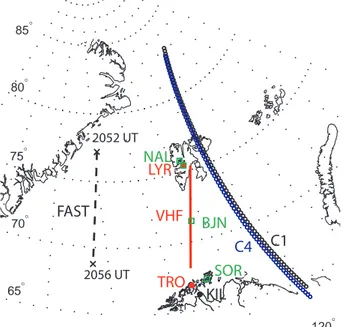
Fig. 1. Cluster orbit for satellites C1 and C4 mapped to the altitude

of 100 km by using the T89c model with Kp=3. The coordinate

system is cgm. The footpoints of C2 and C3 are located between those of C1 and C4. The projection of the EISCAT VHF beam and the mapped FAST orbit are also shown. The sites of the VHF radar (TRO), the ESR radar (LYR) and Kilpisj¨arvi all-sky camera (KIL) are indicated by dots. Squares show the northernmost stations of the MIRACLE magnetometer chain.

tenna was directed at 30◦elevation to azimuth of 0.5◦to the west from geographic north. In this paper, we will not utilize the 32 m data. The VHF and ESR42m beam locations are shown in Fig. 1.

In this study, we estimate the location of the polar cap boundary (PCB) by the EISCAT radar measurements using a method, which is described in detail by Aikio et al. (2006). Electron precipitation in the nightside ionosphere increases the electron temperature Tedue to the collisional heating of

background plasma by the primary and secondary electrons. Since the energy flux of precipitating electrons in the oval is typically higher than that in the polar cap (polar rain precip-itation), electron temperature changes can be used to track the polar cap boundary. When a radar is measuring at a low elevation angle in the north-south direction, the Te profile

along the beam depends both on the horizontal variations in the temperature as well as the height profile of the tem-perature with each measurement point representing different altitude-latitude pair. Typically, Te increases with altitude.

When the PCB is situated between Tromsø and Longyear-byen, the ESR 42 m antenna, measuring in the field-aligned direction, provides the height profile of Tein the polar cap.

(5)

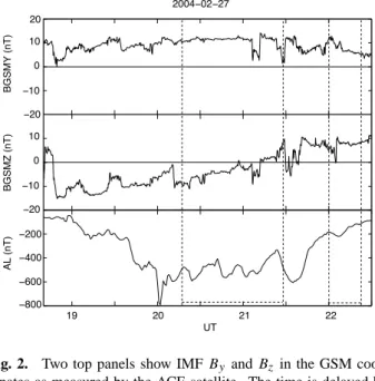
90 A. T. Aikio et al.: EISCAT and Cluster observations near the polar cap boundary AL (nT) 19 20 21 22 UT −20 −10 0 10 20 −20 −10 0 10 −800 −600 −400 −200 2004−02−27 BGSMY (nT) BGSMZ (nT)

Fig. 2. Two top panels show IMF By and Bzin the GSM

coor-dinates as measured by the ACE satellite. The time is delayed by 55 min to account for propagation to the subsolar magnetopause. Bottom panel shows the AL index. The two time intervals marked by vertical lines relate to the PCB fluctuations as observed by EIS-CAT, and the Cluster pass in the PSBL in the end of the recovery phase, respectively.

at corresponding altitudes to get a 1Teprofile. Then, a

pos-itive value of 1Te indicates that electron temperature at that

latitude (and altitude) is enhanced as compared to a corre-sponding altitude in the polar cap. By searching the pole-wardmost latitude where the temperature difference is posi-tive, we get a proxy for the PCB location.

In this paper, we have used two criteria for the PCB search. Method 1 puts the boundary in the polewardmost location where the electron temperature difference plus error stays above zero (as in Aikio et al., 2006) and Method 2 in the location, where the actual electron temperature difference curve crosses zero. If the Te errors are small and the

elec-tron temperature gradient sharp at the boundary, these curves are close to each other.

The temporal resolution of the PCB location is defined by the resolution used in the low-elevation radar data analysis. In this event, a 2-min resolution is used until 21:30 UT, 4-min resolution during 21:30–22:00 UT and 5-4-min resolution 22:00–22:40 UT. The integration time of data was increased as the received signal power decreased to keep the errors at an acceptable level. The range integration in the data anal-ysis resulted in a latitude resolution ranging from 0.18◦ to 0.36◦cgmLat, higher resolutions corresponding to lower lat-itudes.

The equivalent east-west currents in the ionosphere were calculated from the magnetic X components of a north-south chain of MIRACLE magnetometer stations by using 1-D-upward field continuation method (Vanham¨aki et al., 2003).

The northernmost of the stations (NAL, LYR, BJN and SOR) used are shown in Fig. 1.

The Cluster orbit during the studied event is explained in Sect. 5.1. We have utilised measurements from four Cluster instruments: the Electric Field and Wave Instrument, EFW (Gustafsson et al., 1997), the Fluxgate Magnetometer, FGM (Balogh et al., 1997), the Plasma Electron And Current Ex-periment, PEACE (Johnstone et al., 1997) and the Cluster Ion Spectrometry, CIS (R´eme et al., 2001).

The EFW experiment consists of two pairs of spherical probes deployed in the spin plane to measure the electric field. The component of the electric field along the spin axis is not measured. To study the electric field fluctuations, we use high time resolution, 40 ms. These data are presented in the DSI (despuned inverse) coordinate system, which is very close to GSE. In DSI the x-axis is in satellite spin plane as close as possible to the x-axis in GSE, the z-axis is along the satellite spin axis with the inversed sign of spin vector be-cause then it is as close as possible to there z-axis in GSE, and y-axis closes the right-handed coordinate system.

Data from the FGM instrument is used to calculate the field-aligned current densities for each s/c separately. The contribution of the Earth’s average geomagnetic field is sub-tracted from the spin-resolution (4 s) measurement and the remaining variations are fitted to the magnetic field of an in-finite current sheets.

The HEEA (High-Energy Electron Analyser) sensor of the PEACE instrument is used. It covers the energy range from 36.2 eV to 23.7 keV. The full 4π solid angle coverage is com-posed of a grid of 12 polar bins by 32 azimuthal bins; each bin is 15◦_{by 11.25}◦_{. The data are acquired simultaneously}

in all 12 polar bins while the azimuthal data are gathered as the satellite spins.

The CIS experiment consists of two distinct instruments measuring complete 3-D ion distributions: the CIS-1/CODIF spectrometer which separates the major ion species (H+, He++, He+, and O+), with energies up to 40 keV/e and the CIS-2/HIA analyser which gives the ion distributions (with-out mass resolution) from 5 eV/e to 32 keV/e.

3 IMF and mainland optical observations

The IMF was measured by the ACE satellite at

XGSM∼218 RE. During the studied time interval, the

solar wind speed stayed rather steady, at about 410 km/s, which resulted in a time delay of about 55 min to the dayside subsolar magnetopause at about 10 RE. In the following

discussion, we use these delayed times. The dynamic pressure of the solar wind remained small (2–3.5 nPa) throughout the time interval. After being several hours in the northward direction, the IMF Bz decreased abruptly from

5 nT to −15 nT at about 18:45 UT (Fig. 2). For the next two hours, the IMF Bz varied between −15 and −5 nT and By

(6)

but was again negative for a short time interval during 21:30–21:40 UT, after which the IMF remained northward (value about 10 nT) until the end of the studied time interval, 22:40 UT with an exception of a short-lived decrease of Bz

to zero at 22:08 UT.

The optical observations were made on the mainland by the Kilpisj¨arvi (KIL, geographic: 69.02◦N 20.79◦E; cgm: 65.76◦ 104.49◦) all-sky camera (see Fig. 1). The cam-era showed a very faint auroral arc drifting southward at 19:00 UT, which is a typical feature during a growth phase of a substorm (data not shown). In spite of an onset of Pi2 pulsations at about 19:20 UT at mid-latitude magne-tometers (NUR, UPS, HAD), the activated arcs continued to drift equatorward. At 19:41 UT a westward travelling surge (WTS) appeared from the east and produced poleward ex-pansion of auroras in the studied MLT zone. So, obviously the substorm onset time was within the 19:20–19:40 UT time interval and the onset location was to the east of KIL. The AL index in Fig. 2 shows also a rapid decrease starting at about 19:40 UT.

The WTS stayed in the field-of-view (f-o-v) of the KIL all-sky camera (ASC) until 20:08 UT. After that, the WTS moved towards west and the auroral bulge was left hind. The bulge expanded poleward and disappeared be-yond the KIL ASC f-o-v (70◦cgmLat in the northern direc-tion) at 20:08 UT. The AL index shows a sharp minimum at 20:02 UT (Fig. 2), but the equivalent currents of the west-ward electrojet (WEJ) integrated along the whole north-south chain of the MIRACLE magnetometers reach their maximum only at 20:20 UT (curve not shown, but look at Fig. 5). Tra-ditionally, the time of the AL minimum (WEJ maximum) would mark the end of the expansion phase and beginning of the recovery phase (e.g. McPherron, 1995). However, the magnitude of the AL index stays high until 21:40 UT and a rapid recovery starts only after that.

In this paper, we concentrate on the time interval af-ter 20:00 UT, which covers the late expansion and recovery phases of the substorm. From this time period we have no optical observations from the region of interest.

4 EISCAT radar and ground magnetic observations 4.1 PCB and F-region electron and ion temperatures Figure 3 shows the Teof the VHF radar in the time-latitude

coordinate system and the black curve is the PCB determined by using this data together with the ESR field-aligned Tedata

(Method 1). The figure shows that the electron temperature is increased at all latitudes equatorward of the PCB down to 69.6◦, which is the lowest latitude provided by the method (corresponding to a height of 200 km).

Ion temperatures shown in Fig. 4 behave differently. They are increased within a relatively narrow zone in the vicinity of the PCB, and only during a part of the observing time.

Lockwood and Fuller-Rowell (1987a, b) and Lockwood et al. (1988) introduced the idea that a band of high Ti might

form on the equatorward (poleward) side of a contracting (expanding) polar cap near dawn and dusk so that the en-hanced Tiwould always be located on the trailing side of the

boundary. The explanation required two things. First, ini-tially an equilibrium state had been reached where the ther-mospheric winds and ion flows had adapted to each other. Then, a sharp boundary of ion flows would move rapidly in horizontal direction producing ion frictional heating at loca-tions where ion flows had turned into opposite direction than the winds. Experimental evidence of this effect were pro-vided by Lockwood et al. (1988) showing observations of the motion of a sharp flow reversal boundary in the dawn sector and by Davies et al. (2002) using data from the pre-noon sec-tor. However, Moen et al. (2004) noted that the trailing edge concept of enhanced Ti by Lockwood et al. was not

consis-tent with their observations made near noon. They observed a band of high Tiwhich persisted for 8 h and zig-zagged

north-south. This band of high Ti could locate on the equatorward

side of the flow reversal boundary as it was moving equa-torward, on both sides of the flow reversal boundary, and at times it was not related to the flow reversal boundary at all. In addition, the band of high dayside Ti was located on open

field lines, but its equatorward edge was not a good proxy for the OCB.

In this nightside event, the poleward edge of the high Ti

band follows quite well the PCB determined by the pole-ward edge of high Teuntil 21:14 UT. Data from the coherent

HF radars of the Super Dual Auroral Radar Network (Su-perDARN, Greenwald et al., 1995) (not shown) reveal that before 19:30 UT a two-cell convection pattern prevails, with the VHF radar measuring the south-westward plasma flow in the evening convection cell. There has been enough time for the neutral wind to adapt itself to the 2-cell pattern. The substorm onset is followed by the arrival of the WTS to the longitude of EISCAT during 19:41–20:08 UT. The auroral bulge behind the head of the WTS expands poleward, carry-ing along eastward plasma flows (westward current, see also Fig. 5). When these eastward plasma flows meet the assumed westward winds, increased ion frictional heating is expected on the equatorward side of the poleward expanding boundary according to the trailing edge concept. This is exactly what is seen during 20:10–20:26 UT (period A) and also 20:42– 20:58 UT (period C).

Since the PCB spends only a relatively short time interval at higher latitudes, the neutral winds are not expected to be affected much by the ion drag and the trailing edge concept may not work during an equatorward recovery of the PCB. Indeed, during 20:26–20:42 UT (period B), the band of in-creased Ti is very wide and even though some part of it is on

the poleward side of the PCB, the main part of it is equator-ward of the boundary. During 20:58–21:12 UT (period D),

Ti is clearly less enhanced and coincides with the PCB.

(7)

92 A. T. Aikio et al.: EISCAT and Cluster observations near the polar cap boundary

Aacgm latitude [deg]

Electron temperature 27 Feb 2004

Time [UT] Tromsö VHF Az=359.45 El=30

20:00 21:00 22:00 68 69 70 71 72 73 74 75 1 1.5 2 0 500 1000 1500 2000 2500 3000 3500 Te [K ]

Electron temperature 27 Feb 2004

Fig. 3. Electron temperature measured by the VHF radar. The black curve is the PCB based on this data and the ESR field-aligned Te

measurement. Cluster C1 (black) and C4 (blue) orbits are marked by triangles at locations of ion outflow.

Aacgm latitude [deg]

Ion temperature 27 Feb 2004

Time [UT] Tromsö VHF Az=359.45 El=30

20:00 21:00 22:00 68 69 70 71 72 73 74 75 1 1.5 2 0 500 1000 1500 2000 2500 3000 3500 Ti [K ]

Ion temperature 27 Feb 2004

A

B

C

D

E

Fig. 4. Ion temperature measured by the VHF radar in the same format as Fig. 3. Time intervals denoted by A to E are shown in the lower

part of the figure.

disappears entirely and is not visible during period E (the poleward motion of the PCB). Since the Ti enhancement is

proportional to (vi−vn)2, obviously the velocity difference between ions and neutrals has become small.

4.2 Equivalent currents and the PCB

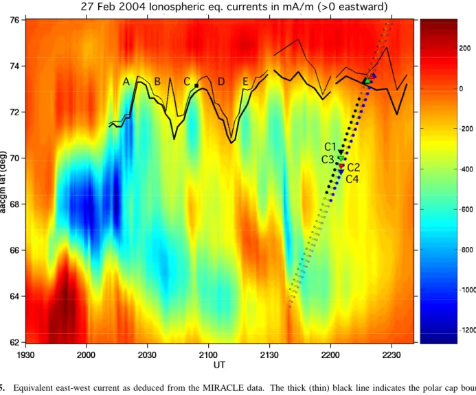
The equivalent east-west currents are shown in Fig. 5. Af-ter 19:30 UT, a westward current region drifting southward

(8)

27 Feb 2004 Ionospheric eq. currents in mA/m (>0 eastward) A B C D E C1 C2 C3 C4

Fig. 5. Equivalent east-west current as deduced from the MIRACLE data. The thick (thin) black line indicates the polar cap boundary from the EISCAT VHF radar by using Method 1 (Method 2). The dotted lines are mapped Cluster s/c C1–C4 locations and the filled circles indicate positions where C1 and C4 observe ion outflow. The triangles with tip down are the locations of the s/c at 21:05 UT. The orbits of the satellites in latitude and longitude are shown in Fig. 1. The triangles with tip up are the locations of the PCB by each s/c (see text). The black square shows the PCB location from FAST data. Letters from A to E are same time intervals as in Fig. 4.

becomes visible. It is obviously associated with the activated aurora, also drifting equatorward. The steplike poleward ex-pansion and intensification of the westward electrojet (WEJ) at 19:45 UT, is due to intrusion of the WTS to the magne-tometer meridian from the east, as shown by the KIL all-sky camera. The poleward edge of the substorm current wedge (SCW) stays at about a constant latitude (about 70◦ cgm-Lat) until 20:08 UT, after which a poleward expansion oc-curs. At the same time, a significant equatorward expansion of the SCW currents occurs, which results in a very wide oval, about 10◦in cgmLat.

The PCB can be estimated by the EISCAT radar method after 20:08 UT and then the PCB traces rather closely the poleward edge of the WEJ. An exception occurs in the very beginning (20:08–20:24 UT) of the time interval, when the intense WEJ seems to extend to the poleward side of the PCB. This may not be a real effect, but related to the sparsely

located magnetometers within this region combined with bursts of intense currents.

The WEJ has three short-lived intensifications close to the PCB, which are associated with a simultaneous poleward ex-pansion of the PCB. These start at 20:18 (period A), 20:49 (period C) and 21:15 UT (period E), i.e. they are separated by 25–30 min. These rather short-lived (duration about 10 min) intesifications of the WEJ are restricted to latitudes poleward of approximately 70◦cgmLat.

Each expansion is followed by contraction, so that the result is a periodic oscillatory motion (zig-zag-type) of the PCB with an amplitude of about 2.5◦. Alltogether 2.5 oscil-lations occur. When the last oscillation has reached its max-imum at about 21:25 UT, the PCB doesn’t return to a lower latitude, but stays in the north. At that time the IMF has be-come northward.

(9)

94 A. T. Aikio et al.: EISCAT and Cluster observations near the polar cap boundary During period C, the FAST satellite passes from north to

south about 1.5 h earlier in MLT time (see Fig. 1). The FAST ions show the VDIS-2 signature and the polar rain electrons a velocity dependent cutoff (data not shown) indicating ongo-ing reconnection. For a polar cap boundary, we selected a lo-cation where high-energy (25 keV) ions appear and electron energy fluxes start to increase (20:54:00 UT). The mapped cgm latitude of the boundary is marked by a solid square in Fig. 5 and it is very close to the PCB location at the EISCAT longitude.

4.3 Origin of PCB fluctuations

During late substorm expansion, the polar cap boundary ex-hibits a zig-zag-type motion between about 70.5◦ and 73◦ cgmLat with a period of 25–30 min. The PCB motions can be explained by at least by three different mechanisms: (1) Large-scale spatial structures drifting in the east-west direc-tion along the boundary, (2) Global oscillatory modirec-tions of the magnetosphere, and (3) Variations in flux reconnection rates. We will discuss these options below.

The poleward boundary of oval may sometimes host dif-ferent wavelike structures or regions of enhanced luminosity, which can travel along the boundary (see e.g. Elphinstone et al., 1995). Since no global images of the auroral oval are available, we can’t make the distinction (the KIL all-sky camera doesn’t see far enough north). However, the oscilla-tions observed are quite large in amplitude, 2.5◦in latitude and hence, if spatial features, they are very large in size.

Lyons et al. (2002) suggested that global mode Ps6 fre-quency oscillations could play a role in polar boundary inten-sification (PBI) events. Those events occur at the poleward boundary of the oval and the typical period is 10 min, but sometimes 25–30 min periods are seen. Lyons et al. (2002) proposed that the PBI events would be manifestations of a global oscillatory mode of the magnetosphere. Those global ULF waves would modulate particle transport and magnetic fields in the whole nightside magnetosphere.

Global magnetospheric MHD cavity and/or waveguide modes are generally attributed to frequencies higher than 1 mHz (periods shorter than 15 min). For excitation of cavity modes, a pressure pulse or a sudden change in IMF could act as a trigger. Indeed, Ostgaard et al. (2005) found oscillations of the nightside PCB at periods of 10–15 min.

Also sub-mHz oscillations have been found from the mag-netosphere, especially at 0.5 mHz (30 min period) (Kepko et al., 2002; Kepko and Spence, 2003). It has been suggested that at sub-mHz frequencies, the magnetosphere could be a passive oscillator, driven by external periodic forcing by the solar wind.

In this event, the period of the PCB oscillations is 25– 30 min. However, none of the magnetometer data we have checked (the MIRACLE magnetometers, the INTERMAG-NET mid/low latitude magnetometers, and the GOES 10 and 12 magnetometers at the geostationary orbit on the dayside)

show any evidence of global ULF waves. Therefore we rule out this mechanism.

The third mechanism is provided by variations in the re-connection rates between the terrestrial magnetic field lines and the IMF field lines. This issue is discussed in Introduc-tion. The balance between the dayside and nightside recon-nection determines the location of the PCB. If a nightside re-connection pulse (relatively short-lived period of increased reconnection rate) takes place, the localized region of in-creased closed flux is pushing the PCB poleward within that region. After the pulse has decayed, the polar cap boundary is relaxing to equilibrium position at all local times.

In this event, we observe three clear poleward expansions and two first of them are also associated with recoveries. In addition, Fig. 5 shows that poleward expansions during pe-riods A, C and E are associated with an enhanced WEJ in the vicinity of the boundary. We suggest that the cause is en-hanced precipitation, which obviously originates from field-lines Earthward, but rather close to the neutral line. These en-hancements remain local and don’t extend to the main oval, so obviously there is no large-scale effect on the magnetotail. We also checked geostationary particle data from the LANL satellites (data not shown) and noted that these periods are not associated with particle injections to the geostationary orbit unlike the substorm onset before 20:00 UT.

Since the EISCAT experiment mode used in this measure-ment didn’t allow determination of the 2-D plasma velocity and boundary orientation, we were not able to calculate the ionospheric reconnection rates. However, since the poleward expansions of the PCB are associated with enhanced elec-trojets and hence plausibly of particle precipitation in the vicinity of the boundary, and since FAST data suggest that the boundary motion occurs at least within a region 1.5 MLT wide, we favour option 3 (reconnection pulses) as the expla-nation of these fluctuations.

There are some observations of the typical time scales as-sociated with PCB motions. On the dayside, Lockwood et al. (2005) reported motions of the entire dayside PCB both poleward and equatorward during different substorm phases. Those motions occurred on time scale of hour(s). In addition to that pulsing on time scales of 2–20 min during southward IMF was observed. As mentioned earlier in this section, Ost-gaard et al. (2005) found oscillations of the nightside PCB at periods of 10–15 min. In the very beginning of substorm expansion, poleward expansion has been observed to occur in the form of individual bursts, which are separated by 2– 10 min (Aikio et al., 2006). One could also note that bursty bulk flow (BBF) events in the central plasma sheet organize themselves in 10-min time scale flow enhancements (Naka-mura et al., 2005). It is believed that fast flows are due to acceleration in the reconnection region. The 30 min period observed in this study is longer than the time scales quoted above, but with the same order of magnitude.

(10)

PSBL PCB Polar rain

C1 PEACE HSPAD Day ; 27/2/2004 Y(eV) - Z(ergs/(cm**2–str–s–eV))

Fig. 6. PEACE measurement on C1 of electron energy fluxes in units of erg cm−2sr−1s−1eV−1in the upward (top), perpendicular (middle) and downward (bottom) directions. The PSBL and Polar rain regions are shown.

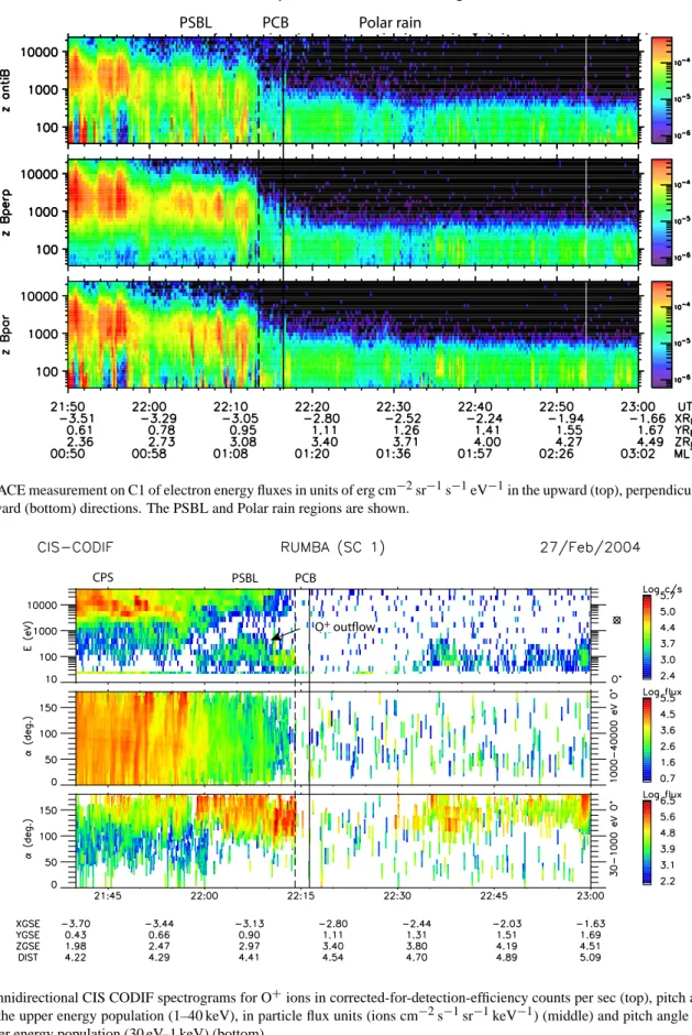
CPS PSBL PCB

O+_outflow

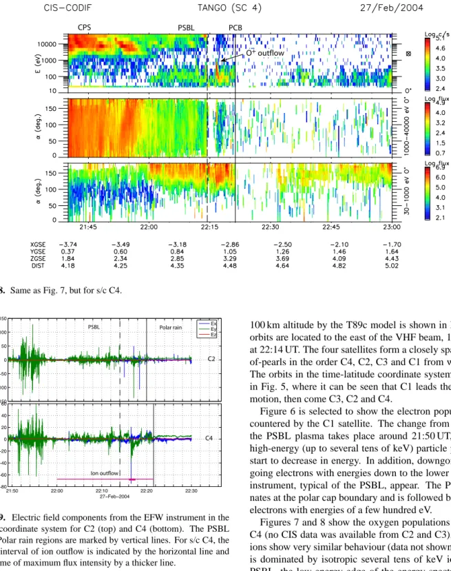
Fig. 7. Omnidirectional CIS CODIF spectrograms for O+ions in corrected-for-detection-efficiency counts per sec (top), pitch angle distri-bution for the upper energy population (1–40 keV), in particle flux units (ions cm−2s−1sr−1keV−1) (middle) and pitch angle distribution for the lower energy population (30 eV–1 keV) (bottom).

(11)

CPS PSBL PCB

O+_outflow

Fig. 8. Same as Fig. 7, but for s/c C4.

−150 −100 −50 0 50 100 150 E [mV/m] DSI~GSE sc2

Full time resolution electric field. Not calibrated.

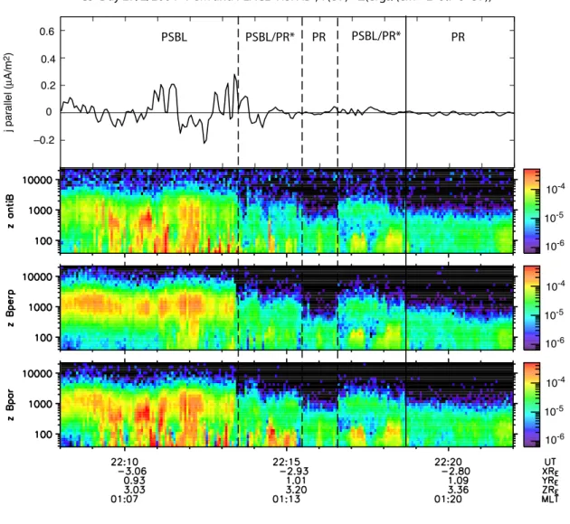
21:50 22:00 22:10 22:20 22:30 −80 −60 −40 −20 0 20 40 60 E [mV/m] DSI~GSE sc4 27−Feb−2004 Ex Ey Ez PSBL Polar rain Ion outflow C2 C4

Fig. 9. Electric field components from the EFW instrument in the

DSI coordinate system for C2 (top) and C4 (bottom). The PSBL and Polar rain regions are marked by vertical lines. For s/c C4, the time interval of ion outflow is indicated by the horizontal line and the time of maximum flux intensity by a thicker line.

5 Cluster observations during substorm recovery 5.1 Magnetospheric regions traversed and ion outflow The four Cluster satellites were on the perigee pass over the Northern Hemisphere during the substorm recovery phase. The Cluster orbit mapped along magnetic field lines to a

100 km altitude by the T89c model is shown in Fig. 1. The orbits are located to the east of the VHF beam, 10◦cgmLon at 22:14 UT. The four satellites form a closely spaced string-of-pearls in the order C4, C2, C3 and C1 from west to east. The orbits in the time-latitude coordinate system are shown in Fig. 5, where it can be seen that C1 leads the northward motion, then come C3, C2 and C4.

Figure 6 is selected to show the electron populations en-countered by the C1 satellite. The change from the CPS to the PSBL plasma takes place around 21:50 UT, where the high-energy (up to several tens of keV) particle populations start to decrease in energy. In addition, downgoing and up-going electrons with energies down to the lower limit of the instrument, typical of the PSBL, appear. The PSBL termi-nates at the polar cap boundary and is followed by polar rain electrons with energies of a few hundred eV.

Figures 7 and 8 show the oxygen populations for C1 and C4 (no CIS data was available from C2 and C3). Hydrogen ions show very similar behaviour (data not shown). The CPS is dominated by isotropic several tens of keV ions. In the PSBL, the low-energy edge of the energy spectrum for the high energy population increases with latitude, which is a characteristic signature of velocity-dispersed ions of type 2. The VDIS-2 signature is interpreted to be produced by re-connection in the magnetotail: the highest energy ions arrive poleward of the lower energy ions, which spend a longer time when traveling from the reconnection site to the ionosphere and thus suffer from a greater inward drift.

(12)

C1 Day 27/2/2004 FGM and PEACE HSPAD ; Y(eV) - Z(ergs/(cm**2–str–s–eV)) 10-4 10-5 10-6 10-4 10-5 10-6 10-4 10-5 10-6 j parallel ( µA/m 2) –0.2 0 0.2 0.4 0.6 _PSBL _PSBL/PR* _PR

Fig. 10. Downward FAC for C1 (top panel) and PEACE data in the same format as Fig. 6 (bottom panels).

Both satellites show upflowing (see the bottom panel for pitch-angle of low-energy ions) O+and H+ions within the PSBL region with energies of 50–500 eV. Hydrogen fluxes exceed 107cm−2s−1 while oxygen fluxes are somewhat smaller. This region of ion outflow is marked by filled dots in Fig. 5. One can see that this 4◦cgmLat (6◦cgmLat) wide region by C1 (C4) corresponds to the poleward part of the oval and the poleward part of the westward electrojet region up to the PCB. In Figs. 3 and 4 the ion outflow region is shown by triangles. Ion outflow coincides with a region of enhanced electron temperature rather than increased ion perature in the ionospheric F region. Elevated electron tem-perature increases the scale height of ions and the ambipolar diffusion coefficient. For example, the measured ion tem-perature of 2500 K (at an altitude 400 km) corresponds to a thermal energy of 0.3 eV for ions. If the observed ions are of ionospheric origin, they must be energized between the ionosphere and the Cluster altitude (3.4 RE). One possibility

is energization by waves.

Figure 9 shows the full resolution (40 ms, correspond-ing frequencies up to 12.5 Hz) electric fields measured by satellites C2 and C4 (no data was available from C1 and C3). Two bursts of intense fluctuations can be seen. The most in-tense flux of upflowing ions measured by C4 occurs at about 22:17 UT and at the same time enhancement in the ampli-tude of electric field fluctuations are seen. These fluctuations belong to the family of broad band electrostatic extra low frequency (BBELF) waves which extend from DC to several hundred Hz. At least some of the wave modes classified as BBELF can heat the ions (Andr´e et al., 1998; Lynch et al., 2002). The heated ions are then pushed upward along mag-netic field lines by the mirror force. The region of BBELF waves may extend well below the Cluster altitudes.

(13)

C3 Day 27/2/2004 FGM and PEACE HSPAD ; Y(eV) - Z(ergs/(cm**2–str–s–eV)) PSBL 10-4 10-5 10-6 10-4 10-5 10-6 10-4 10-5 10-6 j parallel ( µA/m 2) –0.2 0 0.2 0.4 0.6 _PSBL/PR* _PR _PSBL/PR* _PR

5.2 Cluster measurements of electrons and field-aligned currents

Comparison of the PEACE electron data and the calculated FACs for all four Cluster satellites from the poleward part of the PSBL and beginning of the polar rain region are shown in Figs. 10–13. We first turn attention to the electron data to determine the location of the PCB.

At the polar cap boundary, the energetic electron fluxes drop off and polar rain begins. However, even in a stationary situation the boundary may be somewhat ambiguous, since field lines are convecting earthward after reconnecting at the neutral line and only electrons with infinite speed would trace the neutral line to the ionosphere. Determining which elec-trons are polar rain elecelec-trons on open field lines is also am-biguous because the energy of polar rain electrons varies from event to event. In this case, it seems that polar rain elec-trons occur at energies below 1 keV (see also Fig. 6) and we

use this definition to characterize polar rain (PR) electrons in Figs. 10–13. The location where the PR electrons are en-countered is marked by a solid line. However, intense fluxes of a few keV electrons drop off at a lower latitude and de-fine another boundary for C1, which is marked by a dashed line (Fig. 10). Equatorward of this boundary, the electron population is characteristic of the PSBL. Between these two boundaries, electron fluxes at C1 are structured and weak, but extend somewhat above the 1-keV limit. We have marked this region by PSBL/PR?, since it has characteristics of both regions.

The satellite to follow C1 on the poleward orbit is C3. The unstructured polar rain is observed continuously on the poleward side of the last solid line and the PSBL is located equatorward of the first dashed line in Fig. 11. Inside the PSBL/PR?region, fluxes have increased from that of C1 and in the middle of this region there is a short interval when electrons are typical of polar rain.

(14)

10-4 10-5 10-6 10-4 10-5 10-6 10-4 10-5 10-6

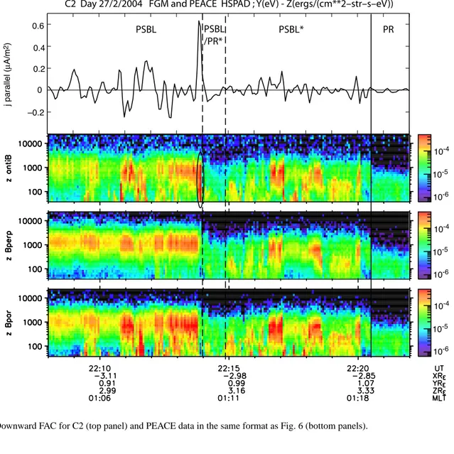
C2 Day 27/2/2004 FGM and PEACE HSPAD ; Y(eV) - Z(ergs/(cm**2–str–s–eV))

j parallel ( µA/m 2) –0.2 0 0.2 0.4 0.6 _PSBL _PSBL _PSBL* _PR /PR*

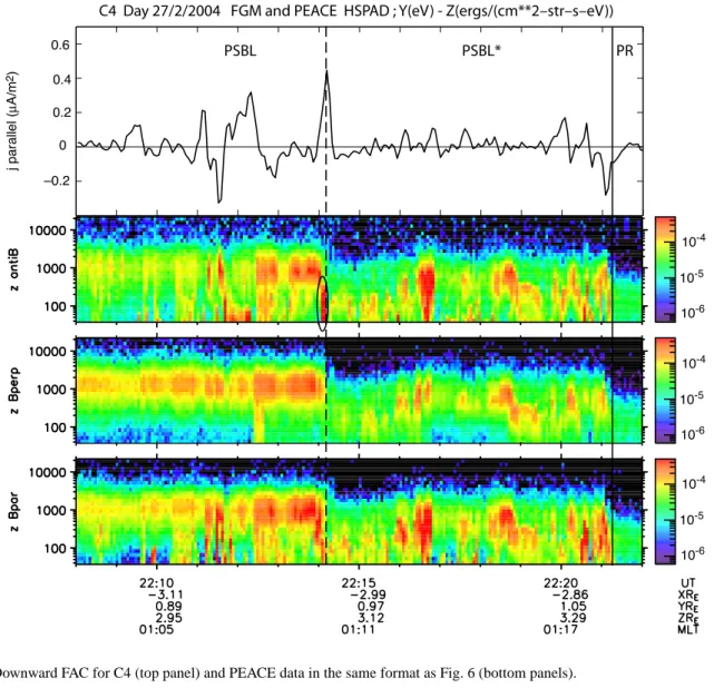
C2 follows C3 and and for a short period of time C2 is embedded in a region of low-energy weak fluxes, marked as PSBL/PR?in Fig. 12. After that, a pronounced enhancement of electron fluxes is observed by C2. For C4 the increase of fluxes is observed almost immediately poleward of the dashed line (Fig. 13).

We argue that the PSBL has suddenly expanded poleward and this expanded region we denote by PSBL?_.

The top panels of Figs. 10 to 13 show the FACs. The field-aligned current densities have been calculated by assuming that they are stationary sheet currents aligned perpendicular to s/c orbit (sheet alignment in the east-west direction). The values shown are at the satellite altitude and to get the values in the ionosphere they must be multiplied by about 100 due to the decrease of the flux tube cross-sectional area towards the ionosphere.

Alternating upward and downward currents are seen in the PSBL by all four s/c. When averaged over the PSBL, a net

downward FAC is obtained, which is in accordance with the Region 1 current direction in the post-midnight sector. Ear-lier observations of magnetospheric FACs in the PSBL have also been in accordance with the Region 1 current directions (e.g. Ohtani et al., 1988).

Satellites C1 and C3 measure a similar broad (width about 0.4◦in latitude) fluctuating FAC region with preference of downward FAC and intensity up to 0.2 µA/m2in the vicin-ity of the poleward edge of the PSBL. Satellites C2 and C4 cross this boundary 30–60 s later and they observe that the downward FAC structure just at the boundary has intensified and become narrower. The FAC density is 0.6 µA/m2at C2 and 0.4 µA/m2at C4. For all s/c, the downward FAC region extends on both sides of the boundary and upward FAC re-gions of clearly smaller intensities are observed on both sides of the downward FAC.

The current carriers of the intense downward FAC are up-going electrons of broad energy range up to 2 keV at C2

(15)

100 A. T. Aikio et al.: EISCAT and Cluster observations near the polar cap boundary 10-4 10-5 10-6 10-4 10-5 10-6 10-4 10-5 10-6 j parallel ( µA/m 2) –0.2 0 0.2 0.4 0.6

C4 Day 27/2/2004 FGM and PEACE HSPAD ; Y(eV) - Z(ergs/(cm**2–str–s–eV)) PR PSBL*

PSBL

(22:13:52 UT) and up to 400 eV at C4 (22:14:12 UT), as seen in the second panel of Figs. 12 and 13 (feature is encir-cled). As discussed by Aikio et al. (2004), these are probably electrons of ionospheric origin, which have been accelerated below the satellite. There seems to be a positive correlation between the FAC density and the maximum energy of the upflowing electrons.

5.3 Interpretation of Cluster observations in terms of a tem-poral change

We turn our attention again to Figs. 7 and 8, where the time instants corresponding to the first vertical line (first exit from the PSBL) and the last vertical line (final exit to polar rain) from Figs. 10 and 13 are added. At C1, no ions are observed poleward of the PSBL. At C4, higher energy ions disappear at the time of the first exit from the PSBL and then after a few minutes fluxes recover at lower intensity. Hydrogen ions

(data not shown) show a similar gap and the recovered fluxes are more intense than those of O+_{shown, but smaller than in}

the original PSBL. These H+fluxes also extend to the loca-tion of the final PCB.

The low-energy O+_{population at C4 which is flowing}

up-ward from the ionospheric direction, doesn’t show a similar gap, but maximum fluxes and energies are encountered at the point where the high-energy ion population recovers. The poleward boundary of upflowing ions extend to the location of the new PCB.

To clarify the event in terms of spatial and temporal evolu-tion, we show the downward FAC by all the four s/c as a func-tion of time and corrected geomagnetic latitude in Fig. 14. The FAC intensity is color coded with yellow and red col-ors corresponding to downward FAC, blue color to upward FAC and green color to no FAC. (The interpolation used in plotting the s/c data causes some artificial structuring in the currents so that typically the current sheets seem to contain

(16)

four fluctuations). The data from satellites show a consis-tent picture: several FAC structures drifting southward are seen by all the satellites, e.g. around 22:06, 22:09, 22:11 and 22:13 UT. The FACs tend to occur in pairs with upward FACs equatorward of the downward FACs, which is a typical signature of morningside arcs (Aikio et al., 1993). The slope of the structures remains about the same and corresponds to drift speed of about 1 km/s equatorward. So, the FAC struc-tures are likely to be associated with auroras drifting equa-torward in the poleward part of the auroral bulge. The drift speed is rather high, but the line-of-sight measurements from the Iceland East SuperDARN radar (data not shown) reveal similar plasma convection velocities during this time interval slightly north of Cluster footpoints.

The ionospheric current density at the original PCB can be get by multiplying the FAC density estimate based on an as-sumption of a stationary current sheet at Cluster altitude by a factor of 100·0.3=30, where 100 comes from the geometry of the flux tubes and 0.3 from the motion of the current sheet towards the poleward moving satellites.The equatorward ve-locity of the current sheet can be deduced from Fig. 14 and it is about 1000 m/s, whereas the mapped satellite velocity in the poleward direction is 460 m/s. By inserting them in equation vsat/(vsat+vfac)(e.g. Aikio et al., 2004), we get a correction factor 0.3. Thus 0.2 µA/m2and 0.6 µA/m2at C1 and C4, respectively, correspond to 6 and 18 µA/m2at the ionospheric level.

A clear change in the drift pattern of Fig. 14 occurs close to 22:15 UT. The equatorward drift has stopped and rather poleward moving structures can be seen. The plus-marks de-note the exit from the PSBL and it is dede-noted by “original PCB”. The final crossing to the polar cap is marked by stars and it is denoted as “final PCB”.

In Fig. 15 only the perpendicular electron fluxes are se-lected from each s/c and they are stacked so that the common horizontal axis is the geomagnetic latitude. The string-of-pearls configuration during the studied time interval was such that the satellites were at a given latitude with 1-min sepa-ration. The two red lines show how a simultaneous event at all satellites would look like in the figure. The white dashed line shows the location of the “original PCB”, which is drifting equatorward with the plasma (slope is larger than that of the red line which also corresponds to poleward mo-tion at the same velocity as the satellites). At about 22:15 UT a change from equatorward drifting structures to poleward moving structures takes place, in accordance with FAC drifts in Fig. 14. The three black lines show structures which are moving poleward with a velocity that is slightly faster than the mapped satellite velocity in the poleward direction (the slopes of black lines are somewhat smaller than that of the red line). The identified structures are first observed by C4, then C2 and they seem to extend even to C3 producing there weak fluxes of electrons above 1 keV. Enhancement of low-energy fluxes at C1 occurs also in connection with this poleward expansion. The poleward expansion stops at about

C1 C4 C3 C2 70 71 72 73 74 75 aacgmLat (deg) −0.2 −0.1 0 0.1 0.2 µA/m2 Jdown 2004−02−27 time 22 UT + min 4 6 8 10 12 14 16 18 20 22 24 original PCB final PCB

Fig. 14. Downward FAC in time-latitude coordinates. The FAC magnitude is color coded and data from all four satellites is used.

22:19–22:20 UT and the final PCB latitude (solid white line) becomes as 73.6◦.

To summarise the observations we note the following. All the poleward moving Cluster satellites cross a spatial bound-ary between 22:13–22:14 UT. After the crossing, polar rain type electrons are observed by all the other satellites but the last (C4). The most poleward satellite, C1, continues to see electrons of polar rain energies after that and ions disappear. For other satellites, the electron fluxes recover again and after a pause, high-energy ions reappear at C4. The drift patterns identified from FACs and electron structures indicate that around 22:15 UT a poleward expansion of the PSBL plasma occurs. The velocity of the poleward expanding boundary is only a little faster than the satellite velocity in the poleward direction, so that the boundary catches C2 and to some ex-tent C3, but not properly C1. The duration of the poleward expansion is order of 5 min. We suggest that we have ob-served a short-lived and possibly spatially localized recon-nection burst at the nightside neutral line during substorm recovery.

The interesting observation is the downward FAC at the original PCB, just when it was about to start expanding poleward. The theoretical model of the Hall current system in the vicinity of the neutral line predicts field-aligned cur-rent out of the reconnection site. To our knowledge, there has not been conclusive evidence that this field-aligned cur-rent component would continue to the ionosphere. However, the data by Ober et al. (2001) and the data presented above, suggest this might be the case. Simultaneous and conju-gate observations in the ionosphere and in the mid-tail would be needed to conclusively confirm this hypothesis. In this study, we find that the downward FAC is carried by anti-parallel moving electrons of energies up to 2 keV, which is

(17)

102 A. T. Aikio et al.: EISCAT and Cluster observations near the polar cap boundary 72o ₇₃o 71o ₇₄o aacgm Lat C1 to C3 to+ 1 min C2 to+ 2 min C4 to+ 3 min

Fig. 15. Perpendicular electron fluxes from C1 (top panel), C3, C2 and C4 (bottom panel) presented as a function of geomagnetic latitude.

The time interval covered by each of the satellites is 22:08–22:22 UT. The white dashed line shows the drift motion of the “original PCB” and the solid white lines the approximate locations of the final PCB. For details, see the text.

in good accordance with the mid-tail observations of Nagai et al. (2001) and Asano et al. (2006) of anti-parallel moving 3 keV and 0.5–2 keV electrons, respectively, towards to the reconnection site.

The absence of a similar downward FAC signature during the poleward expansion of the PCB beyond the satellites is easy to understand. If a boundary passes by the poleward moving satellites from the equatorward direction, the calcu-lated FAC (assuming a stationary FAC sheet) would produce an apparent upward FAC sheet.

The cause of the suggested reconnection burst should ob-viously be driven by the IMF. Figure 2 shows a decrease in the IMF Bz component to zero at about 22:08 UT under

large By positive conditions at the magnetopause. As

dis-cussed in the Introduction, reconnection may be expected even during northward IMF when the Bycomponent is large.

The observed temporal change in the IMF (with appropriate time delays) may produce a reconnection burst in the twisted magnetotail (Nishida et al., 1998; Grocott et al., 2005). Af-ter 22:10 UT the Bzcomponent of the IMF slowly increases

whereas the Bycomponent decreases and conditions may not

be favourable to reconnection of closed field lines on the day-side and nightday-side anymore.

The final comment concerns comparison of Cluster PCB and PCB from EISCAT measurements. During the Cluster pass, the WEJ was decaying and the PCB determination from the EISCAT data was no longer straightforward. One can

also note that the curves for the PCB by Methods 1 and 2 (see Sect. 2) in Fig. 5 are rather close to each other before 21:30 UT, whereas after that time larger deviations occur. The time resolution of the EISCAT PCB analysis was only 5 min during this time interval. One has to also remember that there is a longitudinal difference of about 8◦ cgmLon between the EISCAT VHF beam and Cluster footpoints. The triangles with tip up show the final crossing of Cluster s/c to the polar cap and they are located between these two curves for the PCB, so a reasonable agreement is found.

6 Conclusions

We have studied the dynamics of the polar cap boundary and the poleward part of the nightside oval during 27 February 2004. The first part of this study is utilizing the method of determining the polar cap boundary (PCB) from the EIS-CAT measurements by Aikio et al. (2006) and the EISEIS-CAT measurements are put in the context of upward continued equivalent currents by MIRACLE magnetometer measure-ments. It was found that in the late expansion/early recov-ery phase, the PCB made a zig-zag-type motion with ampli-tude of 2.5◦cgmLat and a period of about 30 min near the magnetic midnight. We suggest that the poleward motions of the PCB were produced by bursts of enhanced reconnection at the near-Earth neutral line. The subsequent equatorward motions of the boundary may then be associated with the

(18)

recovery of the merging line towards the equilibrium state (Cowley and Lockwood, 1992). The observed bursts of en-hanced WEJ just equatorward of the polar cap boundary dur-ing poleward expansions are produced plausibly by particles accelerated in the vicinity of the neutral line and thus lend evidence to the Cowley-Lockwood paradigm.

The second part of the study presents coordinated ground-based and Cluster satellite measurements in the recovery phase of the same substorm. The Cluster satellites at a dis-tance of 4.4 RE showed outflow of H+ and O+ions within

the PSBL as noted in some earlier studies as well (e.g. Tung et al., 2001; Ober et al., 2001). We show that in this case the PSBL corresponded to a region of enhanced electron temper-ature in the ionospheric F region. It is suggested that the ion outflow originates from the F region as a result of increased ambipolar diffusion. At higher altitudes, the ions could be further energized by waves, which at Cluster altitudes were observed as BBELF fluctuations.

When approaching the PCB, Cluster particle data showed evidence of a sudden poleward expansion of the PSBL and the PCB by 2◦cgmLat during about 5 minutes. The short-lived reconnection burst in the recovery phase may be asso-ciated with a short-lived turning of the positive (northward) IMF Bz to near zero during long-lasting positive By

con-ditions, which allows reconnection in an asymmetric tail to take place (e.g. Grocott et al., 2005).

The newly formed PSBL contained more intense electric field fluctuations and more intense ion outflow structures than the previously crossed PSBL, but the electron energies were smaller. The beginning of the poleward leap was asso-ciated with an intensification of the downward FAC at the boundary. We suggest that the observed downward FAC sheet at an altitude of 22 000 km may be the high-altitude counterpart of the Earthward flowing FAC produced in the vicinity of the magnetotail neutral line by the Hall effect during a short-lived reconnection burst (Sonnerup, 1979). The PEACE data show that current carriers were electrons of a broad energy range from the lowest energies measured (36 eV) to about 2 keV and indicating ionospheric origin. The energy is of the same order as the measured energy of electrons streaming into the magnetic reconnection site in the magnetotail (Nagai et al., 1998; Asano et al., 2006). To our knowledge, there has not been conclusive evidence that this field-aligned current component would continue to the iono-sphere. However, the data by Ober et al. (2001) and the data presented above, suggest this might be the case.

Acknowledgements. We thank R. Kuula for help in the analysis of

EISCAT data. EISCAT is an international association supported by the research councils of Finland (SA), France (CNRS), Ger-many (MPG), Japan (NIPR), Norway (NFR), Sweden (VR) and the United Kingdom (PPARC). We acknowledge N. Ness at Bar-tol Research Institute and CDAWEB for the ACE data, WDC for Geomagnetism, Kyoto for the AL index, and C. Carlson at U.C.Berkeley and CDAWeb for the FAST data. We thank K. Kau-ristie at FMI for the MIRACLE all-sky camera data. The

MIRA-CLE network is operated within an international cooperation. The work by A. Kozlovsky has been supported by the Academy of Fin-land.

Topical Editor M. Pinnock thanks two anonymous referees for their help in evaluating this paper.

References

Aikio, A. T., Opgenoorth, H. J., Persson, M. A. L., and Kaila, K. U.: Ground-based measurements of an arc-associated electric field, J. Atmos. Terr. Phys., 55, 797–808, 1993.

Aikio, A. T., Mursula, K., Buchert, S., Forme, F., Amm, O., Mark-lund, G., Dunlop, M., Andre, M., Fontaine, D., Vaivads, A., and Fazakerley, A.: Temporal evolution of two auroral arcs as mea-sured by the Cluster satellite and coordinated ground-based in-struments, Ann. Geophys., 22, 4089–4101, 2004,

http://www.ann-geophys.net/22/4089/2004/.

Aikio, A. T., Pitk¨anen, T., Kozlovsky, A., and Amm, O.: Polar cap boundary in the nightside ionosphere during substorm growth and expansion, Ann. Geophys., 24, 1905–1917, 2006,

Andr´e, M., Norqvist, P., Andersson, L., Eliasson, L., Eriksson, A. I., Blomberg, L., Erlandson, R. E., and Waldemark, J.: Ion en-ergization mechanisms at 1700 km in the auroral region, J. Geo-phys. Res., 103, 4199–4222, 1998.

Asano, Y., Nakamura, R., Runov, A., et al.: Detailed analysis of low-energy electron streaming in the near-Earth neutral line re-gion during a substorm, Adv. Space Res., 37, 1382–1387, 2006. Baker, J. B., Clauer, C. R., Ridley, A. J., Papitashvili, V. O., Brit-tnacher, M. J., and Newell, P. T.: The nightside poleward bound-ary of the auroral oval as seen by DMSP and the ultraviolet im-ager, J. Geophys. Res., 105, 21 267–21 280, 2000.

Balogh, A., Dunlop, M. W., Cowley, S. W. H., et al.: The Cluster magnetic field investigation, Space Sci. Rev., 79, 65–91, 1997. de la Beaujardiere, O., Lyons, L. R., and Friis-Christensen, E.:

Son-drestrom radar measurements of the reconnection electric field, J. Geophys. Res., 96, 13 907–13 912, 1991.

Blanchard, G. T., Lyons, L. R., Samson, J. C., and Rich, F. J.: Locat-ing the polar cap boundary from observations of 6300 ˚A auroral emission, J. Geophys. Res., 100, 7855–7862, 1995.

Blanchard, G. T., Lyons, L. R., de la Beaujardiere, O., Doe, R. A., and Mendillo, M.: Measurement of the magnetotail reconnection rate, J. Geophys. Res., 101, 15 265–15 276, 1996.

Brittnacher, M., Fillingim, M., Parks, G., Germany, G., and Spann, J.: Polar cap area and boundary motion during substorms, J. Geo-phys. Res., 104, 12 251–12 262, 1999.

Chisham, G., Freeman, M. P., and Sotirelis, T.: A statistical comison of SuperDARN spectral width boundaries and DMSP par-ticle precipitation boundaries in the nightside ionosphere, Geo-phys. Res. Lett., 31, L02804, doi:10.1029/2003GL019074, 2004. Cowley, S. W. H. and Lockwood, M.: Excitation and decay of solar-wind driven flows in the magnetosphere-ionosphere sys-tem, Ann. Geophys., 10, 103–115, 1992,

Davies, J. A., Yeoman, T. K., Rae, I. R., Milan, S. E., Lester, M., Lockwood, M., and McWilliams, A.: Ground-based observa-tions of the auroral zone and polar cap ionospheric responses to dayside transient reconnection, Ann. Geophys., 20, 781–794,

(19)

104 A. T. Aikio et al.: EISCAT and Cluster observations near the polar cap boundary 2002,

Eastman, T. E., Frank, L. A., Peterson, W. K., and Lennartson, W.: The plasma sheet boundary layer, J. Geophys. Res., 89, 1553– 1572, 1984.

Greenwald, R. A., Baker, K. B., Dudeney, J. R., Pinnock, M., Jones, T. B., et al.: DARN/SUPERDARN A Global View of the Dynam-ics of High-Latitude Convection, Space Sci. Rev. 71, 761–796, 1995.

Grocott, A., Yeoman, T. K., Milan, S. E., and Cowley, S. W. H.: Interhemispheric observations of the ionospheric signature of tail reconnection during IMF-northward non-substorm intervals, Ann. Geophys., 23, 1763–1770, 2005,

Gustafsson, G., Bostr¨om R., Holback, B., et al.: The electric field and wave experiment for the Cluster mission, Space Sci. Rev., 79, 137–156, 1997.

Hubert, B., Milan, S. E., Grocott, A., Blockx, C., Cowley, S. W. H., and G´erard, J.-C.: Dayside and nightside recon-nection rates inferred from IMAGE FUV and Super Dual Auroral Radar Network, J. Geophys. Res., 111, A03217, doi:10.1029/2005JA011140, 2006.

Johnstone, A. D., Alsop, C., Burge, S., et al.: PEACE: a plasma electron and current experiment, Space Sci. Rev., 79, 351–398, 1997.

Keiling, A., Wygant, J., Cattel, C., Johnson, M., Temerin, M., Mozer, F., Kletzing, C., Scudder, J., Russell, C., and Peterson, W.: Properties of large electric fields in the plasma sheet at 4– 7 RE measured with Polar, J. Geophys. Res., 106, 5779–5798,

2001.

Kepko, L., Spence, H. E., and Singer, H. J.: ULF waves in the solar wind as direct drivers of magnetospheric pulsations, Geophys. Res. Lett., 29, 1197, doi:10.1029/2001GL014405, 2002. Kepko, L. and Spence, H. E.: Observations of discrete,

global magnetospheric oscillations directly driven by so-lar wind density variations, J. Geophys. Res., 108, 1257, doi:10.1029/2002JA009676, 2003.

Lockwood, M. and Fuller-Rowell, T. J.: The modelled occurrence of non-thermal plasma in the ionospheric F-region and the possi-ble consequences for ion outflows into the magnetosphere, Geo-phys. Res. Lett., 14, 371–374, 1987a.

Lockwood, M. and Fuller-Rowell, T. J.: Correction to “The mod-elled occurrence of non-thermal plasma in the ionospheric F re-gion and the possible consequences for ion outflows into the magnetosphere”, Geophys. Res. Lett., 14, 581–581, 1987b. Lockwood, M. and Cowley, S. W. H.: Comment on “A statistical

study of the ionospheric convection response to changing inter-planetary magnetic field conditions busing the assimilative map-ping of ionospheric electrodynamics technique” by A. J. Ridley et al., J. Geophys. Res., 104, 4387–4391, 1999.

Lockwood, M., Cowley, S. W. H., and Freeman, M. P.: The ex-citation of plasma convection in the high-latitude ionosphere, J. Geophys. Res., 95, 7961–7972, 1990.

Lockwood, M., Moen, J., van Eyken, A. P., Davies, J. A., Oksavik, K., and McCrea, I. W.: Motion of the dayside polar cap boundary during substorm cycles: I. Observations of pulses in the magne-topause reconnection rate, Ann. Geophys., 23, 3495–3511, 2005, http://www.ann-geophys.net/23/3495/2005/.

Lynch, K. A., Bonnel, J. W., Carlson, C. W., and Preria, W.

J.: Return current region aurora: Ek, jz, particle

energiza-tion, and broadband ELF wave activity, J. Geophys. Res., 107, doi:10.1029/2001JA900134, 2002.

McPherron, R. L.: Magnetospheric dynamics, in: Introduction to Space Physics, edited by: Kivelson, M. and Russel, C. T., Cam-bridge University Press, 400–458, 1995.

Milan, S. E., Lester, M., Cowley, S. W. H., Oksavik, K., Brittnacher, M., Greenwald, R. A., Sofko, G., and Villain, J.-P.: Variations in the polar cap area during two substorm cycles, Ann. Geophys., 21, 1121–1140, 2003,

Moen, J., Lockwood, M., Oksavik, K., Carlson, H. C., Denig, W. F., van Eyken, A. P., and McCrea, I. W.: The dynamics and relation-ships of precipitation, temperature and convection boundaries in the dayside auroral ionosphere, Ann. Geophys., 22, 1973–1987, 2004,

Nagai, T., Shinohara, I., Fujimoto, M., Hoshino, M., Saito, Y., Machida, S., and Mukai, T.: Geotail observations of the Hall current system: Evidence of magnetic reconnection in the mag-netotail, J. Geophys. Res., 106, 25 929–25 949, 2001.

Nagai, T., Shinohara, I., Fujimoto, M., Machida, S., Nakamura, R., Saito, Y., and Mukai, T.: Structure of the Hall current system in the vicinity of the magnetic reconnection site, J. Geophys. Res., 108, 1357, doi:10.1029/2003JA009900, 2003.

Nakamura, R., Amm, O., Laakso, H., Draper, N. C., Lester, M., Grocott, A., Klecker, B., McCrea, I. W., Balogh, A., R´eme, H., and And´e, M.: Localized fast flow disturbance observed in the plasma sheet and in the ionosphere, Ann. Geophys., 23, 553– 566, 2005,

Newell, P. T., Feldstein, Y. I., Galperin, Y. I., and Meng, C.-I.: Morphology of nightside precipitation, J. Geophys. Res., 101, 10 737–10 748, 1996a.

Newell, P. T., Feldstein, Y. I., Galperin, Y. I., and Meng, C.-I.: Correction to “Morphology of nightside precipitation” by P. T. Newell, Y. I. Feldstein, Y. I. Galperin, and C.-I. Meng, J. Geo-phys. Res., 101, 17 419–17 421, 1996b.

Nishida, A., Mukai T., Yamamoto, T., Kokubun, S., and Maezawa, K.: A unified model of magnetotail convection in geomagneti-cally quiet and active times, J. Geophys. Res., 103, 4409–4418, 1998.

Ober, D. N., Maynard, N. C., Burke, W. J., Peterson, W. K., Sig-warth, J. B., Frank, L. A., Scudder, J. D., Hughes, W. J., and Russell, C. T.: Electrodynamics of the poleward auroral border observed by Polar during a substorm on April 22, 1998, J. Geo-phys. Res., 106, 5927–5943, 2001.

Ostgaard, N., Moen, J., Mende, S. B., Frey, H. U., Immel, T. J., Gal-lop, P., Oksavik, K., and Fujimoto, M.: Estimates of magnetotail reconnection rate based on IMAGE FUV and EISCAT measure-ments, Ann. Geophys., 23, 123–134, 2005,

Reiff, P. H. and Burch, J. L.: IMF By-dependent dayside plasma flow and Birkeland current in the dayside magnetosphere, 2, A global model for northward and southward IMF, J. Geophys. Res., 90, 1595–1609, 1985.

R´eme, H., Aoustin, C., Bosqued, J. M., Dandouras, I., Lavraud, B., et al.: First multispacecraft ion measurements in and near the Earth’s magnetosphere with the identical Cluster ion

(20)

spectrome-try (CIS) experiment, Ann. Geophys., 19, 1303–1354, 2001, http://www.ann-geophys.net/19/1303/2001/.

Russell, C. T.: The configuration of the magnetosphere, in: Critical Problems of Magnetospheric Physics, edited by: Dyer, E. R., pp. 1–16, National Academy of Sciences, Washington D.C., 1972. Siscoe, G. L. and Huang, T. S.: Polar cap inflation and deflation, J.

Geophys. Res., 90, 543–547, 1985.

Sonnerup, B. U. O.: Magnetic field reconnection, in: Solar System Plasma Physics, vol. 3, edited by: Lanzerotti, L. T., Kennel, C. F., and Parker, E. N., pp. 45–108, North-Holland, New York, 1979. Sotirelis, T., Newell, P., and Meng, C.-I.: Low Altitude Signatures

of Magnetotail Reconnection, J. Geophs. Res., 104, 17 311– 17 321, 1999.

Tanaka, T.: Configuration of the magnetosphere-ionosphere con-vection system under northward IMF conditions with nonzero IMF By, J. Geophys. Res., 104, 14 683–14 690, 1999.

Tung, Y.-K., Carlson, C. W., McFadden, J. P., Klumpar, D. M., Parks, G. K., Peria, W. J., and Liou, K.: Auroral polar cap bound-ary ion conic outflow observed on FAST, J. Geophys. Res., 106, 3603–3614, 2001.

Ueno, G., Ohtani, S., Saito, Y., and Mukai, T.: Field-aligned currents in the outermost plasma sheet boundary layer with Geotail observation, J. Geophys. Res., 107, 1399, doi:10.1029/2002JA009367, 2002.

Ueno, G., Ohtani, S., Mukai, T., Saito, Y., and Hayakawa, H.: Hall current system around the magnetic neutral line in the magnetotail: Statistical study, J. Geophys. Res., 108, 1347, doi:10.1029/2002JA009733, 2003.

Vanham¨aki, H., Amm, O., and Viljanen, A.: 1-dimensional up-ward continuation of the ground magnetic field disturbance us-ing spherical elementary current systems, Earth Planets Space, 55, 613–625, 2003.

Wild, J. A., Milan, S. E., Owen, C. J., Bosqued, J. M., Lester, M., Wright, D. M., Frey, H., Carlson, C. W., Fazakerley, A. N., and R´eme, H.: The location of the open-closed magnetic field line boundary in the dawn sector auroral ionosphere, Ann. Geophys., 22, 3625–3639, 2004,

Wilson, G. R., Ober, D. M., Germany, G. A., and Lund, E. J.: The relationship between suprathermal heavy ion outflow and auroral electron energy deposition: Polar/Ultra-violet Imager and Fast Auroral Snapshot/ Time-of-Flight Energy Angle Mass Spectro-meter observations, J. Geophys. Res., 106, 18 981–18 993, 2001. Wilson, G. R., Ober, D. M., Germany, G. A., and Lund, E. J.: Nightside auroral zone and polar cap ion outflow as a function of substorm size and phase, J. Geophys. Res., 109, A02206, doi:10.1029/2003JA009835, 2004.

Yamade, Y., Fujimoto, M., Yokokawa, N., and Nakamura, M. S.: Field-aligned currents generated in magnetotail reconnection: 3D Hall-MHD simulations, Geophys. Res. Lett., 27, 1091–1094, 2000.

Yau, A. and Andr´e, M.: Source of ion outflow in the high latitude ionosphere, Space Sci. Rev., 80, 1–26, 1997.