https://doi.org/10.15626/MP.2019.1630 Article type: Original Article
Published under the CC-BY4.0 license
Open materials: Yes Open and reproducible analysis: Yes Open reviews and editorial process: Yes
Preregistration: N/A
Paul-Christian Bürkner Analysis reproduced by: Erin Buchanan All supplementary files can be accessed at OSF: https://doi.org/10.17605/OSF.IO/3UZAM
Reaction Times and other Skewed
Distributions: Problems with the Mean and
the Median
Guillaume A. Rousselet
Institute of Neuroscience and Psychology, College of Medical, Veterinary and Life Sciences,
University of Glasgow, Glasgow, UK
Rand R. Wilcox
Dept. of Psychology, University of Southern California, Los Angeles, CA, USA
To summarise skewed (asymmetric) distributions, such as reaction times, typically the mean or the median are used as measures of central tendency. Using the mean might seem surprising, given that it provides a poor measure of central tendency for skewed distributions, whereas the median provides a better indication of the location of the bulk of the observations. However, the sample median is biased: with small sample sizes, it tends to overestimate the population median. This is not the case for the mean. Based on this observation, Miller (1988) concluded that "sample medians must not be used to compare reaction times across experimental conditions when there are unequal numbers of trials in the conditions". Here we replicate and extend Miller(1988), and demonstrate that his conclusion was ill-advised for several reasons. First, the median’s bias can be corrected using a percentile bootstrap bias correction. Second, a careful examination of the sampling distributions reveals that the sample median is median unbiased, whereas the mean is median biased when dealing with skewed distributions. That is, on average the sample mean estimates the population mean, but typically this is not the case. In addition, simulations of false and true positives in various situations show that no method dominates. Crucially, neither the mean nor the median are sufficient or even necessary to compare skewed distributions. Different questions require different methods and it would be unwise to use the mean or the median in all situations. Better tools are available to get a deeper understanding of how distributions differ: we illustrate the hierarchical shift function, a powerful alternative that relies on quantile estimation. All the code and data to reproduce the figures and analyses in the article are available online.
Keywords: mean, median, trimmed mean, quantile, sampling, bias, bootstrap, estimation, skewness Introduction
Distributions of reaction times (RT) and many other continuous quantities in social and life sciences are skewed (asymmetric) (Micceri, 1989; Limpert, Stahel,
and Abbt, 2001; Ho and Yu,2015; Bono et al.,2017): such quantities with asymmetric distributions include estimations of onsets and durations from recordings of hand, foot and eye movements, neuronal responses,
as well as pupil size. This asymmetry tends to differ among experimental conditions, such that a measure of central tendency and a measure of spread are in-sufficient to capture how conditions differ (Balota and Yap, 2011; Rousselet, Pernet, and Wilcox,2017; Trafi-mow, T. Wang, and C. Wang, 2018). Instead, to un-derstand the potentially rich differences among distri-butions, it is advised to consider multiple quantiles of the distributions (Doksum, 1974; Doksum and Siev-ers, 1976; Pratte et al., 2010; Rousselet, Pernet, and Wilcox,2017), or to explicitly model the shapes of the distributions (Heathcote, Popiel, and Mewhort, 1991; J. N. Rouder, Lu, et al., 2005; Palmer et al., 2011; Matzke et al., 2013). Yet, it is still common practice to summarise RT distributions using a single number, most often the mean: that one value for each participant and each condition can then be entered into a group ANOVA to make statistical inferences (Ratcliff, 1993). Because of the skewness (asymmetry) of reaction times, the mean is however a poor measure of central tendency (the typical value of a distribution, which provides a good indication of the location of the majority of ob-servations): skewness shifts the mean away from the bulk of the distribution, an effect that can be amplified by the presence of outliers or a thick right tail. For in-stance, in Figure1A, the median better represents the typical observation than the mean because it is closer to the bulky part of the distribution. (Note that all fig-ures in this article can be reproduced using code and data available in a reproducibility package on figshare (Rousselet and Wilcox, 2018a). Supplementary mate-rial notebooks referenced in the text are also available in this reproducibility package).
So the median appears to be a better choice than the mean if the goal is to have a single value that reflects the location of most observations in a skewed distribution. In our experience the median is the most often used al-ternative to the mean in the presence of skewness. The mode is another option, but it is difficult to quantify in small samples and is undefined if two or more local maxima exist, so we do not consider it here. We sus-pect that inferences on the mode would be possible in conjunction with bootstrap techniques, for strictly uni-modal distributions and given sufficiently large sample sizes, but this remains to be investigated.
The choice between the mean and the median is how-ever more complicated. Depending on the goals of the experimenter and the situation at hand, the mean or the median can be a better choice, but most likely neither is the best choice — no method dominates across all situ-ations. For instance, it could be argued that because the mean is sensitive to skewness, outliers and the thickness of the right tail, it is better able to capture changes in the
shapes of the distributions among conditions. As we will see, this intuition is correct in some situations. But the use of a single value to capture shape differences nec-essarily leads to intractable analyses because the same mean could correspond to various shapes. If the goal is to understand shape differences between conditions, a multiple quantile approach or explicit shape modelling should be used instead, as mentioned previously.
The mean and the median differ in another important aspect: for small sample sizes, the sample mean is unbi-ased, whereas the sample median is biased. Concretely, if we perform many times the same RT experiment, and for each experiment we compute the mean and the me-dian, the average mean will be very close to the popu-lation mean. As the number of simulated experiments increases, the average sample mean will converge to the exact population mean. This is not the case for the me-dian when sample size is small. However, over many studies, the median of the sample medians is equal to the population median. That is, the median is median unbiased. (This definition of bias also has the advan-tage, over the standard definition using the mean, to be transformation invariant (Efron and Hastie, 2016). More precisely, like the mode, the median is invariant to affine transformations — shift and scale transforma-tions. For a random variable X, affine invariance is de-fined as: Median(a+bX) = a+bMedian(X), with a and b > 0.) In contrast, when dealing with skewed distributions, the sample mean is median biased.
To illustrate, imagine that we perform simulated ex-periments to try to estimate the mean and the median population values of the skewed distribution in Fig-ure 1A. Let’s say we take 1,000 samples of 10 obser-vations. For each experiment (sample), we compute the mean. These sample means are shown as grey vertical lines in Figure1B. A lot of them fall very near the popu-lation mean (black vertical line), but some of them are way off. The mean of these estimates is shown with the black dashed vertical line. The difference between the mean of the mean estimates and the population value is called bias. Here bias is small (2.5 ms). Increasing the number of experiments will eventually lead to a bias of zero. In other words, the sample mean is an unbiased estimator of the population mean.
For small sample sizes from skewed distributions, this is not the case for the median. If we proceed as we did for the mean, by taking 1,000 samples of 10 observa-tions, the bias is 15.1 ms: the average median across 1,000 experiments over-estimates the population me-dian (Figure1C). Increasing sample size to 100 reduces the bias to 0.7 ms and improves the precision of our estimates. On average, we get closer to the population median (Figure 1D). The same improvement in
preci-Mean = 600 Median = 509 0.000 0.001 0.002 0 250 500 750 1000 1250 1500 Reaction times (ms) Density A Median 0.000 0.001 0.002 0 250 500 750 1000 1250 1500 Reaction times (ms) Density C Mean 0.000 0.001 0.002 0 250 500 750 1000 1250 1500 Reaction times (ms) Density B Median 0.000 0.001 0.002 0 250 500 750 1000 1250 1500 Reaction times (ms) Density D
Figure 1. Skewness, sampling and bias. A. Ex-Gaussian distribution with parameters µ= 300, σ = 20 and τ = 300.
An ex-Gaussian distribution is formed by convolving a Gaussian distribution with an exponential distribution. It is defined by 3 parameters: the mean µ and the standard deviation σ of the normal distribution, and the decay of the exponential component τ. In practice, an ex-Gaussian random sample can simply be obtained by adding a Gaussian random sample to an exponential random sample. For details and applications, see for instance Golubev(2010) and Palmer et al.(2011). In the current example, the distribution shows a sharp rise on the left and has a long right tail. This distribution is used by convenience for illustration, because it looks like a very skewed reaction time distribution. The vertical lines mark the population mean and median. B. The vertical grey lines indicate 1,000
means from 1,000 random samples of 10 observations. As in panel A, the vertical black line marks the population mean. The vertical black dashed line marks the mean of the 1,000 sample means. C. Same as panel B, but for the
median. D. Same as C, but for 1,000 samples of 100 observations. This figure was created using the code in the illustrate_bias notebook.
sion with increasing sample size applies to the mean (see section on sampling distributions).
The reason for the bias of the median is explained by Miller(1988):
’Like all sample statistics, sample medi-ans vary randomly (from sample to sam-ple) around the true population median, with more random variation when the sample size is smaller. Because medians are determined by ranks rather than magnitudes of scores, the population percentiles of sample medians vary symmetrically around the desired value of 50%. For example, a sample median is
just as likely to be the score at the 40th per-centile in the population as the score at the 60th percentile. If the original distribution is positively skewed, this symmetry implies that the distribution of sample medians will also be positively skewed. Specifically, unusually large sample medians (e.g., 60th percentile) will be farther above the population median than unusually small sample medians (e.g., 40th percentile) will be below it. The average of all possible sample medians, then, will be larger than the true median, because sample medians less than the true value will not be
small enough to balance out the sample medi-ans greater than the true value. Naturally, the more the distribution is skewed, the greater will be the bias in the sample median.’
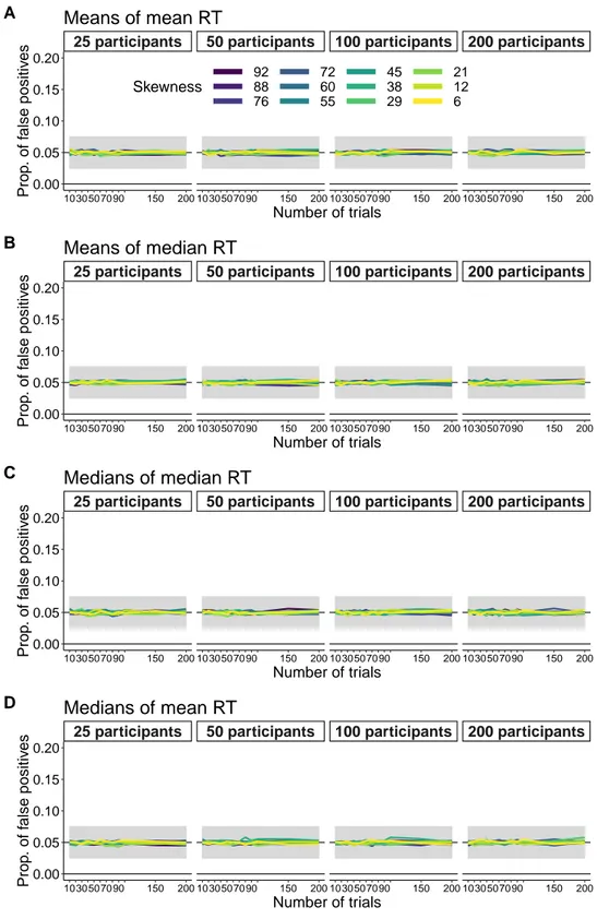
Because of this bias, Miller(1988)recommended to not use the median to study skewed distributions when sample sizes are relatively small and differ across con-ditions or groups of participants. We suspect such situ-ations are fairly common given that small sample sizes are still the norm in many fields of psychology and neu-roscience: for instance, in some areas of language re-search participants can only be exposed to stimuli once and unique stimuli are difficult to create; in clinical psy-chology, some experiments must be kept short to deal with special populations; in occupational psychology, social psychology or cognitive psychology of ageing and development, a whole battery of tests might be admin-istered in one session. However, as we demonstrate here, the problem is more complicated and the choice between the mean and the median depends on the goal of the researcher. In this article, which is organised in 5 sections, we explore the advantages and disadvantages of the sample mean and the sample median. First, we replicate Miller’s simulations of estimations from sin-gle distributions. Second, we introduce bias correction and apply it to Miller’s simulations. Third, we exam-ine sampling distributions in detail to reveal unexpected features of the sample mean and the sample median. Fourth, we extend Miller’s simulations to consider false and true positives for the comparisons of two condi-tions. Finally, we consider a large dataset of RT from a lexical decision task, which we use to contrast different approaches.
Replication of Miller 1988
To illustrate the sample median’s bias, Miller(1988) employed 12 ex-Gaussian distributions that differed in skewness (Table 1). The distributions are illustrated in Figure2, and colour-coded using the difference be-tween the mean and the median as a non-parametric measure of skewness. Figure 1 used the most skewed distribution of the 12, with parameters (µ= 300, σ = 20, τ = 300).
To estimate bias, following Miller (1988) we per-formed a simulation in which we sampled with replace-ment 10,000 times from each of the 12 distributions. We took random samples of sizes 4, 6, 8, 10, 15, 20, 25, 35, 50 and 100, as did Miller. For each random sample, we computed the mean and the median. For each sample size and ex-Gaussian parameter, the bias was then defined as the difference between the mean of the 10,000 sample estimates and the population value.
Table 1
Miller’s 12 ex-Gaussian distributions. Each distribu-tion is defined by the combinadistribu-tion of the three parameters µ (mu), σ (sigma) and τ (tau). The mean is defined as the sum of parameters µ and τ. The median was calcu-lated based on samples of 1,000,000 observations (Miller 1988 used 10,000 observations), because it is not known analytically. Skewness is defined as the difference between the mean and the median.
µ σ τ mean median skewness
300 20 300 600 509 92 300 50 300 600 512 88 350 20 250 600 524 76 350 50 250 600 528 72 400 20 200 600 540 60 400 50 200 600 544 55 450 20 150 600 555 45 450 50 150 600 562 38 500 20 100 600 572 29 500 50 100 600 579 21 550 20 50 600 588 12 550 50 50 600 594 6
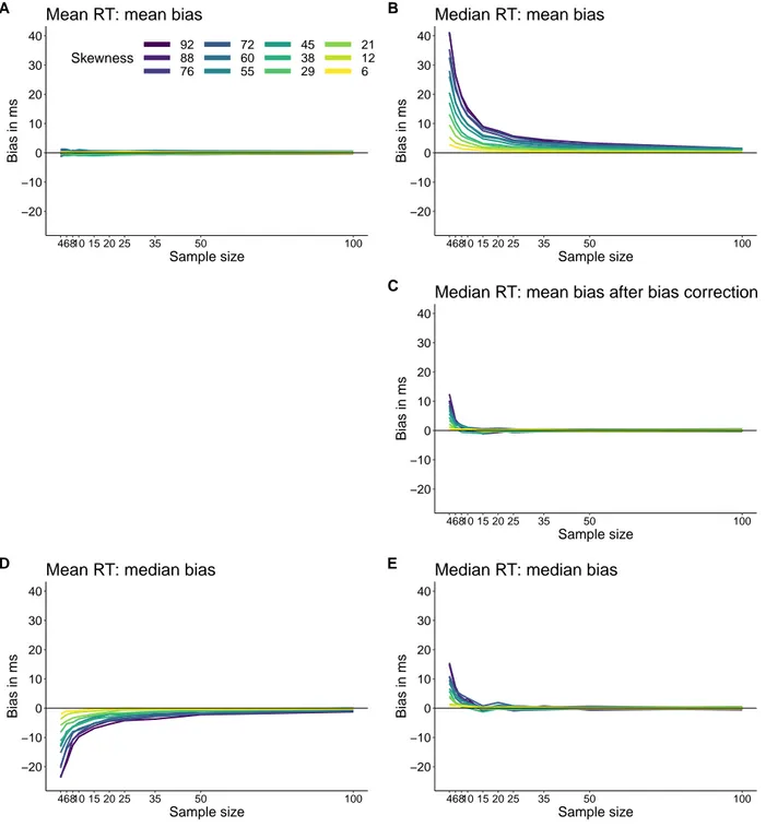
First, as shown in Figure 3A, we can check that the mean is not mean biased. Each line shows the results for one type of ex-Gaussian distribution: the mean of 10,000 simulations for different sample sizes minus the population mean (600). Irrespective of skewness and sample size, bias is very near zero — it would converge to exactly zero as the number of simulations tends to infinity.
Contrary to the mean, the median estimates are bi-ased for small sample sizes. The values from our simulations are very close to the values reported in Miller(1988)(Table2). The results are also illustrated in Figure3B. As reported by Miller(1988), bias can be quite large and it gets worse with decreasing sample sizes and increasing skewness. Based on these results, Miller(1988)made this recommendation:
’An important practical consequence of the bias in median reaction time is that sam-ple medians must not be used to compare re-action times across experimental conditions when there are unequal numbers of trials in the conditions.’
According to Google Scholar, Miller(1988)has been cited 187 times as of the 18th of April 2019. A look at some of the oldest and most recent citations reveals that his advice has been followed. A popular review arti-cle on reaction times, cited 438 times, reiterates Miller’s recommendations (Whelan,2008). However, there are
0.0000
0.0025
0.0050
0.0075
0.0100
0
250
500
750
1000
1250
1500
Reaction times (ms)
Density
Skewness
92
88
76
72
60
55
45
38
29
21
12
6
Figure 2.Miller’s 12 ex-Gaussian distributions. This figure was created using the code in the miller1988 notebook.
several problems with Miller’s advice, which we explore in the next sections, starting with one omission from Miller’s assessment: the bias of the sample median can be corrected using a percentile bootstrap bias correc-tion.
Bias correction
A simple technique to estimate and correct sampling bias is the percentile bootstrap (Efron,1979; Efron and Tibshirani, 1994). If we have a sample of n observa-tions, here is how it works:
• sample with replacement n observations from the original sample
• compute the estimate (say the mean or the me-dian)
• perform steps 1 and 2 nboot times
• compute the mean of the nboot bootstrap esti-mates
The difference between the estimate computed using the original sample and the mean of the nboot bootstrap estimates is a bootstrap estimate of bias.
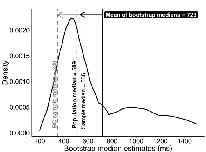
To illustrate, let’s consider one random sample of 10 observations from the skewed distribution in Figure1A, which has a population median of 508.7 ms (rounded to 509 in the figure):
sample= [355.0, 350.0, 466.7, 1758.2, 604.5, 1707.6, 367.2, 1741.3, 331.4, 1193.2] The median of the sample is 535.6 ms, which over-estimates the population value of 508.7 ms. Next, we sample with replacement 1,000 times from our sample, and compute 1,000 bootstrap estimates of the median. The distribution obtained is a bootstrap estimate of the sampling distribution of the median, as illustrated in Figure4. The idea is this: if the bootstrap distribution approximates, on average, the shape of the sampling distribution of the median, then we can use the boot-strap distribution to estimate the bias and correct our sample estimate. However, as we’re going to see, this works on average, in the long-run. There is no guaran-tee for a single experiment.
The mean of the bootstrap estimates is 722.6 ms. Therefore, our estimate of bias is the difference between the mean of the bootstrap estimates and
Table 2
Bias estimation for Miller’s 12 ex-Gaussian distributions. Columns correspond to different sample sizes. Rows correspond to different distributions, sorted by skewness. Values are for the mean bias, as illustrated in Figure3B. There are several ways to define skewness using parametric and non-parametric methods. Following Miller 1988, and because the emphasis is on the contrast between the mean and the median in this article, we defined skewness as the difference between the mean and the median.
Skewness n=4 n=6 n=8 n=10 n=15 n=20 n=25 n=35 n=50 n=100 92 41 26 19 18 8 8 6 4 3 1 88 39 27 21 16 10 7 5 5 3 2 76 35 23 16 12 8 7 5 4 3 1 72 35 24 16 14 8 6 5 4 3 2 60 28 18 15 9 6 6 4 3 2 1 55 26 18 12 9 7 5 4 3 2 1 45 21 14 10 9 5 4 3 2 2 1 38 18 11 8 7 5 3 3 1 1 1 29 13 10 6 5 3 2 2 1 1 0 21 9 6 4 4 2 2 1 1 1 0 12 5 4 3 2 1 1 1 1 0 0 6 2 2 1 0 1 0 0 0 0 0
the sample median, which is 187 ms, as shown by the black horizontal arrow in Figure 4. To correct for bias, we subtract the bootstrap bias estimate from the sample estimate (grey horizontal arrow in Figure4): sample median - (mean of bootstrap estimates - sample median)
which is the same as:
2 x sample median - mean of bootstrap estimates. Here the bias corrected sample median is 348.6 ms. So the sample bias has been reduced dramatically, clearly too much from the original 535.6 ms. But bias is a long-run property of an estimator, so let’s look at a few more examples. We take 100 samples of n = 10, and compute a bias correction for each of them. The results of these 100 simulated experiments are shown in Figure 5A. The arrows go from the sample median to the bias corrected sample median. The black vertical line shows the population median we’re trying to esti-mate.
With n= 10, the sample estimates have large spread around the population value and more so on the right than the left of the distribution. The bias correction also varies a lot in magnitude and direction, some-times improving the estimates, somesome-times making mat-ters worse. Across experiments, it seems that the bias correction was too strong: the population median was 508.7 ms, the average sample median was 515.1 ms, but the average bias corrected sample median was only 498.8 ms (Figure5B).
What happens if instead of 100 experiments, we per-form 1000 experiments, each with n= 10, and compute a bias correction for each one? Now the average of the bias corrected median estimates is much closer to the true median: the population median was 508.7 ms, the average sample median was 522.1 ms, and the average bias corrected sample median was 508.6 ms. So the bias correction works very well in the long-run for the me-dian. But that’s not always the case: it depends on the estimator and on the amount of skewness (for instance, as we will see in the next section, bias correction fails for quantiles estimated using the Harrell-Davis estimator).
If we apply the bias correction technique to our me-dian estimates of samples from Miller’s 12 distributions, we get the results in Figure 3C. For each iteration in the simulation, bias correction was performed using 200 bootstrap samples. The bias correction works very well on average, except for the smallest sample sizes. The failure of the bias correction for very small n is not surprising, because the shape of the sampling distribu-tion cannot be properly estimated by the bootstrap from so few observations. More generally, we should keep in mind that the performance of bootstrap techniques depends on sample sizes and the number of resam-ples, among other factors (Efron and Tibshirani, 1994; Wilcox, 2017). From n = 10, the bias values are very close to those observed for the mean. So it seems that in the long-run, we can eliminate the bias of the sample median by using a simple bootstrap procedure. As we will see in another section, the bootstrap bias correc-tion is also effective when comparing two groups. Be-fore that, we need to look more closely at the sampling distributions of the mean and the median.
−20 −10 0 10 20 30 40 46810 15 20 25 35 50 100 Sample size Bias in ms Skewness 92 88 76 72 60 55 45 38 29 21 12 6
Mean RT: mean bias A −20 −10 0 10 20 30 40 46810 15 20 25 35 50 100 Sample size Bias in ms
Median RT: mean bias B −20 −10 0 10 20 30 40 46810 15 20 25 35 50 100 Sample size Bias in ms
Median RT: mean bias after bias correction C −20 −10 0 10 20 30 40 46810 15 20 25 35 50 100 Sample size Bias in ms
Mean RT: median bias D −20 −10 0 10 20 30 40 46810 15 20 25 35 50 100 Sample size Bias in ms
Median RT: median bias E
Figure 3.Bias estimation. For each sample size and ex-Gaussian parameter, mean bias was defined as the difference
between the mean of 10,000 sample estimates and the population value; median bias was defined using the median of 10,000 sample estimates. A. Mean bias for mean reaction times. B. Mean bias for median reaction times. C.
Mean bias for median reaction times after bootstrap bias correction. D. Median bias for mean reaction times. E.
Median bias for median reaction times. This figure was created using the code in the miller1988 notebook.
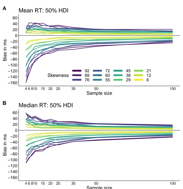
Sampling distributions
The bias results presented so far rely on the standard definition of bias as the distance between the mean of the sampling distribution (here estimated using
Monte-Carlo simulations) and the population value. However, using the mean to quantify bias assumes that this es-timator of central tendency is the most appropriate to characterise sampling distributions; it also assumes that