Evaluation of clusterings of gene expression data

Evaluation of clusterings

of gene expression data

Zelmina Lubovac

Department of Computer Science

University College of Skövde

S-54128 Skövde, SWEDEN

expression data

Zelmina Lubovac

Submitted by Zelmina Lubovac to the University of Skövde

as a dissertation towards the degree of M.Sc. by examination

and dissertation in the Department of Computer Science.

October 2000

I hereby certify that all material in this dissertation which is

not my own work has been identified and that no material is

included for which a degree has already been conferred upon

me.

___________________________________

Recent literature has investigated the use of different clustering techniques for

analysis of gene expression data. For example, self-organizing maps (SOMs) have

been used to identify gene clusters of clear biological relevance in human

hematopoietic differentiation and the yeast cell cycle (Tamayo et al., 1999).

Hierarchical clustering has also been proposed for identifying clusters of genes that

share common roles in cellular processes (Eisen et al., 1998; Michaels et al., 1998;

Wen et al., 1998). Systematic evaluation of clustering results is as important as

generating the clusters. However, this is a difficult task, which is often overlooked in

gene expression studies. Several gene expression studies claim success of the

clustering algorithm without showing a validation of complete clusterings, for

example Ben-Dor and Yakhini (1999) and Törönen et al. (1999).

In this dissertation we propose an evaluation approach based on a relative entropy

measure that uses additional knowledge about genes (gene annotations) besides the

gene expression data. More specifically, we use gene annotations in the form of an

enzyme classification hierarchy, to evaluate clusterings. This classification is based

on the main chemical reactions that are catalysed by enzymes. Furthermore, we

evaluate clusterings with pure statistical measures of cluster validity (compactness

and isolation).

The experiments include applying two types of clustering methods (SOMs and

hierarchical clustering) on a data set for which good annotation is available, so that

the results can be partly validated from the viewpoint of biological relevance.

The evaluation of the clusters indicates that clusters obtained from hierarchical

entropy often contain enzymes that are involved in the same enzymatic activity. On

the other hand, the compactness and isolation measures do not seem to be reliable for

evaluation of clustering results.

Keywords: Gene expression analysis, Evaluation of clusterings, Relative entropy,

1 Introduction ... 1

2 Background... 5

2.1 Gene expression ... 5

2.2 Analysis of gene expression ... 8

2.3 Cluster analysis ... 11

2.3.1 General definition and procedure ... 12

2.3.2 Purpose with cluster analysis in gene expression studies ... 14

2.4 Clustering algorithms ... 15 2.4.1 Similarity measures... 15 2.4.2 Self-Organizing Maps ... 17 2.4.3 Hierarchical clustering ... 21 2.5 Other techniques... 24 2.5.1 Bayesian networks ... 25 2.5.2 Supervised methods ... 25

3 Problem statement...29

3.1 Aim and objectives... 30

3.2 Hypotheses... 32

3.3 Delimitation ... 33

4 Method ...34

4.1 Data and software... 34

4.1.1 Experimental data ... 34

4.1.2 Software for analysis... 35

4.2 Suggested approaches for validation and evaluation ... 37

4.2.1 Statistical approaches ... 39

4.2.2 Metabolic simulation approach ... 44

4.2.3 Cluster-annotation correspondence... 45

4.3 Approach for evaluation in this work... 46

4.3.1 Enzyme classification ... 47

4.3.2 Entropy measure ... 49

4.3.3 Compactness and isolation ... 51

4.4 Experiments ... 55

4.5 Biological evaluation... 59

5 Results and analysis...61

5.1 Experiment 1... 61

5.1.1 Validation against enzyme classes... 64

5.1.2 Validation against functional classes ... 68

5.2 Experiment 2 ... 71

6 Conclusions ...75

7 Discussion...77

Acknowledgements ...79

References ...80

Appendix A ...86

Appendix B ...87

1 Introduction

This project deals with the area of gene expression analysis, which is concerned with

how the expression levels of thousands of genes measured by use of microarrays can

be analysed by computational methods. The purpose with such analysis is to

discover biologically meaningful patterns in the data. Data that will be used in

various experiments during this project is collected from mouse cells in different

tissues. All expression data is obtained from AstraZeneca R&D Möndal, Sweden.

The goals of the project include analysis and evaluation of the clusterings obtained

from two computational techniques for clustering multidimensional data,

self-organizing maps (SOMs) and average linkage hierarchical clustering (see section

2.4). Both clustering techniques have been used in gene expression analysis in

previous work (Törönen et al., 1999; Tamayo et al., 1999; Eisen et al., 1998;

Michaels et al., 1998; Wen et al., 1998). The importance of algorithms for clustering

the data increased considerably because of the DNA technology revolution. DNA

microarrays produce large volumes of expression data that needs efficient methods

for organising, visualising and interpreting.

The oligonucleotide arrays (also called DNA microarrays, DNA chips or Biochips)

that have been developed in the last years have made it possible to monitor the

expression levels of thousands of genes in a single experiment. At the beginning of

1999, microarrays containing 5,000 – 10,000 genes were already in use (Lander,

1999), and arrays being manufactured contained, for example, 14,000 human genes

(Brown and Botstein, 1999) or all the 3,000 Drosophilia melanogaster genes. Very

briefly explained (and in a highly simplified manner), such an array consists of a

sequences, have been attached (Southern et al., 1999). This array can be “washed”

with fluorescently tagged cDNA samples from test cells, so that sequences

complementary to the probes will hybridize. After hybridization, the amount of

fluorescence can be measured, so that the abundance of cDNA of each gene can be

measured (Brown and Botstein, 1999). Furthermore, in order to avoid the

complications of hybridization kinetics, the array spot for each gene contains a set of

probe pairs – one probe being the target sequence and the other being one of its

one-point mutants. Samples from test and reference cells are tagged with different dyes,

so that measuring the fluorescence intensity for each probe is done by measuring the

ratio of fluorescence between such a set of probe pairs (Brown and Botstein, 1999).

Microarray technology opens up tremendous opportunities for understanding cell

function by studying how the expression levels of genes are affected by

environmental factors, and also by studying which genes respond similarly to a

particular stimulus. When expression levels in experiments are measured in a series

of time steps, it becomes possible to find similar patterns of change in the expression

levels among genes participating in the same regulatory network. Hence, similar

expression profiles should be clustered in order to find genes that are co-regulated,

involved in the same mechanism, or have similar function. A number of researchers

have therefore proposed methods for clustering gene expression time-series data,

such as self-organizing maps (SOMs) (Tamayo et al., 1999), hierarchical clustering

(Michaels et al., 1998), super-paramagnetic clustering (Getz et al., 2000) and

K-means clustering (Hartigan, 1975).

However, several gene expression studies (Ben-Dor and Yakhini, 1999; Törönen et

validation of the resulting clusterings. Evaluation of the results is often restricted to

visual inspection of clusters and identifying genes, which, for instance, exhibit the

same dramatic changes between time points. There is lack of systematic approaches

to evaluate clustering results. Therefore, one of the aims of this work is to investigate

some possible approaches for cluster evaluation. Since cluster analysis of gene

expression is still in its infancy, a lot of improvements remain to be done in this

field.

Evaluation of clusterings is often considered to be the central and most complex part

in cluster analysis. Unfortunately, it often ignored in gene expression studies because

of its difficulty. In our attempt to make a contribution to the procedure for cluster

evaluation, we use a measure based on information about genes (gene annotations,

see Appendix A). In some approaches that has been suggested in previous work,

functional gene classification, which is an example of gene annotation, has been used

to analyse gene expression data (D’heaseleer et al, 1999; Zhu and Zhang, 1999). In

those studies, the correlation between expression clusters and general functional

classes has been examined, assuming that genes sharing common functions should

be regulated together. Another way to evaluate cluster quality is to compare clusters

with another indicator of similarity, for example the number of genes that share

control elements in each cluster. Fuhrman et al.1describe this procedure shortly.

In this dissertation, enzyme classification, which is another type of gene annotation,

will be used for evaluation of clusterings. The question is whether it is sufficient to

evaluate clusters by using enzyme information. Relative entropy (with respect to

1

Tracing genetic information flow from gene expression to pathways and molecular networks

enzyme number) has been used to select clusters for further investigation. This

measure has been compared to statistical indices of cluster validity, isolation and

compactness.

This dissertation is structured as follows:

Chapter 2 describes the necessary foundations of the problem area for this work.

This chapter includes sections about genes, proteins and gene expression in general

(2.1). It also gives an introduction to DNA microarrays and analysis of gene

expression data (2.2). Section 2.3 provides a description of the most common

approach to analysis of gene expression patterns, i.e. clustering algorithms, whereas

section 2.4 describes other approaches for analysis that have been applied on gene

expression data. The problem statement is described in chapter 3, while chapter 4

explains methods that have been applied in this work. Results and analysis of the

obtained results can be found in chapter 5, while chapter 6 suggests conclusions that

can be drawn from the results of this work. Finally, chapter 7 is a discussion chapter,

2 Background

This chapter provides a description of the problem area. The first section introduces

the concept of gene expression in general, while section 2.2 explains microarray

technology that allows monitoring the expression of multiple genes simultaneously,

rather than in isolation. Section 2.3 gives an introduction to cluster analysis, while

section 2.4 contains comprehensive descriptions of SOM and hierarchical clustering.

Finally, other techniques that have been applied in gene expression data analysis are

described in section 2.5.

2.1 Gene expression

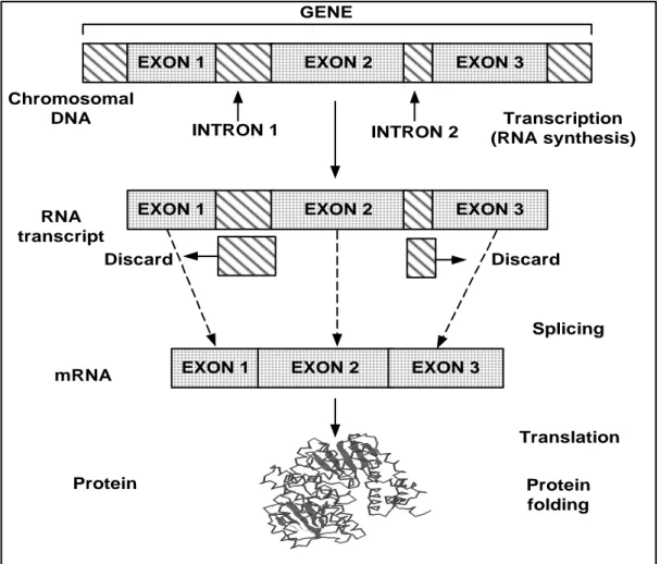
This section starts with a brief review of the expression of genetic information, i.e.

the DNA→RNA→PROTEIN flow. This flow of genetic information is known as the central dogma of molecular biology (Strachan and Read, 1996). Figure 1 shows a

schematic representation of how hereditary information that is encoded in DNA

sequences is transmitted to the protein synthesis machinery in the cell, via the RNA

EXON 1 EXON 2 EXON 3 GENE

INTRON 1 INTRON 2

EXON 1 EXON 2 EXON 3

RNA transcript

EXON 1 EXON 2 EXON 3

Protein mRNA Transcription (RNA synthesis) Chromosomal DNA Translation Protein folding Discard Discard Splicing

Figure 1: Schematic representation of genetic information processing in the cell.

In a simplified manner, we can distinguish two stages in protein synthesis –

transcription and translation. During the transcription stage, RNA polymerase uses

single-stranded DNA as a template in order to make complementary copies of DNA

information. Through the not fully understood ‘editing’ process, often referred to as

gene splicing (Brown, 1998), sequences that are not coding for proteins, called

introns, are eliminated during the formation of messenger RNA (mRNA). Processed

mRNA contains only exons, i.e. segments of DNA that are translated into proteins

(Carter and Boyle, 1998). The translation process converts information in mRNA

information for protein synthesis in the form of triplet codons. Transfer RNA

(tRNA) molecules, which enable the translation process, are provided with

anticodons corresponding to codons on mRNA. Hence, tRNA controls the matching

of codons in mRNA with amino acids. Each triplet of ribonucleotides corresponds to

a single amino acid of the polypeptide or protein (Brown, 1998). Simply stated, the

described process of gene expression is a process that allows biological information

embedded in the gene to be available to the cell in the form of protein.

It is important to highlight that only small fragments of DNA are expressed to give a

protein (Strachan and Read, 1998). Different cells, depending on the cells’

metabolism (Strachan and Read, 1998), transcribe different segments of DNA

(transcript units). Consequently, the study of gene expression levels involves

determining the amount of mRNA of those genes that are active in the cell. The level

of mRNA that is produced in the cell does not necessarily guarantee that the same

amount of the corresponding protein is produced. Despite this lack of exact

correspondence, most studies use the level of mRNA as an indicator of the amount

of protein. This can be done because of the important role mRNA plays in regulating

the protein level.

The study of gene expression has become crucial in many contexts with emphasis on

exploring and assigning functions to genes. Today, the functional information of

genes is usually incomplete for most organisms (Bassett et al., 1999). The assertion

that expression patterns of a gene provide indirect information about gene function

(Debouck and Goodfellow, 1999) is one of the reasons for the great popularity of

analysis of gene expression. The analysis of the patterns of thousands of genes

simultaneously can help us to track the gene function, which in turn facilitates e.g.

Goodfellow, 1999). Gene expression studies also benefit drug development, since

DNA chips enable monitoring the effects of drugs on gene expression (Debouck and

Goodfellow, 1999).

2.2 Analysis of gene expression

Only a decade ago, the possibility to simultaneously measure the amount of every

transcript (mRNA) in the cell seemed impossible (Bassett et al., 1999). New DNA

chip technology, also known as DNA microarrays has resulted in new possibilities of

studying gene expression. By using DNA microarrays, which consist of either

oligonucleotides or cDNA attached to a solid support, we are today able to study the

level of thousands of mRNA in parallel (Brown and Botstein, 1999). Figure 2

illustrates the steps in gene expression analysis using DNA microarrays.

1 2 3 4 5 laser excitation

Figure 2: Gene expression analysis using a DNA microarray. See text for explanation of the steps.

DNA chip technology is relatively new and it is based on base pair hybridization

for creating DNA chips, manufactured by different companies, e.g. Affymetrix,

Synteni, Nanogen etc.

Here, the method for designing DNA microarrays that has been described in Brown

and Botstein (1999) is described, because of its simplicity. This process is illustrated

in figure 2. In the first step cell samples that will be compared are chosen and the

total mRNA is isolated from different cell populations, for example mRNA samples

from vegetative and sporulating yeast cells. Captured mRNA is difficult to work

with because of its tendency of being destroyed. Hence, mRNA must be

reverse-transcribed into complementary DNA (cDNA), which is more suitable form to work

with. Total cDNA from both reference and test sample are fruorescently labelled

using different fluorescent dyes (e.g. red and green). The labelled cDNA (stage 2 in

figure 2) are called probes because they are used to probe a collection of spots on the

microarray, i.e. an array of thousands of DNA sequences printed onto a glass slide

(Duggan et al., 1999). The two sets of probes are then pooled, i.e. mixed together

(Duggan et al., 1999), and hybridized on the DNA microarray (stage 3).

Hybridization is a potential of amino acids to form base pairs with another. Probes

containing sequences that are complementary to DNA on a given spot will hybridize

to that spot. The relative abundance (in one cell sample compared to another) of

mRNA from each gene is reflected by the ratio of fluorescence measured at the array

position corresponding to that gene. Laser excitation of the targets enables detection

of the light emitted by fluorescent molecules (stage 4). Each array is scanned to

generate images recording its intensity (Cheung et al., 1999). The final step shows

the resulting image of a scanned array.

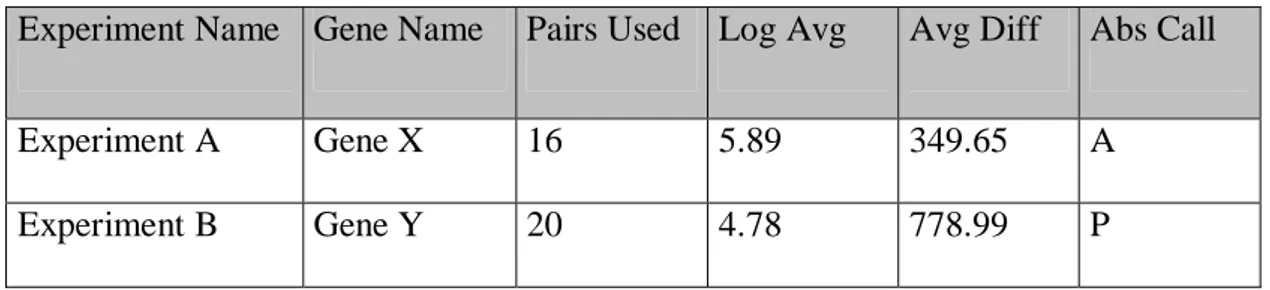
The expression analysis probe array from Affymetrix is called GeneChip. Each gene

pair consists of perfect match (PM) and mismatch (MM). Mismatch probes serve as

control probes that differ from the corresponding PM only by a single base in the

central position2). This strategy of probe redundancy allows discrimination between

the “real” signal and that occurring because of non-specific hybridization (Lipshutz

et al., 1999). Hybridization signal intensities are calculated by subtracting MM from

PM and averaging them over the probe pairs in each set. The result from this

calculation is called Avg Diff (Average difference). Avg diff is an example of data

that can be captured with the help of GeneChip technology. The figure below shows

Avg Diff together with the other types of expression data that can be analysed further

with a variety of software tools that have been developed for use in the processing of

expression data. Explanation of other terms in table 1 that need to be explained

follows below.

Experiment Name Gene Name Pairs Used Log Avg Avg Diff Abs Call

Experiment A Gene X 16 5.89 349.65 A

Experiment B Gene Y 20 4.78 778.99 P

Table 1: Example of data captured in expression analysis software.

As explained on the Research Genetics website3, Log Average Ratio (Log Avg) is

determined by computing probe pair intensity ratio (PM/MM), taking the log of

obtained values and averaging them over the probe pairs for each set.

2

For more information see www.affymetrix.com

3

Abs Call (Absolute Call) is used to determine the status of the transcript, i.e. whether

a particular probe set is present “P”, absent “A”, or marginally present “M”.

As was already stated, attributes that are shown in table 1 represent a common type

of output from array experiments. A great challenge is, however, to analyse this

output in order to convert data into information and that information into knowledge.

For that purpose, different data mining techniques have turned out to be useful.

According to Berry and Linoff (1997), data mining can be defined as

“the exploration and analysis by automatic or semi-automatic means, of

large quantities of data in order to discover meaningful patterns and

rules”

The next section explains some approaches to data mining that have been widely

used for discovering patterns in gene expression data. For further reading, there is a

review (Bassett et al., 1999) that summarises different computational applications

involved in the area of gene expression analysis, i.e. everything from image analysis

to data integration, data mining and visualisation. Here, the focus is on the method

that is of interest in this work, i.e. cluster analysis.

2.3 Cluster analysis

Since there is a tight connection between a gene’s function and its expression pattern

(Brown and Botstein, 1999), an assumption that is frequently made in many studies

is that genes should be organised according to the similarities of their expression

profiles (Bassett et al., 1999). Since the idea behind clustering methods is to group

similar data points together (Tamayo et al., 1999), this approach has been widely

applied to gene expression analysis in terms of grouping together genes with similar

description of different clustering algorithms, a general introduction of cluster

analysis with necessary terminology will be provided.

2.3.1 General definition and procedure

Cluster analysis is a statistical methodology comprising a wide diversity of

procedures that can be used to create classifications. More specifically, a clustering

method is a:

“multivariate statistical procedure that starts with data containing

information about a sample of entities and attempts to reorganize these

entities into relatively homogeneous groups” (Aldenderfer and

Blashfield, 1989, page 7).

Since cluster analysis has evolved from many different disciplines, e.g. social science

and computer science, it can be defined in many different ways. The definition above

is taken from a statistics textbook that describes clustering very generally without

being biased to reflect some specific purpose. Before we focus on cluster analysis for

the specific context of this work, gene expression, we will introduce a general cluster

analysis procedure.

Aldenderfel and Blashfield (1989) have distinguished five basic steps that normally

characterise all cluster analysis studies:

1. Selection of data to be clustered

2. Definition of variables on which to measure the entities in the data

3. Computation of similarities among the entities

4. Application of the clustering algorithm to create clusters

5. Validation of the obtained clusters

The experimental part of this work is characterised by this procedure to a great

The initial step deals with the selection of the data that is to be used in clustering.

The question that can be asked is whether it is more suitable to use artificial or

real-life data for the intended purpose.

The second step deals with the choice of variables, which is concerned with the

problem of finding variables that best reflect the concept of similarity that is used

within the context of the work. Another question that this step deals with is whether

it is suitable to transform values by, for instance, performing a logarithmic

transformation or a normalisation of data. The choices that we have made can be

found in section 4.1.1.

The third step is concerned with calculation of similarity between profiles. Section

2.4.1 provides a description of the two similarity measures that have a widespread

use in gene expression analysis and are also used in this work.

The fourth step is to apply the chosen algorithm. For some methods, this procedure

requires determining the number of clusters. It is also important to be aware of the

shortcomings of the clustering algorithms. Knowing the shortcomings and strengths

of the algorithms is important for discovering that the obtained results are, for

instance, due more to the specific characteristics of the algorithm rather that the

inherent structure of data. The algorithms that are used in this work are described in

sections 2.4.2 and 2.4.3. Section 5.4 clarifies our way of applying the chosen

algorithms, e.g. parameter settings, filtering of data etc.

The last step, which is as important as applying the algorithm and generating the

clusters, is validation of clusters. According to Aldenderfel and Blashfield (1989), in

every clustering study one needs to use some type of validity procedure to provide

evidence of cluster validity. Since this step has a great importance in this work, it is

2.3.2 Purpose with cluster analysis in gene expression studies

Different techniques for measuring gene expression result in large amounts of data

that are difficult to interpret without computational methods and needs a very careful

analysis because biological signals may be hidden by experimental noise. Hence, the

development of computational techniques for interpreting large amounts of gene

expression data is a major challenge in functional genomics. According to Eisen et

al. (1998), this research area needs a holistic approach to the analysis of genome data

that reflects the order in the whole set of observations, allowing biologists to develop

an integrated understanding of the process being studied. Other researchers, like

Fuhrman et al. (2000) for instance, uses computational methods that focus on

identification of genes that are defined as significant for the intended purpose,

instead of focusing on the whole data set. Hence, the methods that traditionally have

been performed manually by biologists, like finding genes with significant change in

expression, can be done in a more formal fashion by using different computational

techniques.

In the section 2.4, different computational methods for analysing gene expression

data will be described. Before we introduce the methods, the purpose with using

these methods as an important part of expression analysis will be clarified. Hence,

some of the purposes with gene expression analysis is to:

1. Discover new therapeutic drug targets (Fuhrman et al., 2000).

2. Group genes with correlated expression profiles or find groups of genes

participating in the same biological process (Eisen et al., 1998; Wen et al.,

3. Reveal gene regulatory networks from gene expression data (Chen, 1998;

D’haeseleer et al., 1999).

4. Compare expression data from different tissues, for instance tumor and

normal tissue (Alon et al., 1999).

5. Interpret gene expression in terms of metabolic pathways (Fallenberg and

Mewes, 19994).

2.4 Clustering algorithms

We start this section with a description of the most common similarity measures,

which are an integrated part of the clustering algorithms. The clustering algorithms

that have been used are also explained here.

Distance measures are used for demonstrating similarity or dissimilarity between

clusters (Aldenderfer and Blashfield, 1989).

2.4.1 Similarity measures

Among the most common representations of distance is Euclidean distance, which is

also frequently used in clustering studies. Euclidean distance is defined as:

where dijis the distance between objects i and j, and xikis the value of the variable k

for the object i.

4

Interpreting Clusters of Gene Expression Profiles in Terms of Metabolic Pathways.In Proceedings

(

)

∑

Another type of distance measure that is widely used is the Manhattan distance, also

known as the city-block metric (Aldenderfer and Blashfield, 1989), which is defined

as:

∑

Another kind of similarity measures that have been used in gene expression

clustering studies (Eisen et al., 1998) is correlation coefficient called Pearson

coefficient. As the name indicates, this coefficient is used to determine the

correlation between objects (Aldenderfer and Blashfield, 1989). The measure is

defined as:

(

)

∑

∑

where xkiis the value of variable k for object i, xi is the mean of all values of the

variables for object i. The value of the correlation coefficient can vary between –1

and +1, where 0 implies that no relationship between objects exists (Aldenderfer and

Blashfield, 1989).

As explained by D'haeseleer et al. (2000)5, the choice of distance measure may be as

important as the choice of clustering algorithm.

Apart from the traditional hierarchical clustering techniques, there are other

clustering techniques that have been tried in this field, e.g. SOMs (Kohonen, 1997)

and K-means clustering (Hartigan, 1975; Soukas et al., 2000).

5

Genetic Network Inference: From Co-expression Clustering to Reverse Engineering,

Because of the diversity of methods, all of these methods will not be exhaustively

reviewed. Instead, the emphasis will be on those methods that have been applied in

the context of gene expression analysis.

2.4.2 Self-Organizing Maps

Self-organizing maps (SOMs) is a type of neural network method, which belongs to

the learning category called unsupervised, competitive, or self-organizing (Kohonen,

1990). Unsupervised learning is known as “learning without a teacher” because no

answers are provided during the training. In other words, unsupervised learning

relies only on input data and the dynamics of the network, i.e. no report on the

network behaviour in relation to its weight setting progress is given (Churchland and

Sejnowski, 1992). Similarly to supervised learning, unsupervised learning can be

used to establish the finite categories of samples or classes, according to similarity

relationships of the given observations.

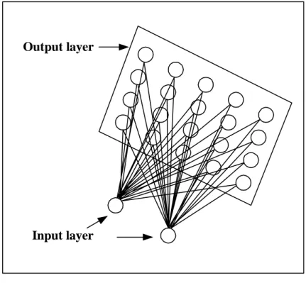
Self-organizing maps consist of a grid of processing units, called neurons. The

architecture of SOMs is often described as two-layered (see figure 3), where an input

layer consists of the vectors representing features of the problem under

consideration. The output layer, which is the two-dimensional network of nodes, is

Figure 3: Typical architecture of the SOM network, sketched from Nour and Madey (1996)

Through the learning process, the nodes on the grid become ordered so that similar

nodes are close to each other and less similar nodes far from each other (Kohonen,

1990). The minimum distance (Euclidean distance is a commonly used measure, see

section 2.3.1) defines the “winner” (Kohonen, 1990). The winner is the node in the

output map whose weight vector is most similar to the input vector. For more details

about SOMs, see the pseudocode in the figure 4 with explanations.

Input layer Output layer

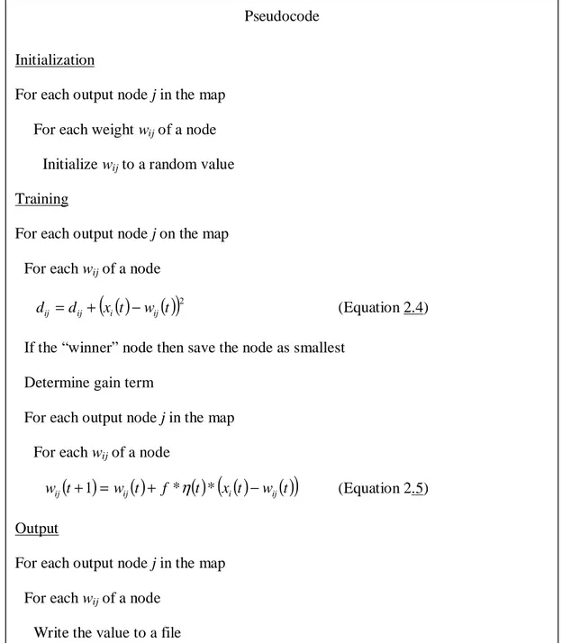
Figure 4: Pseudocode of SOM training algorithm.

As described in figure 4, in the first step of the SOM training algorithm, the weight

matrix is initialised to random values. Weight vectors of each node j in the output

layer (see figure 3) are compared to values of the input vector i. We calculate the

Euclidean distances dij(for each node j) between weight vectors and training values

by equation 2.4, where xi(t) is the input node i at time t and wij(t) is the weight from

Pseudocode

Initialization

For each output node j in the map For each weight wijof a node

Initialize wijto a random value

Training

For each output node j on the map For each wijof a node

( )

( )

(

)

If the “winner” node then save the node as smallest Determine gain term

For each output node j in the map For each wijof a node

( )

( )

( )

(

( )

( )

)

wij +1 = ij + *η * i − ij (Equation 2.5)

Output

For each output node j in the map For each wijof a node

input node i to output node j at time t. The node with the smallest Euclidean distance

represents the “winner”, i.e. the best matching unit, as explained in Kohonen (1990).

The next step in the training is to move the weights of the winning node j toward the

values of the corresponding input vector i (equation 2.5). The size of movement of

the winner’s weights is determined by the gain term

η

( )

vector and the corresponding weights, by which the winning node has its weights

updated. The neighbouring nodes also move their weights, in order to achieve a

better correspondence to the training vector (equation 2.5). At each training step, all

nodes within the neighbourhood are updated, whereas nodes outside the

neighbourhood are left intact. The radius of the neighbourhood can be time-variable.

For global ordering of the map, one should start with a fairly wide neighbourhood

and let it shrink monotonically. If the neighbourhood is too small in the beginning,

the map will not be ordered globally (Kohonen, 1990).

The neighbourhood function f in equation 2.5 controls how neighbouring nodes will

adjust their weights, i.e. f equals zero outside the neighbourhood and one for the

winner node. Within the neighbourhood, neighbourhood functionf(t)=

η

( )

represent groups of similar input vectors (clusters). The result can be used as a basis

of further analysis.

SOMs are well suited for exploratory data analysis (Tamayo et al., 1999; Nour and

Mandey, 1996), because they facilitate understanding of the underlying structure of

the data set. There are, however, some fundamental problems with this method,

problems is the determination of the number of clusters present in the data

(Mangiameliet al., 1996). In SOMs, one chooses a geometry of nodes, for example a

5x6 grid. There are no strict rules of how to choose the appropriate number of nodes.

According to Tamayoet al. (1999), it is easy to explore the structure by varying the

SOM’s geometry. By adding more nodes, tight and more distinct clusters appear,

until we reach the point at which adding new nodes does not supply the clustering

with fundamentally new patterns. The SOM geometry at that point can be

appropriate.

More details about how SOMs are used in this work, i.e. which computer package

has been used, the choice of geometry and other parameters, data pre-processing etc.,

can be found in Chapter 4.

2.4.3 Hierarchical clustering

Another type of clustering, called hierarchical clustering, is able to expose inherent

relationships that exist in the resulting clusters (Kohonen, 1997).

An important objective of hierarchical cluster analysis is to visualise the data that is

to be interpreted. A common way of representation in hierarchical clustering is a tree

structure called a dendrogram. Dendrograms illustrate division or merge

relationships between clusters, depending on whether the algorithm is divisive or

Figure 5: Dendrogram.

Divisive methods successively separate objects in one cluster into smaller clusters. In

contrast to divisive methods, agglomerative clustering starts with a number of

clusters, each containing a single object, and gradually merges those smaller clusters

into larger ones, through a series of successive steps, until we obtain a single cluster

containing all objects (Jain and Dubes, 1988).

The basic procedure of agglomerative methods can be explained by the following

steps (Everitt, 1993):

Start with n clusters C1, C2,…, Cn, where each cluster contains a single

object (individual).

1. Find the nearest pair of distinct clusters, e.g. Ci and Cj, and merge

them into one cluster Ck. Delete Ci and Cj and decrease the cluster

counter by one.

2. If the number of clusters is equal to one, then stop, otherwise return

to step 1. 6.0 5.0 4.0 3.0 1.0 2.0 0

a

b

c

d

e

Distance

Hierarchical clustering has proven valuable in studies of gene expression (Wenet al.,

1998; Spellman et al., 1998; Eisen et al., 1998; Alon et al., 1999). Some of those

studies are summarised below.

Wen et al. (1998) have in their study examined the patterns of gene expression of

112 genes that have an important role during development of the rat spinal cord.

They used the FITCH software, which is an implementation of the hierarchical

algorithm from the PHYLIP package (Felsenstein, 1989), in order to cluster gene

expression time series. Genes are clustered according to similarities in their

expression patterns determined by Euclidean distance (see section 2.4.1). This study

resulted in the five basic patterns of gene expression, called “waves”, where four

“waves” correspond to the phases in rat spinal cord development and the fifth

“wave” is largely invariant. They also mapped expression clusters to main functional

gene classes and found a correspondence between distinct functional classes and

particular expression profiles.

Eisen et al. (1998) analysed data collected from DNA microarrays, that were

designed to study gene expression in the budding yeast Saccharomyces cerevisae

during diauxic shift, the mitotic cell division cycle, temperature and reducing shocks

and sporulation. They used hierarchical clustering based on the average linkage

method. The method starts from the highest value in the similarity matrix, which is

calculated on the basis of similarity between each pair of genes by using a

modification of the Pearson correlation coefficient (see section 2.4.1). A first node in

a dendrogram (see example of a dendrogram in figure 5) is obtained by merging

those two genes that have the highest value, i.e. similarity score (Eisenet al., 1998).

The average value of observations of the merged elements is assigned to that node

only one element is left. As a complement to the dendrogram, Eisen et al. (1998)

used a colour scale to represent quantitative expression data (e.g. red colour with

varying intensity for illustration of up-regulated genes and green for down-regulated

genes). Their approach resulted in some tight clusters with genes that share similar

function, e.g. a cluster containing eight histone genes, which are known to be

co-regulated and transcribed at a particular point of the cell cycle. Hence, this study

gave some evidence that expression data in some cases has tendency to organise

genes into functional classes. However, it is unclear how those clusters containing

functionally related genes have been selected.

2.5 Other techniques

Since one of the purposes of this work is to identify open problems in the area of

gene expression analysis, it is important to not limit the work to studying only one of

the proposed analysis methods. Therefore, this work will include a survey of other

possible approaches to the analysis of gene expression patterns. The experimental

part of this work will be based on analysis with clustering algorithms, since such

analysis has proven to be useful in discovering genes that are co-regulated (Friedman

et al., 2000). Although unsupervised methods may be adequate in many cases, it is

important to highlight that those methods are not always sufficient to exploit the

richness of microarray data. Several other techniques have been proposed but they

have not attracted as much attention as unsupervised methods. Other techniques will

be introduced only as part of a literature survey, with the explicit purpose to provide

a broad foundation for a discussion on future work, identify open questions and give

a more complete picture of this research area. Below, some proposed approaches for

2.5.1 Bayesian networks

A Bayesian network is a well-known statistical tool that has been used to analyse

expression data. Friedman et al. (2000) proposed this approach for discovering

interactions between genes. The approach is built on using Bayesian networks for

representing statistical dependencies. Such a network is a graph-based model that

describes dependencies between multiple quantities that interact with each other, for

instance expression levels of different genes. This probabilistic framework is,

according to Friedmanet al. (2000), capable of learning complex relations between

genes. Bayesian networks have the potential to capture causal relationships, such as

transcriptional regulation, which are only partially reflected by clustering of

expression profiles. Bayesian networks can also integrate prior knowledge. However,

huge numbers of variables (thousands) are needed to model the complex interactions

between genes, which is difficult to handle.

2.5.2 Supervised methods

Currently, most approaches to the computational analysis of gene expression data

attempt to do classification of genes in an unsupervised fashion, i.e. in the absence of

pre-defined knowledge about genes. Recently, knowledge-based approaches, in

terms of different supervised learning methods, have also been applied on gene

expression data. Supervised learning methods use a training set to specify in advance

which data should be clustered together. Supervised methods utilise, for instance,

prior knowledge about gene function to extract information about unknown genes

from gene expression data (Brownet al., 2000).

Support vector machines (SVMs) is one of the supervised learning approaches.

When we apply SVMs on gene expression data, we start with a set of genes that

that particular functional category is collected. A training set can be assembled by

combining data from those two sets. Through the training process, SVMs learn to

distinguish members of a given functional class from non-members (Brown et al.,

2000). Learning is based on expression features of the functional class. SVMs use

that information for any gene in order to determine the gene’s probability of being a

member of the group on which it was trained (Brownet al., 2000).

Suppose that each vector X→ represents gene expression values for a certain gene as a

point in an n-dimensional expression space. Theoretically, we can separate the

members of a given functional class from non-members by constructing a

hyperplane in expression space (Brown et al., 2000). However, it is not always

possible in practice to separate positive examples (members) from negative examples

(not-members), since most real-world problems include non-separable data. By

mapping data to a space with higher dimensionality and define a separating

hyperplane there, this problem can often be avoided. This space is known as feature

space, whereas the input space includes the training examples. Support vector

machines (SVMs) can locate the separating hyperplane by defining the function,

called kernel function, which plays the role of the dot product in the feature space.

Brown et al. (2000) explain the kernel function in terms of gene expression as

K(X,Y)=X * , which is a dot product in the input space that is used to measure→ Y→ similarity between the genes X and Y. Since they use a set of 79-element gene expression vectors, which represent expression of genes that have been measured in 79 different DNA microarray experiments, the kernel in this example equals

∑

79

1 *

Brown et al. (2000) used SVMs to analyse 2,467 genes from budding Saccharomyces cerevisiae that were measured in 79 DNA microarray experiments. Their experiment focused on learning to recognise six functional classes from the Munich Information Centre for Protein Sequences Yeast Genome Database (MYGD6). The class definitions from MYGD result from biochemical and genetic studies.

Furthermore, in Brown et al. (2000), the classifying power of SVMs was compared with four other machine learning algorithms: Parzen windows, Fisher’s linear discriminant and two decision tree learners. The comparison of performance was based on the classifier’s power of identifying positive and negative examples in the test sets. According to Brown et al. (2000), SVMs performed better than all the other techniques.

Decision trees is another machine learning technique that has been tried in this field. Similarly to the approach described above, decision trees deal with classification. Decision trees are rooted, usually binary, trees with classifiers placed on each internal node and classification placed at each leaf. Each non-leaf node is connected to a test, which splits the node’s set of possible answers into subsets that agree with possible test results. The same procedure is then recursively applied on the child nodes.

As explained in Brazma (1998), decision trees have been used to find rules predicting gene functional classes for unclassified genes, based on their expression levels at various time points. This goal was part of a bigger project, which aimed to study some aspects of the yeast metabolism and gene regulation during diauxic shift.

For this purpose, 3,347 genes with known functional classes were selected. Whether it is useful to use decision trees for the mentioned purpose or not is still unclear, i.e. it is not clear from Brazma (1998). The preliminary conclusion was that either no correlation exists between functional classes and expression profiles (which is opposite to the result from Eisen et al. (1998)) or they were dealing with non-reliable annotations. However, the project was in its initial phase when described in Brazma (1998), and the answer to this question remains to be seen.

3 Problem statement

As was already stated there exists a tremendous diversity of clustering algorithms. Furthermore, if we take into consideration various distance measures and the ways of combining them with algorithms, the number of combinations increases considerably. The question is, which clustering method is likely to be most useful for the intended domain? Aldenderfer and Blashfield (1989, page 16) state that “what is obviously needed are techniques that can be used to determine what clustering method has discovered the most “natural” groups in a data”. Aldenderfer and Blashfield (1989) defined this problem at a general level, without referring to any particular discipline or research area.

The same problem is observed in the studies concerning clustering techniques in gene expression analysis. D’haeseleer et al.7point out that different clustering methods can give different results and therefore should be treated with caution. D’haeseleer et al. continue their discussion by claiming that it is not clear which clustering methods are most useful for gene expression analysis. In order to be able to compare how different clustering algorithms performed in clustering, we need a procedure that will allow systematic evaluation of the results obtained from clustering.

D’haeseleer et al. suggest one possible way of enabling evaluation and comparison of the clustering results obtained from different algorithms. The suggested method consists of using artificial data, generated from models of regulatory networks, as a measure for comparing.

7

Genetic Network Inference: From Co-expression Clustering to Reverse Engineering,

3.1 Aim and objectives

The aim of this project is:

To develop a method for evaluation of the results obtained from different clustering techniques in gene expression analysis.

In order to achieve this aim, the following objectives need to be attained:

• Identify existing evaluation and validation approaches

• Choose suitable data and annotations

• Choose a suitable measure that will allow evaluation of clusterings

• Choose clustering algorithms

• Apply chosen evaluation and validation approaches on test data

• Evaluate how well different measures performed in evaluation of clusterings

• Evaluate how well the algorithms performed in creating “correct” clusters

Systematic evaluation and validation procedures is a not very well understood part of the cluster analysis and is therefore avoided in many studies. Several statistical validation techniques, like cophenetic correlation and significance tests on the variables used in cluster analysis, have serious problems and are not considered to be useful (Aldenderfer and Blashfield, 1989). The lack of a systematic evaluation approach is a serious problem, because we know that different clustering algorithms generate different solutions when applied to the same data set. The difficulty of evaluating how “good” the clustering is in the context of gene expression analysis is due also to the fact that we usually do not know the correct answer to the problem. In other words, how can we assess which clustering algorithm performed better in revealing biologically correct information from expression data when we often do

not know which clusters are biologically correct and which clusters are only accidental artefacts of the data?

Several studies describe evaluation of the results from different clustering methods based on their ability to recover structure in data sets with known structure. Most of them used artificial data. Mangiameli et al. (1996) evaluated, for instance, performance of SOM and different hierarchical clustering methods, by using artificial data with some imperfections like presence of outliers, irrelevant variables etc. Results from this work were that SOM was superior in both accuracy and robustness. However, the pure statistical evaluation may not always be sufficient, especially when we deal with real-life data, like gene expression data for instance. We need other criteria for evaluation that will reflect the biological nature of the data. Hence, our criterion for evaluation is based on using gene annotations. An example of gene annotation for certain gene can be the protein family that each gene belongs to, chromosomal location of the gene, enzyme class of the gene etc. (see Appendix A) For the purpose of this work, annotation needs to facilitate dividing the genes into natural groups. Sections 4.3.1 and 4.3.2 account for our choice of annotation and how we use it for the intended purpose of this work.

The next objective concerns the question how we can use gene annotation in an evaluation approach, i.e. which measure based on gene annotation can allow comparison of different clusters. It is also desirable to have a measure that will enable judging the quality of the whole clustering. Our choice of measures is presented in section 4.3.

There are many clustering algorithms and it would be impossible to test all of them. We have focused on two clustering algorithms that are considered to be useful in

gene expression analysis, SOM neural network method (see section 2.4.2) and hierarchical average linkage clustering (see section 2.4.3). It would also be interesting to compare the outcome from those two methods. Tamayo et al. (1999) claim that SOM is more suitable for gene expression analysis then hierarchical because it facilitates easy visualisation and interpretation. According to Tamayo et al. (1999), hierarchical clustering is more suitable to “situations of true hierarchical descent” such as in evolution of species but it is not suitable to reflect the multiple distinct ways in which expression patterns can be similar. On the other hand, Eisen et al. (1998) provide strong evidence that hierarchical clustering can be useful in gene expression analysis.

The next objective deals with evaluation of clusterings with the chosen measures. We want to be able to rank clusters according to their “biological correctness” and perform qualitative evaluation on complete clustering with respect to statistical and annotation-based measure. We measure the degree of correlation between clustering results and two type of annotations, namely functional categorisation and enzyme categorisation.

The last objective reflects our attempt to be able to state which algorithms performed better in creating clusters with respect to our evaluation criteria.

3.2 Hypotheses

As stated before, our criteria for evaluation of clusterings is based on a measure that relies on gene annotations. We use annotations in the form of enzyme classification that divides genes in natural groups according to their enzymatic activity. The following hypotheses will guide this project:

Using an annotation based measure for evaluation of clusterings in gene expression analysis is more reliable than purely statistical evaluation.

Hypothesis 2:

Evaluation that relies on an annotation-based measure can show which algorithm performed better in clustering gene expression data.

3.3 Delimitation

There are many kinds of gene annotations, like chromosomal location, metabolic pathway that the gene participates in, enzyme classification etc. Enzymes, which compose a large fraction of genes, can be precisely characterised by the reactions that they catalyse. Hence, genes can be naturally grouped in six main classes according to enzymatic reactions. This annotation is characterised by a hierarchy with four levels. At the bottom of the hierarchy the catalysed reactions are very specific. We will only take into consideration the first level, because we will investigate if the clusters reflect the main functionality of the enzymes and which clustering method performed better with respect to that property. Specific details like for instance which acceptor is involved in the reaction are therefore not interesting for the purpose of this work.

4 Method

This chapter provides a description of approaches that have been used in this work in order to achieve the aim. It starts with a description of the sources of the experimental data that have been used and the choice of clustering algorithm that has been applied on the experimental data. Furthermore, the section provides a review of the identified approaches for evaluation of clusterings of gene expression data and the approach that is used in this work.

4.1 Data and software

This section provides a short description of the data that has been used in the experiments. It also provides an overview of the software that has been used to cluster and visualise data.

4.1.1 Experimental data

All data that has been used in this work was obtained from AstraZeneca R&D Möndal, Sweden. The data set that we mainly focused on comes from oligonucleotide microarrays that allow expression monitoring of 6,500 genes in Mesenterial fat tissue in obese diabetic mice. The main reason for choosing this data set is that the data is well annotated, i.e. we have annotations in the form of genes’ function, localisation, enzyme hierarchy, pathway hierarchy etc. for the known genes. This annotation will be used in biological evaluation of clustering results. Another reason is that we are acquainted with the experiment for which purpose this data has been collected, for instance possible candidate genes for obesity in adipose tissue.

Data that we are working with is multidimensional. Expression levels have been measured at three time points, namely day zero, day three and day seven. Gene

expression at a time point zero corresponds to the placebo group of mice, while two remaining time points represent the gene expressions concerning groups of mice that have been treated with a substance called rosiglitazone for three and seven days respectively. Rosiglitazone is one of the three existing thiazolidinediones (TZDs), which are drugs that enhance glucose uptake by the muscle and adipose tissue and hence decrease insulin resistance (Raskin et al., 2000). Hence, this drug is useful in treatment of Type II diabetes (diabetes mellitus) that is characterised by insulin resistance, which in turn can be caused by obesity (Koppelman, 2000).

4.1.2 Software for analysis

In this work, an implementation of SOM called GENECLUSTER has been used in the analysis of gene expression data. The GENECLUSTER package was developed at Whitehead/Massachusetts Institute of Technology Center for Genome Research and is freely available8.

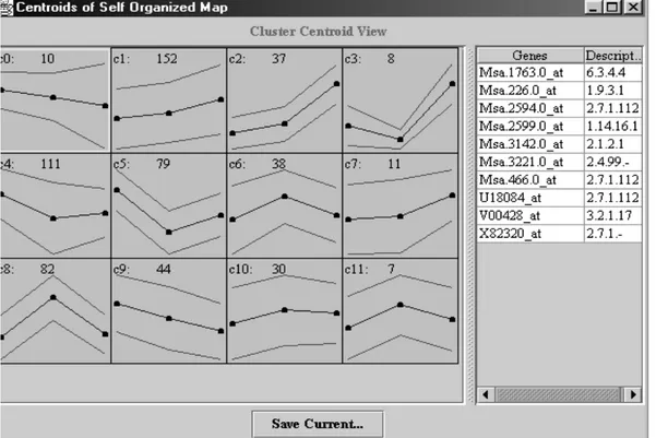
Figure 6 illustrates an example of a gene profile that has been generated and visualised by GENECLUSTER. The geometry of SOM map that has been chosen for the illustrative purpose is 3X4. For each cluster in the figure, centroids (mean) and the standard deviations, calculated from the elements in each cluster are displayed. Furthermore, we can see cluster numbers (c1, c2,…,c6) and the number of genes in each cluster (the number next to the cluster number). By clicking on each cluster, all genes that belong to that cluster and the corresponding gene descriptions are shown in the right side of the figure. When we save clustering results, two output files are created: one with the list of centroids that are in normalised form and one showing

8

the normalised data with the cluster number that each gene belongs to. Those output files are very suitable for further analysis.

Figure 6: Cluster display obtained from GENECLUSTER.

The second software package that we use for hierarchical clustering contains two programs9: Cluster and TreeView. For hierarchical clustering, Cluster provides three different options: Average linkage, single linkage, and complete linkage clustering. Cluster organises and analyses data while TreeView allows visualisation of the output obtained from Cluster. Figure 7 shows a cluster display where the primary data table is represented graphically by colouring cells in proportion to the fluorescence ratio. A more detailed description of the algorithm and the qualitative graphical analysis with help of TreeView was given in section 2.4.3. Considering similarity measures, Cluster does not provide many options. We can choose a

9

This software was developed by Michael Eisen at Stanford University and is freely available at http://rana.stanford.edu/software.

modified Pearson correlation (see section 2.4.3) that can be varied in four different ways.

When we perform clustering, Cluster produces three input files. One of the files contains input data, which is organised to reflect clustering results. Two other files show the history of merging the nodes in the gene or array clustering.

Figure 7: Cluster display obtained from Cluster and TreeView. The tree is taken from Eisen et al. (1998) by courtesy of Eisen.

4.2 Suggested approaches for validation and evaluation

In this section, some methods that have been suggested for validation and evaluation of clustering algorithms will be reviewed. Some of the methods are traditional (see

section 4.2.1), i.e. applied on clustering in general, while other methods are more specific for gene expression clustering studies (see sections 4.2.2 and 4.2.3).

We have classified these approaches in three main classes that will be described in section 4.2.1 to 4.2.3. Those classes are not disjoint, i.e. there are some methods that are overlapping. We have done this classification anyway in order to achieve a clear structure over the identified approaches.

It is also important to add an explanation regarding the usage of the concepts evaluation and validation in the text below. There is a confusion of ideas in the gene expression literature concerning those two concepts. Slonim et al. (1999) use the expression “validating the clusters” to explain the procedure of showing that discovered clusters are biologically interesting, rather than accidental artefacts of the data. According to Jain and Dubes (1988), cluster validation is the procedure of evaluating the results of cluster analysis in a quantitative and objective fashion. The latter definition considers cluster validity as determining the merits of clustering structures in a quantitative manner by examining statistically based indices (some of those indices are explained in sections 4.2.1 and 4.3.3). The same procedure is however called “evaluating clustering procedure” by Milligan (1996). Milligan (1996) also uses the term validation to refer to the same procedure. Hence, those two terms will be used interchangeably in the following sections.

During the literature survey, we have come across many different validation approaches. By taking into consideration the problem defined in chapter 3, some approaches have been excluded, partly due to the nature of the problem and partly because they were considered as inappropriate for this application area. The approaches that are reviewed below (see sections 4.2.1-4.2.3) focus on investigating

the validity of the clustering that also should allow comparison between alternative clusterings.

By way of introduction, a more general overview of statistical methods for cluster validation (Jain and Dubes, 1988) will be given, followed by the methods proposed for validating clustering for gene expression data that allow comparison between different clustering algorithms.

4.2.1 Statistical approaches

Jain and Dubes (1988) define cluster validation as a method that evaluates the results of cluster analysis in a quantitative and objective fashion. However, this definition considers clustering in general, without referring to any particular application area. D’haeseleer et al. (2000) points out that is impossible to objectively evaluate how “good” a particular clustering is without referring to what the clustering is used for. In this work we will investigate whether those statistical methods of evaluation are applicable for validation in this particular area of gene expression analysis.

Jain and Dubes (1988) describe three types of criteria and a number of indices that can be used for defining the validity of a clustering structure. Those are external, internal and relative criteria. Defined criteria should reflect a strategy by which a clustering structure is to be validated, while an index is a statistic measure that allows validity to be tested. External criteria are used in order to measure the performance of a clustering algorithm through comparing a clustering structure to a priori information. An example that Jain and Dubes (1988) refers to is using external criteria to measure the degree of correspondence between cluster categories and category labels that have been assigned in advance. Internal criteria refer to measuring how well the obtained partitions of clusters agree with the proximity

matrix, for instance. Finally, relative criteria can be used to determine which of two structures is more appropriate for the data. For instance, a relative criterion can be used to measure quantitatively whether an average link or single link structure fits the data better.

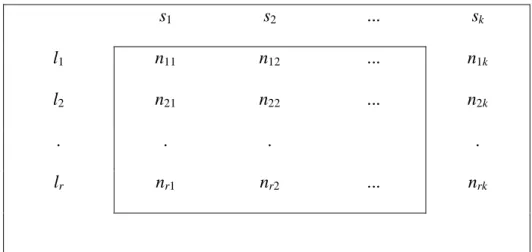
Furthermore, Jain and Dubes (1988) distinguished three types of structures, namely hierarchies, partitions and clusters. For each type of structure, they described internal, external and relative indices that can be used to test the validity of the structure. Some examples are described below in order to clarify how different indices can be used. Table 2 shows a contingency table that can be constructed from the two partitions S={s1, s2, s3,…, sk} and L={l1, l2, l3,…, lr}.

s1 s2 ... sk

l1 n11 n12 ... n1k

l2 n21 n22 ... n2k

. . . .

lr nr1 nr2 ... nrk

Table 2: Contingency table for two partitions

Jain and Dubes (1988) describe how external indices, which can be used for assessing the degree to which two partitions of n objects agree, can be expressed in terms of contingency tables. One partition s can be the result of applying clustering algorithms on expression data and the second partition l can consist of predefined

elements, independent of the first partition. The number of objects that are both in partition uiand in partition vjis denoted with entry nij.

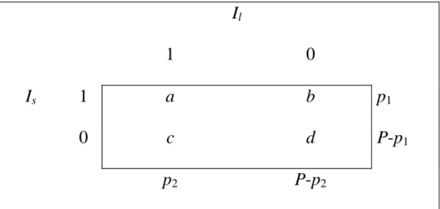
Another way of expressing external indices is to use an indicator function, which is exemplified in table 3. Suppose we have n objects {x1, x2, x3,…, xn}. An indicator

function can, for instance, be defined as:

Is(i,j)= ⎩ ⎨ ⎧ ∈ ∈ ≤ ≤ otherwise 0 1 some for and if 1 xi sk xj sk k K Il(i,j)= ⎩ ⎨ ⎧ ∈ ∈ ≤ ≤ otherwise 0 1 some for and if 1 x_i l_r x_j l_r r R

Assume that two partitions S and L are derived in the same way as is shown in the previous example. Then, Is(i,j) is 1 when objects xi and xjare in the same cluster and

0 if they are not. Similarly, Il(k,r) equals 1 when objects have the same category label and 0 if they not.

For those two indicator functions, the contingency table is shown in table 3.

Il

1 0

Is 1 a b p1

0 c d P-p1

p2 P-p2

The contingency table shows the numbers of ways in which the pairs of objects can appear in the two partitions. Jain and Dubes (1988) define a as the number of pairs of objects that can be found in the same cluster in both partitions, b as the number of pairs of objects that are in the same cluster in partition s but not in l, c as the number of pairs of objects that are in the same cluster in partition l but not in s, and d as the number of objects that are in different clusters in both partitions.

Some common indices that can be used for analysing correlation between two partitions are the HubertΓindex and the Jaccard index (Jain and Dubes, 1988). The Hubert index is defined as:

The Jaccard index is defined as:

The Hubert index will be used in biological evaluation (see section 4.5).

Another index for validating clusterings, or more precisely hierarchical structures, is the cophenetic correlation measurement that is described in Aldenderfer and Blashfield (1989). This is an internal index that can be used to determine how well the tree resulting from the hierarchical agglomerative type of clustering (dendrogram, see figure 5) corresponds to the similarities between the objects that are involved in the clustering. In order to compute the cophenetic correlation for a certain clustering, we start from the dendrogram corresponding to that hierarchical clustering solution. A similarity matrix with similarities between each pair of objects

) )( ( 1 2 2 1 2 1 p P p P p p p p Pa H − − − = Equation 4.1 c b a a J + + = Equation 4.2

is calculated from the dendrogram. Each position in the similarity matrix represents a value at which two objects have been merged into a shared cluster. Suppose that we haveN objects that have been clustered. Since hierarchical agglomerative clustering requires N-1 merger steps, the similarity matrix must have at most N-1 entries containing unique values (Aldenderfer and Blashfield, 1989). The original similarity matrix contains, on the other hand, N*(N-1)/2 unique values. According to Aldenderfer and Blashfield (1989), the cophenetic correlation for the particular clustering is the correlation between the values in the original and implied similarity matrix. The cophenetic correlation is defined as:

(

)(

)

(

) (

)

∑

∑

where Xij is distance between objects i and j in the original similarity matrix, Yij is

the distance between objects i and j from the matrix generated from a dendrogram

and x and y are the average ofXandY, respectively.

Although this is a widely used quality criterion for clustering, it is important to

highlight that there are some shortcomings with this measurement. Aldenderfer and

Blashfield (1989) point out that the two distance matrices, which serve as basis for

the calculation of cophenetic correlation, contain quite different information, since

the implied matrix has much fewer unique values then the original matrix. Another

study that has been done by Holgersson (1978) shows also that cophenetic

correlation can be a misleading indicator to clustering quality in many cases. This

validation technique does not make it possible to compare clustering solutions from

different clustering methods, since it is only applicable on hierarchical agglomerative

clustering (Aldenderfer and Blashfield, 1989).