02:10 The Impact of Spatial Variability of Hydrogeological Parameters - Monte Carlo Calculations Using SITE-94 Data

(1)

SKI Report 02:10

The Impact of Spatial Variability of

Hydrogeological Parameters - Monte

Carlo Calculations Using SITE-94 Data

António Pereira

Robert Broed

March 2002

(2)

(3)

SKI perspective

Background

In SKI’s deep repository performance assessment project SITE-94 real field data were used on a hypothetical repository for spent nuclear fuel. The project dealt with among other things radionuclide transport calculations in fractured crystalline rock. These calculations were not as comprehensive as was intended from the beginning, especially in the area of probabilistic treatment of hydrogeological parameter uncertainties.

Purpose of the project

The purpose of this project is to elucidate the influence the uncertainties in the

hydrogeological parameters have on the radionuclide release to the biosphere. Results from the hydrogeological modelling in SITE-94 are used directly in the

one-dimensional radionuclide transport model.

The uncertainties of hydrogeological parameters, Darcy velocity and longitudinal dispersion, together with transport parameters are investigated in Monte Carlo simulations. The Monte Carlo simulations are performed for five radionuclides.

Results

Monte Carlo simulations in which both the hydrogeological and transport parameters are varied simultaneously show considerable spread in the distribution of the peak release rate, compared to when only the hydrogeological parameters are varied. Hence the spread of peak releases is more influenced by the uncertainty of the transport parameters and less by the spatial variability of the hydrogeological parameters. One should, however, bear in mind that there is a synergetic effect between flow and transport phenomena, the impact of which is difficult to disentangle. The number of radionuclides in the investigation is also limited.

From the Monte Carlo simulations one can also conclude that correlations between the two hydrogeological parameters have no appreciable impact on the mean peak value of the maximum releases from the repository.

Effect on SKI’s work

This project has clearly shown a useful way to incorporate results from hydrogeological modelling directly into radionuclide transport calculations. This is important knowledge in developing SKI’s own capability to perform radionuclide transport calculations.

Project information

Responsible at SKI has been Benny Sundström. SKI ref.: 14.9-990240/99043.

Relevant SKI report: SKI Report 96:36, SKI SITE-94 Deep Repository Performance Assessment Project, December 1996.

(4)

(5)

SKI Report 02:10

The Impact of Spatial Variability of

Hydrogeological Parameters - Monte

Carlo Calculations Using SITE-94 Data

António Pereira

Robert Broed

Department of Physics

Center of Physics, Astronomy and Biotechnology

AlbaNova University Center

Stockholm University

SE-106 91 Sweden

March 2002

This report concerns a study which has been conducted for the Swedish Nuclear Power Inspectorate (SKI). The conclusions and viewpoints presented in the report are

Research

(6)

(7)

Abstract

In this report, several issues related to the probabilistic methodology for performance assessments of repositories for high-level nuclear waste and spent fuel are addressed. Random Monte Carlo sampling is used to make uncertainty analyses for the migration of four nuclides and a decay chain in the geosphere. The nuclides studied are caesium, chlorine, iodine and carbon, and radium from a decay chain.

A procedure is developed to take advantage of the information contained in the

hydrogeological data obtained from a three-dimensional discrete fracture model as the input data for one-dimensional transport models for use in Monte Carlo calculations. This procedure retains the original correlations between parameters representing different physical entities, namely, between the groundwater flow rate and the hydrodynamic dispersion in fractured rock, in contrast with the approach commonly used that assumes that all parameters supplied for the Monte Carlo calculations are independent of each other.

A small program is developed to allow the above-mentioned procedure to be used if the available three-dimensional data are scarce for Monte Carlo calculations. The program allows random sampling of data from the 3-D data distribution in the hydrogeological calculations.

The impact of correlations between the groundwater flow and the hydrodynamic dispersion on the uncertainty associated with the output distribution of the

radionuclides’ peak releases is studied. It is shown that for the SITE-94 data, this impact can be disregarded.

A global sensitivity analysis is also performed on the peak releases of the radionuclides studied. The results of these sensitivity analyses, using several known statistical

methods, show discrepancies that are attributed to the limitations of these methods. The reason for the difficulties is to be found in the complexity of the models needed for the predictions of radionuclide migration, models that deliver results covering variation of several orders of magnitude. Correlations between parameters also make it difficult to separate the contribution from each parameter on the output. Finally, it is concluded that even in cases where correlations between parameters can be disregarded for the sake of the uncertainty analysis, they cannot be disregarded in the sensitivity analysis of the results.

A new approach for global sensitivity analysis based on neural networks has been developed and tested on results for the peak releases of caesium. Promising results have been obtained by this method, which is robust and can tackle results from non-linear models even when there are correlations between parameters. This represents a considerable improvement over the capabilities of the commonly used traditional statistical methods.

(10)

Abstrakt (Swedish)

I det här arbetet studeras, med tyngdpunkt på den probabilistiska metodologin, flera aspekter relaterade till konsekvensanalyser av ett geologiskt förvar för högaktivt kärnavfall och använt kärnbränsle.

Monte Carlo simuleringar används för att göra osäkerhets- och känslighetsanalyser av radionuklidmigration i geosfären. Nukliderna som studeras är cesium, klor, jod, kol och också radium som resultat av en sönderfallskedja.

En metodologi har utvecklats vars syfte är att överföra tredimensionell data från en hydrogeologisk diskret sprickmodell till endimensionella modeller för transport av radionuklider i berggrunden som används för Monte Carlo beräkningar. Det föreslagna angreppssättet bibehåller de ursprungliga korrelationerna mellan fysikaliska och kemiska fenomen eller processer som t.ex. grundvattenflödet och hydrodynamisk dispersion. Detta innebär en fördel över dagens gängse metod som antar att alla parametrar som ingår i Monte Carlo beräkningar är oberoende från varandra.

Ett dataprogram har utvecklats för att kunna använda den ovannämnda metoden ifall mängden av tredimensionell data är otillräcklig för Monte Carlo beräkningar.

Programmet möjliggör sampling av korrelerade slumptal från den empiriska tredimensionella distribution av data som fås från hydrogeologiska beräkningar. Påverkan av korrelationen mellan grundvattenflödet och hydrodynamisk dispersion på osäkerheten rörande utsläppen av radionukliderna har studerats. För data från SITE-94 är påverkan obetydlig.

Globala känslighetsanalyser från maximumutsläpp av radionukliderna har gjorts. Olika statistiska metoder har använts och resultaten visar vissa diskrepanser som beror på metodernas begränsningar. Orsaken till diskrepanserna ligger i att transportmodellerna är relativt komplexa och dess användning i Monte Carlo beräkningar ger resultat som spänner över flera storleksordningar. Dessutom är det svårt att separera kontributionen av indataparametrarna till slutresultat, när parametrarna är korrelerade. Det konstateras också att man måste ta hänsyn till korrelationer mellan parametrar i en känslighets-analys, även i de fall då korrelationer inte har någon nämnvärd påverkan på

sannolikhetsdistribution av radionuklidutsläpp.

En ny metod för känslighetsanalys som använder sig av neurala nätverk har utvecklats och testats på resultat från cesiummigration. De preliminära resultaten pekar på att metoden är robust, kan hantera ickelinjeriteter i utsläppsdistributioner och begränsas inte av korrelationer mellan parametrar något som är i kontrast till de traditionella metoderna för global känslighetsanalys som används i probabilistiska simuleringar. Metoden bör dock utvecklas ytterligare och en flexibel och användarvänlig programvara bör tas fram.

(11)

1. Introduction

The SITE-94 project conducted by SKI (Swedish Nuclear Power Inspectorate) is based on an extensive set of field data, part of which is site-specific (provided with courtesy of SKB´s Hard Rock Laboratory at Äspö). The amount of comprehensive data and the results obtained during the exercise provide an important source for further

investigations on aspects that were outside the main goals of the SITE-94 project. Such additional work might include probabilistic calculations of the type that may be required in an integrated safety assessment. In this report we use available SITE-94 data to explore some aspects of pertinence to probabilistic calculations. Hence the aim is not to make probabilistic calculations that complement the SITE-94 study, but to use site-specific data in search of less conservative approaches for use within the probabilistic methodology.

We address some aspects that are related to the aleatoric uncertainty and the spatial variability of hydrogeological data. Although spatial variability and aleatoric uncertainty are distinct in origin, it is not possible to disentangle their impact in a

straightforward manner. Their synergetic effect can manifest itself in the existence of an underlying correlation between phenomena or data, regardless whether this data is field data or soft data, i.e., data obtained from output from other models.

More specifically, we explore the impact of some input data on uncertainties and how these uncertainties propagate through models of radionuclide transport into the

biosphere. The impact is brought about by parameter correlations embedded in some field or soft data, and by the way one commonly uses the data and applies methods in the chain of deterministic or probabilistic calculations linking the source to the biosphere. In this report we focus on these issues in relation to geosphere transport calculations.

We use probabilistic variability calculations to:

• address ways of using hydrogeological data from flow calculations in radionuclide transport calculations

• study the impact of correlated parameters on the uncertainties of radionuclide transport calculations in the geosphere

• examine the performance of global sensitivity analysis for correlated parameters of non-linear models

In the next section we examine some aspects of the data taken from SITE-94 and

investigate how it is used in the case variations of the deterministic far-field calculations of that exercise. This is needed for the setting of flow parameters pertinent to our

calculations. In Section Three we introduce the cases that will be examined in this report, together with other data used in the models. How we treat the hydrogeological data is explained in Section Four, where the uncertainty and sensitivity calculations are also presented for the case in which only flow parameters are varied. In Section Five uncertainty and sensitivity analyses are presented for cases where the flow and transport parameters are varied simultaneously. The summary and conclusions are included in Section Six followed by the references and appendixes.

(12)

(13)

2. Premises of the Variability Calculations

2.1 Introduction

SITE-94 terminated with a set of deterministic calculations of radionuclide transport for the near-field and the far-field. Releases to the biosphere were converted to doses. The deterministic calculations were based on data sets resulting from extensive work derived

from PID diagram and the FEP methodology1. An initially large number of possible

combinations of near and far-field calculations were finally reduced to a manageable number of case studies to provide a reference case and a central scenario. Uncertainty and sensitivity analysis was based on the variation calculation results of the

deterministic calculations using what-if calculations and variation calculation cases. As said before, probabilistic calculations were outside the scope of the SITE-94 project. The probabilistic approach has its advantages but also has its inconveniences vis-à-vis the deterministic approach. It is not in the scope of this report to discuss this aspect. It is nevertheless clear that a wise combination of the two methods is a convenient way not only to examine the details but also to obtain the synthesis needed in the risk analysis of an integrated performance assessment. Therefore the need to continue exploring certain issues of relevance for the probabilistic methodology.

2.2 Uncertainties in Risk Analysis

In risk assessments one may group uncertainties into two general types, (Helton, 1994): aleatoric (due to the randomness of data) and epistemic (due to incomplete knowledge of the system to be analysed).

Aleatoric uncertainties also called stochastic uncertainties in some risk literature -express the randomness of data, such as physics and chemical parameters of, for

instance, Kd-values. These parameters can be treated statistically by adopting a

frequentist approach and, for the purpose of the analysis, are obtained by sampling them from distributions (normal, log-normal, etc.); they are an important part of the input data needed for the mathematical models describing the system.

Whilst expressing our lack of knowledge about the system, for instance of its future long-term evolution, epistemic uncertainties — also sometimes called subjective uncertainties in the literature — are more difficult to treat. An example may be that of the rate number of failing canisters over a long period of time. One way of treating these uncertainties can be to assume a given form for the distribution of that rate of failing canisters based on the elicitation of expert opinion.

Uncertainty and sensitivity analyses are important tools in any integrated performance assessment. In this context, the decision maker may be interested to know which uncertainties can be considered aleatoric or stochastic and which can be viewed as

(14)

epistemic or subjective. It may not be easy to separate these two kinds of uncertainties (Paté-Cornell, 1996), so it can be argued that the assignment of distributions for

parameters like the Kd -values in itself contains a certain degree of subjectivism, leaving

the analyst with some mix of stochastic and epistemic uncertainty to deal with. A well founded rational approach to an at least partial degree of objectivism is nevertheless obtained by the systematic use of the FEPs methodology (Feature, Events and Process) and FEPs diagrams which play a very important role in clarifying, systematising and motivating the assumptions embedded in the construction of scenarios or, at a more restricted level, in the grouping of cases for variation calculations.

In any case, for the sake of transparency, it is desirable to separate the two kinds of uncertainties as much as possible. In this report we assume the hydrogeological data that we use, as if its underlying uncertainty is aleatoric. This hydrological data is discussed in the next section. One important aspect of aleatoric uncertainty is the eventual correlation between parameters that will be discussed in Section 2.3.

It is common in probabilistic calculations of radionuclide transport to consider the groundwater velocity and the hydrodynamic dispersion as well as other parameters, as if they belonged to uncorrelated distributions, and consequently to use them as such in the modelling of the system. In deterministic calculations, the relation between those two parameters is uniquely determined because only two single numbers — one for each parameter — enter in the calculation or a functional relation is defined between them. In probabilistic or Monte Carlo calculations, sampling these parameters independently from two distributions may result in unrealistic or improbable combinations of the parameters for groundwater flow velocity and hydrodynamic dispersion.

It can therefore be convenient in Monte Carlo calculations to correlate the two pdf´s (probability density function) of those parameters before sampling. However this should not be done in an ad hoc manner, but rather, information should be extracted from field data or indirectly from data obtained from hydrogeological calculations of groundwater flow in the modelling domain of interest. The most common way of introducing those correlations is by using the method of rank correlations introduced by Iman and Connover (1982). An alternative method is to use the values of the parameters instead of their ranks as described by Pereira and Sundström (2000). Obviously, if the

hydrological data available is sufficient to obtain good statistics from Monte Carlo calculations, one should use it directly. This direct approach is proposed in this report to treat groundwater flow parameters.

2.3 Uncertainty in hydrogeological data

2.3.1 Introduction

(15)

and other variations of it. The Darcy velocity for these cases varies by 4.5 orders of magnitude and the longitudinal dispersion by 6.5 orders of magnitude. An interesting feature of that data is shown in Fig. 1: it can be seen that the Darcy velocity and longitudinal dispersion parameters are interrelated from the displacement in the figure. Furthermore, one can see a tendency towards a positive correlation between the Darcy velocity and the dispersion length: high Darcy velocity values are combined with high dispersion lengths and vice versa (note that the axes of the figure are logarithmic). Thus the obvious approach to the choice of the flow parameters for the Monte Carlo

calculations is to consider them as belonging to a joint pdf so we start our calculations by assuming these two parameters to be an independent pair vis-à-vis the remaining flow and transport parameters. At a later stage it will be checked whether it is possible to consider those parameters as being independent for the purpose of the uncertainty and sensitivity analysis. This implies the need to perform calculations in which these

parameters are sampled from two distinct pdfs instead of using the joint distribution, and the analysis of the associated impact on the uncertainty as well as on the sensitivity of the system to that assumption. (The impact of correlations on both the uncertainty and the sensitivity is considered because they may not influence the uncertainty results, but may still be important for the interpretation of the sensitivity results).

2.3.2 Extracting the flow parameters from the far-field hydrogeological data

We start by examining some of the hydrogeological data used in SITE-94. The values given in Table 15.2.12 of SITE-94 are the result of scrutinising the bulk of the

hydrogeological data obtained from the Discrete Feature hydrology model. We will not use the value of the correlation displayed in Figure 1 in our calculations, instead we take some hydrogeological data and use it in Monte Carlo calculations as shown later. The reason is obvious: whenever one has direct access to data, as it is the case here, one should use it.

The two flow parameters – the Darcy velocity and the dispersion length – used in this report are derived from the results of hydrogeological calculations made with the help of a three dimensional discrete feature model for heterogeneous fractured media (Geier, 1996). In a few words, the results of the calculations are obtained by releasing fictive particles at the source, which is situated at a depth of 500 meters, and following their stochastic migration when transported by the groundwater circulating in the main zones and fractures of the crystalline media surrounding the repository. At the surface, one collects data on the positions of the particles, the distance they have travelled and their travel time. By fitting it to the advection-dispersion equation, it is possible to use this data to obtain a Darcy flow and a dispersion length for each particle. (Note that, by themselves, isolated individual particles do not have a dispersion length because a single particle cannot disperse).

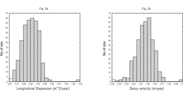
Figure 2 shows the two parameters Darcy flow and hydrodynamic dispersion as separate histograms. Figure 3 is a scatter plot that illustrates how the hydrodynamic dispersion (longitudinal dispersion) is related to the groundwater flow rate (Darcy velocity) and Figure 4 is a bivariate histogram of these two parameters, representing their joint pdf.

(16)

Figure 1 Plotting the Darcy velocity and the dispersion length data for the cases with

different variations used in Site-94 shows the general relationship between these parameters as used from that exercise. The straight line shows the result of a linear regression shown on a log-scale.

Figure 2 Histograms of longitudinal dispersion and Darcy velocity obtained by

applying the Discrete Feature Model to Site-94 data.

Dispersion Length (m**2/yr)

Darcy (m/yr) -5,5 -5,0 -4,5 -4,0 -3,5 -3,0 -2,5 -2,0 -1,5 -1,0 -0,5 0,0 0 1 2 3 4 5 6 7 8 9 Fig. 2b

Darcy velocity (m/year)

No of obs 0 5 10 15 20 25 30 35 40 45 50 55 60 65 70 75 -2,62 -2,43 -2,23 -2,04 -1,85 -1,66 -1,46 -1,27 -1,08 -0,89 -0,69 Fig. 2a

Longitudinal Dispersion (m**2/year)

No of obs 0 5 10 15 20 25 30 35 40 45 50 55 60 65 70 3,67 4,14 4,60 5,06 5,52 5,99 6,45 6,91 7,38 7,84 8,30

(17)

Figure 3 The relationship between the Darcy velocity and the dispersion length for the

data corresponding to the histograms of Figure 2. The straight line shows the result of a linear regression shown on a log-log scale.

Figure 4 The bivariate histogram of the Darcy velocity versus the dispersion on a

log-log scale, for the data corresponding to the diagram in figure 3.

Bivariate Histogram Empiric data - 406 samples

Longitudinal dispersion (m**2/year)

Darcy velocity (m/year)

-5,2 -4,8 -4,4 -4,0 -3,6 -3,2 -2,8 -2,4 -2,0 -1,6 -1,2 -0,8 -0,4 0,0 0 1 2 3 4 5 6 7 8 9 Correlation = 0.77

(18)

Hydrogeological calculations are usually separate from transport calculations in Monte Carlo studies of radionuclide transport in the geosphere because otherwise the

computational burden would be overwhelming. The results from hydrogeological simulations are obtained from 2 or 3D modelling, whereas the transport models are, in general, 1D. This poses the question of how to couple the two models, i.e., of how to transfer the data for use in the Monte Carlo calculations of the probabilistic assessment. In the stochastic calculations, the results of which are used in this work, 406 batches of particles were obtained at the surface, giving 406 pairs of values for the Darcy velocity and longitudinal dispersion. To use this data in the Monte Carlo calculations of

radionuclide transport it is usual to take the mean and standard deviations of the values for the Darcy velocities and the longitudinal dispersion (406 values for each in our case) and use them to characterise the central values of the probability distributions for the two parameters. In general, these distributions are assumed to be log-uniform or perhaps uniform. When performing the Monte Carlo calculations, one samples the parameter values for use in the geosphere transport model from these probability distributions, which are assumed to be independent from each other.

The above-described indirect method will not be used in this report other than for the purpose of comparing this approach to the direct approach which we claim should be used. The reason is this: in the direct approach we use as much of the information from the hydrogeological calculations as possible and, in particular, we do not disregard the eventual influence of a correlation existing between groundwater flow and dispersion that would be contained in the hydrogeological data. In the direct approach we use the values of the Darcy flow and longitudinal dispersion obtained directly from the discrete feature model, as input data to the geosphere model CRYSTAL (Robinson and Worgan, 1992) embedded in the SYVAC/SU Monte Carlo driver. This is possible because SYVAC/SU allows one to introduce data for the distributions through an input matrix, a feature include by Sundström in the last version of SYVAC/SU [8].

One question that immediately arises is how to obtain adequate statistics for the Monte Carlo calculations. One should consider that although 406 samples may be sufficient for the stochastic calculations made, using the discrete feature model (a balance between needs and computational burden posed by that 3D model) this may be too few samples for the Monte Carlo calculations. In fact, in these calculations one may vary a large number of parameters hence there is a need for a higher number of realisations. In this report we have monitored the convergence of the mean value of the peak release rate independent of time to control the statistics of the calculations. Furthermore, we have also introduced a procedure that obtains an arbitrary number of samples from a fitted distribution to the 3D histogram of Darcy flow versus longitudinal dispersion shown in Figure 4. In this way we also keep the correlation structure between those two

parameters. Appendix III includes a listing of the MatLab program developed for this direct approach.

(19)

3. Nuclides and input data

3.1 Nuclides included in the calculations

In this report, five nuclides are examined: carbon (14C), chlorine (36Cl), caesium (135Cs),

iodine (129I) and radium (226Ra). These nuclides are amongst those that contribute

substantially during the first 10 000 years to the intermediate dose potential (IDP) of the near-field for the Zero Variant case (A3) which is the reference case (see the figure on page 554, Vol. II of the SITE-94 report). For the same time period, these same nuclides are also some of the most important contributors to the flux from the far-field for the integrated Zero Variant calculation case in SITE-94 (see the figure on page 587, Vol.II of SITE-94 report). Hence, the choice of these radionuclides for our study.

3.2 Near-field data

The near-field breakthrough curves for each of the nuclides examined are used as the input for the far-field calculations. These curves were taken from the Reference Case, Zero Variant (A3) of SITE-94. For these calculations, it is conservatively assumed that the canister totally fails at a given time point (after 1000 years) , i.e., the whole fuel surface is in immediate and direct contact with the surrounding water from that moment on.

It is most probable that the chlorine, iodine, caesium and radium do not contribute to any solid phase formation. Carbon solubility might eventually be limited by isotope

exchange with calcite; nevertheless, solubility limits were consideredin the near-field

calculations, leading to the source term shown in Figure 5. Radium-226 is a decay product of the U-238 decay chain and exists in the fuel matrix as long as U-238. Its dissolution rate is therefore controlled by the congruent dissolution of the fuel matrix. Reducing conditions are assumed everywhere except on the surface of the fuel. Observe that for each nuclide we use one and the same near-field breakthrough curve, i.e., no Monte Carlo calculations are made for the near-field. The reason for this is that we are only interested in the implications of uncertainties associated with the

hydrogeological, physical and chemical evolution of the far-field.

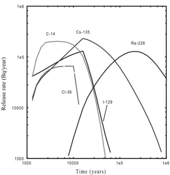
The near-field breakthrough curves mentioned above are shown in Figure 5. They were obtained from the CALIBRE model (Worgan and Robinson, 1995) (Appendix I). Details of the near-field calculations are not provided here. The interested reader should consult Volume II of the Site-94 report (SKI, 1996) for information on the input data and for the assumptions used in the near-field calculations.

The breakthrough curve for C-14 presented in Figure 5 corresponds to near-field releases from the fuel grain boundaries, the gap release and the release of carbon congruent with matrix dissolution.

(20)

Figure 5 Near-field breakthrough curves used as the source term for geosphere

transport calculations.

3.3 Far-field data

The Monte Carlo approach is used for the calculations of radionuclide transport in the geosphere. These transport calculations of the selected nuclides are made by keeping some parameters fixed and using probability distributions (pdfs) for others. Parameters other than the groundwater velocity and the longitudinal dispersion are sampled when needed using the simple Monte Carlo technique. The calculations take account of the fact that the groundwater flow and the hydrodynamic dispersion are correlated to each other, requiring the use of a joint distribution for these two parameters. Hence the pdf used here is a bivariate distribution from which the Darcy velocity and the longitudinal dispersion are sampled. This situation is in contrast to the commonly made assumption in Monte Carlo calculations that these two parameters are independent of each other and, as such, can be sampled from independent probability distributions. The

consequences of this situation will be analysed in detail.

To be able to compare the impact of using as much of the information output from the hydrogeological calculations as possible in the Monte Carlo simulations of far-field transport, we need to introduce two concepts that are implicit to the method chosen in this work by asking the following question:

• Is the hydrogeological data sufficient for the purpose of the Monte Carlo transport

Time (years)

Release rate (Bq/year)

1000 10000 1e5 1e6 1000 10000 1e5 1e6 I-129 Cs-135 Cl-36 C-14 Ra-226

(21)

could be assumed to form a complete set of data if one does not intend to vary other parameters in performing the Monte Carlo calculations of radionuclide transport, because, in this case, those points cover the parameter space very well. This can be checked easily by increasing the number of simulations from 406 to, say, 2030, i.e., by a factor of five. If the statistics of our original data set containing 406 pairs of points is complete, the output pdf obtained with the increased number of input points should be roughly the same as that resulting from the original 406 data pairs. The question then is how to extract reliable data to extend the number of realisations by a factor of five considering that we have only those 406 data points for the Darcy flow and the hydrodynamic dispersion. We will come back to this point later on.

On the other hand, if we want to vary not only the two flow parameters, but also several other parameters in our Monte Carlo calculations of radionuclide transport, the input parameter space covered by a total of 406 sampling points for each parameter entering in the Monte Carlo calculations may not be sufficient, although the information

regarding the two water-flow parameters themselves is complete. This depends on the number of parameters to be varied simultaneously as can be easily illustrated by the following example: suppose that we want to perform a Monte Carlo calculation where 10 parameters vary simultaneously, two of which are the two key flow parameters, the Darcy velocity and the hydrodynamic dispersion. If each parameter takes only three possible values, the minimum, the median and the maximum value of the pdf, then we

would need 103 realisations instead of 406 to obtain the total number of possible

combinations between those 10 parameters, or, for the general case, np realisations

where n is the number of parameters and p is the number of sampled points per

parameter. Looking at our original data given by the histograms displayed in Figure 2, we realise that using three points to characterise each pdf is far from enough. At the very least, one should include two more points, the upper and lower quartiles of the

distributions, for instance, but this would already necessitate 105 samples! In general,

however, so many samples are not needed. Nevertheless, to obtain good statistics from all the Monte Carlo calculations with more than two or three variable parameters, it is required that we sample quite a large number of parameter values while retaining the marginal correlations of the original joint pdf (or of its histogram). The way we achieve this with the empirical data set of 406 pairs of points as a starting point for the sampling procedure was described earlier.

Case studies

The issue of completeness and sufficiency leads us to the following set of calculations: • Variation calculations where the flow parameters obtained from the hydrogeology

calculations are the only ones to be varied.

• Variation calculations where the flow and transport parameters vary simultaneously These two sets unfold into the following groups of Monte Carlo calculations:

- Monte Carlo calculations with the original set of flow data, this data is a correlated

data set (Sections 4.1 and 5.1)

- Monte Carlo calculations with the original set of flow data, but treating the two

(22)

For the second set we have also done Monte Carlo calculations with the number of samples an order of magnitude higher, but using the correlated flow data set (Appendix II).

The flow parameters varying in the Monte Carlo calculations are given directly from the results of hydrogeological modelling using the Discrete Feature Model (Geier, 1996).

(23)

4. The impact of the spatial variability of flow

parameters

In the probabilistic calculations performed for this work, the random Monte Carlo sampling method is used as the only sampling strategy. Nevertheless, if we are stringent, we should not use the term random Monte Carlo calculations for the set of computations described in Section 4.1 because the only parameters that are varied are the Darcy velocity and the longitudinal dispersion, which are not independent of each other and are not sampled from distributions generated by random Monte Carlo sampling. In fact, they are extracted from an empirical distribution formed by unique and fixed values (not random values) extracted from hydrogeological modelling. It is in the hydrogeological modelling that one uses the field data as an input to calculate the groundwater flow in the geosphere. From the results of this modelling, one extracts the values of the Darcy flow and the hydrodynamic dispersion that form our empirical distribution for use in transport modelling of radionuclides in the far-field. As mentioned before, this two-step approach in which we decouple the flow modelling from the transport modelling is commonly used in probabilistic assessments to reduce the computational burden of the calculations.

4.1 Monte Carlo calculations with correlated input data

The data related to the two flow parameters, the Darcy velocity and the longitudinal dispersion is shown in Table I. This data gives the central values of the marginals of the empirical or joint distribution used in the calculations. In Table II this pdf is labelled “empirical”. The groundwater flow rate (the Darcy flow) varies by two orders of magnitude and hydrodynamic dispersion by five orders of magnitude. The marginal distribution of the Darcy flow has the shape shown in Figure 2b, while the marginal pdf of the hydrodynamic dispersion is shown in Figure 2a.

Table II presents the nuclides studied in this work and a summary of the far-field para-meters needed in this section for use in the geosphere transport model CRYSTAL.

Table I Central values for the marginal distributions of the joint

pdf given in Table II.

Parameter Darcy flow Hydrodynamic dispersion

Mean 2.22 x 10-2 _{1.18 x 10}6 Confid. (-95%) 2.06 x 10-2 0.0 Confid. (+95%) 2.38 x 10-2 _{2.55 x 10}6 Median 1.99 x 10-2 _{1.17 x 10}5 Minimum 2.41 x 10-3 _{4.72 x 10}3 Maximum 2.02 x 10-1 2.00 x 108 Lower Quart. 1.35 x 10-2 _{4.82 x 10}4 Upper Quart. 2.71 x 10-2 _{2.70 x 10}5 Variance 2.62 x 10-4 _{1.96 x 10}14 Std. Dev. 1.62 x 10-2 _{1.40 x 10}7 Skewness 6.46 x 100 _{1.42 x 10}1

(24)

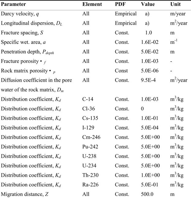
Table II Far-field parameters values for the constant parameters.

Parameter Element PDF Value Unit

Darcy velocity, q All Empirical a) m/year

Longitudinal dispersion, DL All Empirical a) m2/year

Fracture spacing, S All Const. 1.0 m

Specific wet. area, a All Const. 1.6E-02 m-1

Penetration depth, Pdepth All Const. 5.0E-02 m

Fracture porosity • f All Const. 1.0E-03

-Rock matrix porosity • p All Const 5.0E-06

-Diffusion coefficient in the pore

water of the rock matrix, Dm

All Const. 9.5E-4 m2/year

Distribution coefficient, Kd C-14 Const. 1.0E-03 m3/kg

Distribution coefficient, Kd Cl-36 Const. 0 m3/kg

Distribution coefficient, Kd Cs-135 Const. 1.0E-01 m3/kg

Distribution coefficient, Kd I-129 Const. 5.0E-04 m3/kg

Distribution coefficient, Kd Cm-246 Const. 5.0E+00 m3/kg

Distribution coefficient, Kd Pu-242 Const. 5.0E+00 m3/kg

Distribution coefficient, Kd U-238 Const. 5.0E+00 m3/kg

Distribution coefficient, Kd U-234 Const. 5.0E+00 m3/kg

Distribution coefficient, Kd Th-230 Const. 1.0E+00 m3/kg

Distribution coefficient, Kd Ra-226 Const. 5.0E-01 m3/kg

Migration distance, Z All Const. 500.0 m

(25)

4.1.1 Results and Uncertainty Analysis

In this section we present the results of the radionuclide transport calculations and an uncertainty analysis of these results. All results refer to calculations of radionuclide migration escaping from one single canister. Because modelling biosphere transport is not within the scope of this work, the outcomes of the transport calculations refer only to the far-field and therefore the results and the corresponding analysis are expressed in units of Becquerel and not in Sievert.

The measures of importance for the present analysis are based on the release rate of radionuclides independent of time.

Carbon-14 migration

The release rate of C-14 independent of time is shown in Fig. 6. This distribution shows that the uncertainty is small.

Figure 6 The far-field histogram for C-14release. Three decimals are needed in this histogram because of the very low uncertainty of the peak release distribution.

Caesium-135 migration

The release rate of Cs-135 independent of time is shown in Figure 7. This distribution is left skewed as are the distributions for the remaining nuclides shown in Figures 8 to 10.

Release rate independent of time (Bq/year)

No of obs 0 10 20 30 40 50 60 70 80 90 100 110 120 130 140 150 5,372 5,374 5,376 5,379 5,381 5,383 5,385 5,387 5,389 5,391 5,394

(26)

Figure 7 The far-field histogram for caesium release. Cl-36 migration

The release of Cl-36 is in the form of a pulse shape with a lower level tail. This shape results from the fact that Cl-36 is highly mobile with a nil sorption coefficient.

Figure 8 The far-field histogram for Cl-36.

Release rate independent of time (B/year)

No of obs 0 14 28 42 56 70 84 98 112 126 140 154 168 182 196 210 <= 4,81687 4,81698 4,81709 4,81719 4,81730 4,81740 4,81750

No of obs 0 8 16 24 32 40 48 56 64 72 80 88 96 104 112 120 5,22 5,23 5,24 5,26 5,27 5,29 5,30 5,32 5,33 5,35 5,36

(27)

I-129 migration

Iodine displays an output distribution that is not as skewedas that of Cl-36. A finite but

small distribution coefficient (Kd = 5.0E-04 m3/kg) was assumed for the sorption of

iodine, which is in contrast with chlorine with a nil Kd value.

Figure 9 The far-field histogram for iodine.

Ra-226 migration

Figure 10 The far-field histogram for Ra-226 from the decay chain.

No of obs 0 5 10 15 20 25 30 35 40 45 50 55 60 65 70 75 5,11275 5,11293 5,11311 5,11329 5,11348 5,11366

No of obs. 0 8 16 24 32 40 48 56 64 72 80 88 96 104 112 120 4,46 4,53 4,59 4,66 4,72 4,78 4,85 4,91 4,98 5,04 5,11

(28)

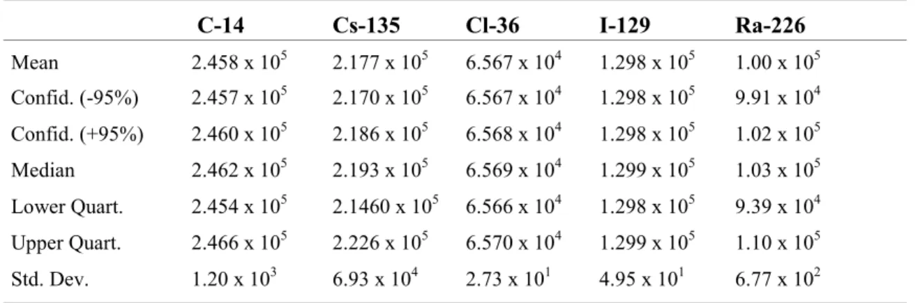
The calculations for all nuclides show an unusually low uncertainty as it is clearly displayed in Table III.

Table III Central values of peak releases for all nuclides.

C-14 Cs-135 Cl-36 I-129 Ra-226 Mean 2.458 x 105 _{2.177 x 10}5 _{6.567 x 10}4 _{1.298 x 10}5 _{1.00 x 10}5 Confid. (-95%) 2.457 x 105 _{2.170 x 10}5 _{6.567 x 10}4 _{1.298 x 10}5 _{9.91 x 10}4 Confid. (+95%) 2.460 x 105 _{2.186 x 10}5 _{6.568 x 10}4 _{1.298 x 10}5 _{1.02 x 10}5 Median 2.462 x 105 _{2.193 x 10}5 _{6.569 x 10}4 _{1.299 x 10}5 _{1.03 x 10}5 Lower Quart. 2.454 x 105 _{2.1460 x 10}5 _{6.566 x 10}4 _{1.298 x 10}5 _{9.39 x 10}4 Upper Quart. 2.466 x 105 _{2.226 x 10}5 _{6.570 x 10}4 _{1.299 x 10}5 _{1.10 x 10}5 Std. Dev. 1.20 x 103 _{6.93 x 10}4 _{2.73 x 10}1 _{4.95 x 10}1 _{6.77 x 10}2

The parameters that are varied in the simulations are the two flow parameters Darcy flow and hydrodynamic dispersion. The Darcy flow has an uncertainty of two orders of magnitude and the hydrodynamic dispersion varies by almost five orders of magnitude. Yet the propagation of these uncertainties does not result in a wide uncertainty in the maximum release rate independent of time. The explanation for this observation is given by the sensitivity analysis done in Section 5.

The mean value of the maximum release rate (peak release) for the Monte Carlo calculations of all nuclides using 406 samples is expected to have converged because we vary only two parameters. A curve illustrating the mean peak as a function of the number of samples is shown in Figure 11 for caesium. A sudden jump is observed at around 200 samples, it is caused by the inclusion of an “extreme” parameter value when the number of samples goes from 200 to 250 samples. In fact it is a small percentage increase. When we increase the number of variable parameters by including random variations of other flow parameters and of transport parameters, the convergence of the Monte Carlo calculations should be carefully considered.

4.1.2 Sensitivity Analysis

As the calculations performed in this section only deal with two variable parameters, the Darcy velocity and the longitudinal dispersion, one could anticipate a straightforward sensitivity analysis. Unfortunately this is not the case, which has been the motivation for

pursuing this analysis.

(29)

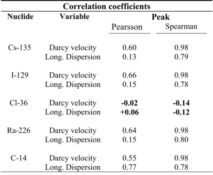
Figure 11 The variation in the peak release of 135Cs with number of samples. The results computed with the help of the approaches mentioned above are shown in Table IV. Both methods identify the Darcy velocity as the most important parameter. Qualitatively they are also consistent in the sense that in each case an increase in the Darcy velocity implies an increase in the peak release rate; the same prediction is made for increasing values of the longitudinal dispersion. The results of the Spearman test for caesium and iodine are consistent with other non-parametric tests (Kendall and Gamma tests), the results of which we do not include here. For all non-parametric tests the numerical values are relatively close: the Darcy velocity shows a correlation with the peak release which varies between 0.91 and 0.98 and the longitudinal dispersion coefficient varies between 0.60 and 0.79. The Spearman test is “less” non-parametric than the Kendall and Gamma tests.

Table IV Sensitivities of peak release for the two correlated flow parameters.

Correlation coefficients

Nuclide Variable Peak

Pearsson Spearman Darcy velocity 0.60 0.98 Cs-135 Long. Dispersion 0.13 0.79 Darcy velocity 0.66 0.98 I-129 Long. Dispersion 0.15 0.78 Cl-36 Darcy velocity -0.02 -0.14 Long. Dispersion +0.06 -0.12

Ra-226 Darcy velocity 0.64 0.98

Long. Dispersion 0.15 0.80

C-14 Darcy velocity 0.55 0.98

Long. Dispersion 0.77 0.78

Number of samples

Peak mean value (B/year)

2,14e5 2,16e5 2,18e5 2,2e5 2,22e5 2,24e5 2,26e5 0 50 100 150 200 250 300 350 400 450 Cesium-137

(30)

The quantitative predictions vary strongly between the Pearsson correlation and the Spearman test. Observe however that one cannot expect the same absolute numerical values from different tests, so when we talk about a strong variation in the results, we refer to the relative difference between the numerical values for the two parameters within each test. For example, for Cs-135 the Pearsson test puts the Darcy velocity as the first parameter, it also tells us that it is much more important than the longitudinal dispersion (0.60 against 0.13 respectively). Recalling our previous knowledge that these two parameters, which come from hydrogeological information, are strongly correlated (linear correlation of 0.71), it seems clear that one or both methods break down in the presence of correlations between the pdf of the parameters. Figure 12 shows clearly the impact of these correlations on the peak release. Any horizontal slice at any Z=constant value, displays the elliptical correlation pattern shown in the scatter plot for these two parameters in Figure 3. The most striking result is the complete breakdown of the two statistical methods for the results of the Cl-36 migration. The reason is the very small uncertainty associated with the strong low release tail of the distribution for Cl-36 (Figure 8).

Figure 12 The relation between the variable parameters and the peak release of

Cs-135. The graph shows clearly the correlation between both parameters and the impact of these parameters on the release.

1,582e5 1,664e5 1,745e5 1,827e5 1,909e5 1,991e5 2,073e5 2,155e5 2,236e5 2,318e5 above Cs-135

(31)

between the two flow parameters. It is difficult at present to know which method best represents the truth.

The methods described above are correlation methods. Recently developed sensitivity methods based on variance, for instance the Sobol indices (Sobol, 1993) and Fourier Amplitude Sensitivity (Saltelli and Bolado, 1998), can compute higher-order terms for sensitivity indices and total indices whenever the results are non-linear functions of the input parameters, but unfortunately they cannot handle the case of correlated

parameters. In summary, even when applied to the apparently simple case of two varying parameters that are correlated, the methods used in this section and other methods can only give us qualitative results.

4.2 Monte Carlo calculations with uncorrelated input data

The approach suggested in this report to reduce the hydrogeological data to the format needed by the transport models conserves the correlation structure of the data. In the calculations made in this report only two parameters appear as correlated data: the Darcy flow and the longitudinal dispersion. The immediate question is therefore: what is the impact of this correlation on the results of the transport models.

The straightforward way to answer to this question is to “decorrelate” those parameters and repeat the calculations in order to compare with the results obtained in Section 4.1. This “decorrelation” is made by random mixing of the data. If X1(N) is a vector

containing the Darcy parameter values and X2(N) the one containing the longitudinal dispersion values (with N=406 realisations in our case), we can take each of them separately and perform a random permutation of their values. After this operation the correlation values between the Darcy and the longitudinal dispersion values is nil.

4.2.1 Results and Uncertainty Analysis

The scatter plot of Figure 13 shows the flow field data used in the Monte Carlo

calculations. In this figure one can see a region with a structure that is non-random. The original pattern obtained by the permutation is perfectly random, but some of the pairs

of values for the Darcy velocity q, and the longitudinal dispersion DLresult in Peclet

numbers higher than 100 which cannot be handled by the CRYSTAL model used in the transport calculations. The Peclet number is defined by:

where q [m/year] is the Darcy velocity, L [m] is the transport length, • [-] is the flow

porosity and DL [m2/year] is the longitudinal dispersion coefficient. Physically the

Peclet number is the ratio of the dispersive over the convective (or advective) term in the transport equation.

L

D qL

(32)

Figure 13 Scatter plot of Darcy velocity versus longitudinal dispersion parameters.

The graph shows that the parameters are "decorrelated". The special linear structure at the bottom of the picture results from resetting with unphysical pairs of data (see text). What has been done to tackle this situation was to reset the longitudinal dispersion values leading to Peclet numbers that are greater than 100 to the highest value compatible with a Peclet number equal to 100. In this way one can avoid physically unreasonable combinations of parameters. Although some combinations of Darcy values with longitudinal dispersion values such that the Peclet is higher than 100 could be physically reasonable, the difference in the output consequences is insignificant. In this section an uncertainty analysis is done with the same input data for the Monte Carlo calculations as that used in Section 4.1.1 with the exception of the

hydrogeological parameters Darcy flow and longitudinal dispersion, which are those obtained from the original data set after decorrelation.

The results obtained with this new input data are presented in Table V and as

histograms (Figure 14). Comparing these results with those of Table III for the case of correlated flow data, it is observed that the correlation has no impact on the mean values of the peak release rates for any nuclide. This is not always the case. For instance, Pereira (Pereira and Sundström, 2000) found a discrepancy of half an order of magnitude for the mean peak release in Monte Carlo calculations between correlated and non-correlated data.

The results obtained in Table V are as expected. In fact, in the situation modelled here the geosphere has an extremely low impact on the attenuation of the mean peak releases as is clearly illustrated by Figure 15. In this figure, we have plotted the near-field curve of Cs-135 together with the ten breakthrough curves, which have the highest peak releases for the simulated nuclide. These ten curves dominate over the mean peak values. We see that in every case considered here the peak of the far-field curves is

Scatterplot of decorrelated flow parameters

Darcy velocity (m/year) Longitudinal dispersion (m**2/year) ₁₀₀₀₀

1e5 1e6 1e7 1e8

(33)

expected that the sensitivity indices obtained in the sensitivity analyses of the correlated and uncorrelated data will be almost the same (see next section). The impact of the correlations on the pdfs at different points in time will be examined later on.

Figure 14 The histograms of peak release rates for random sampling of the flow

parameters.

Histogram of Cs-135: random sampling

Peak release rate (Bq/year)

No of obs 0 6 12 18 24 30 36 42 48 54 60 66 72 78 84 90 5,22 5,23 5,25 5,26 5,27 5,29 5,30 5,32 5,33 5,34 5,36

Histogram of I-129: random sampling

Peak release (Bq/year)

No of obs 0 6 12 18 24 30 36 42 48 54 60 66 72 78 84 5,1126 5,1128 5,1130 5,1131 5,1133 5,1135 5,1136 5,1138

Histogram of Ra-226: random sampling

No of obs 0 8 16 24 32 40 48 56 64 72 80 88 96 104 112 4,64 4,69 4,74 4,78 4,83 4,87 4,92 4,97 5,01 5,06 5,11

Cl-36, random flow parameters

No of obs 0 13 26 39 52 65 78 91 104 117 130 143 156 169 182 195 4,8167 4,8168 4,8170 4,8171 4,8172 4,8173 4,8175

Histogram of C-14: random sampling

No of obs 0 8 16 24 32 40 48 56 64 72 80 88 96 104 112 120 5,372 5,374 5,377 5,379 5,381 5,383 5,386 5,388 5,390 5,393

(34)

Table V Central values for all nuclides for uncorrelated parameters. C-14 Cs-135 Cl-36 I-129 Ra-226 Mean 2.460 x 105 2.185 x 105 6.570 x 104 1.300 x 105 1.021 x 105 Confid. (-95%) 2.459 x 105 _{2.179 x 10}5 _{6.568 x 10}4 _{1.298 x 10}5 _{1.010 x 10}5 Confid. (+95%) 2.461 x 105 _{2.190 x 10}5 _{6.568 x 10}4 _{1.299 x 10}5 _{1.032 x 10}5 Median 2.462 x 105 _{2.197 x 10}5 _{6.565 x 10}4 _{1.299 x 10}5 _{1.042 x 10}5 Lower Quart. 2.456 x 105 _{2.152 x 10}5 _{6.570 x 10}4 _{1.298 x 10}5 _{9.604 x 10}5 Upper Quart. 2.466 x 105 _{2.223 x 10}5 _{6.570 x 10}4 _{1.299 x 10}5 _{1.094 x 10}5 Std. Dev. 9.560 x 102 _{5.680 x 10}3 _{3.040 x 10}1 _{4.280 x 10}1 _{1.130 x 10}4

Figure 15 The relation between near-field and some far-field breakthrough curves for

Cs-135.

4.2.2 Sensitivity Analysis

The sensitivity analysis conducted here uses three non-parametric methods and one parametric one (the Pearsson correlation coefficients). The results are summarised in

Far-field release for 10 breakthrough curves

Time (years)

Release rate (Bq/yr)

0 40000 80000 1,2e5 1,6e5 2e5 2,4e5

0 2e5 4e5 6e5 8e5 1e6

Near-field (Cesium)

Time (years)

0 40000 80000 1,2e5 1,6e5 2e5 2,4e5

(35)

methods is approximately the same, which was not the case for the calculations performed with correlated parameters.

Table VI Sensitivity values for uncorrelated data.

Correlation coefficients for uncorrelated flow parameters

Nuclide Variable _Peak

Pearsson Spearman Kendal Gamma

Darcy velocity 0.61 0.94 0.83 0.83

Cs-135

Long. Dispersion 0.14 0.22 0.15 0.15

I-129 Darcy velocity 0.65 0.94 0.83 0.84

Long. Dispersion 0.16 0.22 0.15 0.14

C-14 Darcy velocity 0.55 0.94 0.83 0.83

Long. Dispersion 0.11 0.21 0.15 0.15

Cl-36 Darcy velocity 0.04 -0.07 0.0 -0.01

Long. Dispersion 0.06 -0.07 -0.05 -0.06

Ra-226 Darcy velocity 0.62 0.93 0.81 0.81

Long. Dispersion 0.17 0.25 0.17 0.17

This indicates that the rank method is somewhat more sensitive to the presence of correlations as shown in Table IV.

Furthermore for these Monte Carlo calculations with uncorrelated parameters, the sensitivity analysis methods break down for the Cl-36 radionuclide migration. This result was also found for similar calculations in which the parameters were correlated; hence, the fact that the parameters are correlated is not the explanation for the failure.

(36)

(37)

5. The impact of flow and transport parameter

uncertainties

5.1 Monte Carlo calculations with correlated input data

In Section 4 it was demonstrated that although input data varied by at least two orders of magnitude, the two flow parameters, Darcy velocity and longitudinal dispersion, did not have an impact on the uncertainty in the peak release rates, the pdf of this distribution having a very low standard deviation. The explanation for this is that the transport parameters were kept constant during the Monte Carlo simulations.

In this section we organise the calculations in the following way: first, we make some exploratory calculations on Cs-135 in which we systematically increase the number of variable parameters from calculation to calculation. The results are shown in Appendix II. Second, we make radionuclide transport calculations for all nuclides, but now varying all parameters simultaneously.

The goal of the first set of exploratory calculations was to illustrate how the uncertainty in the flow and transport parameters propagates through the models for each new parameter that we allow to vary. These calculations resulted in a considerable

broadening of the distribution representing the consequences that would be observed. Hence, the small uncertainty observed originally in the propagation of the two

hydrogeological parameters, the advective velocity and the longitudinal dispersion is masked in the final results of these calculations.

The goal of the second set of calculations was to examine the impact of the uncertainty in the parameters for all nuclides considering that the hydrogeological data representing the Darcy velocity and the longitudinal dispersion are correlated.

5.1.1 Results and uncertainty analysis

In the set of calculations used in this section, the parameters that are considered to be uncertain for each nuclide are varied simultaneously. The input data for all parameters is displayed in Table VII. The variable parameters are sampled within certain intervals taken from different sources. The boundaries of the distribution coefficients come from: Cl-36 – lower limit (Table 15.2.7), Site-94 report and upper limit, TVO-92 report; C-14 – lower limit, Site-94 report and upper limit data from fracture fillings SKI-TR: 96-2 pp. 7; Cs-135 – lower limit Site-94 report and upper limit chosen as a factor of the lower limit; I – lower limit Site-94 report and upper limit 2.3 times higher than low limit (less than for the oxidising case); Cm-246 – lower limit from Site-94 report and upper limit equal to the value of far-field rock given by SKI-TR:96-2, pp. 22; Pu-242 – lower limit from fracture filling III reducing conditions SKI-TR:96-2, pp.21 and upper limit from Site-94; U234 and 238 – lower limit from fracture filling III reducing conditions SKI-TR:96-2, pp.19 and upper limit from SITE-94 report; Th-230 – lower limit from fracture filling III reducing conditions, SKI-TR:96, pp.17 and upper limit from Site-94; Ra-226 – lower limit from TVO-92 report and upper limit from SITE-94 report.

(38)

The results are summarised in Table VIII and by the histograms of Figure 16. The probabilistic results of the uncertainty analysis are presented in Fig 17 where they are

given by the mean value of the peak releases and confidence levels of ±95%. In the

logarithmic scale, the confidence intervals lie very close to the respective mean values. The deterministic results of SITE-94 data (Table 16.3.4, Vol. II) are shown in the same figure. One can observe that the deterministic maximum releases of C-14 and I-129 according to the data from SITE-94 are near the mean values of the peak releases of the probabilistic calculations. For Cl-36 the deterministic results differ by one order of magnitude and for Cs-135 and Ra-226, the discrepancy is higher than one and two orders of magnitude, respectively. But one should consider that the parameter variations in the probabilistic calculations not only cover the integrated "Zero Variant" case for the "Reference Case" of the SITE-94 study, but also other more conservative cases given in the SITE-94 report.

Histogram of Cs-135 Correlated flow parameters

No of obs 0 5 10 15 20 25 30 35 40 45 50 55 60 65 3,01 3,24 3,46 3,69 3,92 4,14 4,37 4,60 4,82 5,05 5,28 Histogram of Cl-36 Correlated flow parameters

No of obs 0 23 46 69 92 115 138 161 184 207 230 253 276 299 322 345 4,804 4,805 4,807 4,808 4,809 4,811 4,812 4,813 4,815 4,816 4,818 Histogram of I-129 Correlate flow parameters

No of obs 0 20 40 60 80 100 120 140 160 180 200 220 240 260 280 300 4,92 4,94 4,96 4,98 5,00 5,02 5,04 5,05 5,07 5,09 5,11 Histogram of Ra-226 Correlated flow parameters

No of obs 4 8 12 16 20 24 28 32 36 40 44 48 Histogram of C-14

Correlated flow parameters

No of obs 0 10 20 30 40 50 60 70 80 90 100 110 120 130 140 150 3,22 3,44 3,65 3,87 4,09 4,31 4,52 4,74 4,96 5,18 5,39

(39)

Table VII Parameters and distributions used in the calculations.

Parameter Element PDF Value Unit

Darcy velocity, q All Empirical a) m/year

Longitudinal dispersion, DL All Empirical a) m2/year

Fracture spacing, S All Const. 1.0 m

Specific wet. area, a All Uniform 6.3E-03 7.86E-01 1/m

Penetration depth, Pdepth All Uniform 2.0E-02 2.50E-01 m

Fracture porosity • f All Const. 1.0E-03

-Rock matrix porosity • p All Const 5.0E-06

-Diffusion coefficient in the pore

water of the rock matrix, Dm

All Const. 9.5E-4 m2/year

Distribution coefficient, Kd C-14 Uniform. 1.0D-3 1.0D-2 m3/kg

Distribution coefficient, Kd Cl-36 Uniform 0.0 1.0D-4 m3/kg

Distribution coefficient, Kd Cs-135 Uniform 1.0E-01 5.0E-01 m3/kg

Distribution coefficient, Kd I-129 Uniform 3.0E-04 7.0E-04 m3/kg

Distribution coefficient, Kd Cm-246 Uniform 0.0 5.0 m3/kg

Distribution coefficient, Kd Pu-242 Uniform 2.0 5.0 m3/kg

Distribution coefficient, Kd U-238 Uniform 1.0 5.0 m3/kg

Distribution coefficient, Kd U-234 Uniform 1.0 5.0 m3/kg

Distribution coefficient, Kd Th-230 Uniform 0.1 1.0 m3/kg

Distribution coefficient, Kd Ra-226 Uniform 0.2 0.5 m3/kg

Migration distance, Z All Const. 500.0 m

a) data given by the empirical distribution (joint pdf) shown in Fig. 4.

Table VIII Central values for all nuclides†_.

C-14 Cs-135 Cl-36 I-129 Ra-226 Mean 1.583 x 105 _{9.406 x 10}4 _{6.562 x 10}4 _{1.267 x 10}5 _{2.271 x 10}4 Confid. (-95%) 1.527 x 105 _{8.850 x 10}4 _{6.561 x 10}4 _{1.261 x 10}5 _{2.001 x 10}4 Confid. (+95%) 1.639 x 105 _{9.961 x 10}4 _{6.563 x 10}4 _{1.272 x 10}5 _{2.542 x 10}4 Median 1.617 x 105 _{8.259 x 10}4 _{6.563 x 10}4 _{1.286 x 10}5 _{1.041 x 10}4 Lower Quart. 1.172 x 105 _{4.563 x 10}4 _{6.561 x 10}4 _{1.266 x 10}5 _{4.273 x 10}3 Upper Quart. 2.096 x 105 _{1.362 x 10}5 _{6.566 x 10}4 _{1.295 x 10}5 _{2.949 x 10}4 Std. Dev. 5.735 x 104 _{2.825 x 10}3 _{1.185 x 10}2 _{5.759 x 10}3 _{2.776 x 10}4

(40)

Figure 17 Deterministic results from SITE-94 (low F-ratio variation case) versus

probabilistic results from this work.

5.1.2 Sensitivity analysis

Statistical methods of global sensitivity analysis

In this section we perform the sensitivity analysis for output distributions in calculations in which five parameters were simultaneously varied: the Darcy velocity q, the

hydrodynamic or longitudinal dispersion DL, the flow wetted surface area a, the

penetration depth Pdepth and the distribution coefficient Kd. One should bear in mind,

that in general a sensitivity analysis is not as dependent on the number of samples as an uncertainty analysis. Obviously, if we have a relatively low number of simulations, the numerical results will not be as exact as if the convergence of the Monte Carlo

calculations had been fully attained by using a very high number of samples, but we can still get the general trends about the relative importance of the different parameters if we are not far away from a full convergence of the Monte Carlo calculations. It is the case here, as is shown by the rapidly decreasing oscillatory behaviour of the mean peak shown in Figure 18.

In this section we again use two methods of sensitivity analysis, the first based on the Deterministic results from SITE-94 versus probabilistisc results

Nuclide

4,0 4,4 4,8 5,2 5,6 6,0 6,4 Ra-226 Cs-135 Cl-36 C-14 I-129

Deterministic data from SITE-94 Mean, probabilistic data Conf. level -95% Conf. level +95%

(41)

For each nuclide we observe a general consistency between the results of the non-parametric test (Spearman) and the Pearsson correlation coefficient with one important exception: for all nuclides the Spearman correlation coefficient for the longitudinal dispersion parameter is very different from the Pearsson correlation coefficient. It is most likely that this disagreement arises because the Darcy flow is correlated to the longitudinal dispersion. It is not possible from the results to explain why the difference appears in the longitudinal dispersion parameter and not in the Darcy correlation parameter; in this respect there is also one exception, the Darcy correlation parameter for the iodine nuclide from the Pearsson statistics is quite different from that from the Spearman statistics.

Another interesting observation is related to the values of Cl-36 given by both statistics, which are generally lower for all parameters than the values for the other nuclides. This is probably caused by to the very low variance of the peak release associated with the skewness of its distribution.

Resuming our discussion of the results displayed in Table IX below, we observe that the wetted surface area a is the most important parameter for all nuclides apart from Cl-36 (for Pearsson statistics). The second most important parameter is the groundwater flow, the exceptions being for Cl-36 and I-129 (Pearsson statistics); in general the distribution coefficient is the third most important parameter according to Pearsson statistics

whereas this place is taken by the longitudinal dispersion according to the Spearman statistics. The penetration depth is important only for Cl-36 and I-129, which are the nuclides with very low distribution coefficients. This indicates that if these nuclides are retarded, it is because of the diffusion mechanism in the matrix, but without retention

due to a Kd -effect.

Cl-36 is the nuclide with lowest dispersion and that, which poses difficulties when subjecting the two sets of statistics to the sensitivity analysis. We have seen before that global sensitivity analysis breaks down totally for this nuclide when only the flow parameters are varying (Table IV).

(42)

34

tw

o correlated flow parameters. The intege

rs in bold represent the parameter rank.

Cs-135 C-14 Ra-226 Peak rel ease P eak rel ease. P eak rel ease. P earsson S pearm an P earsson S pearm an P earsson S pearm an 0.43 2 0.55 2 0.41 2 0.52 2 0.45 2 0.55 3 -0.18 3 -0.20 4 -0.27 3 -0.27 4 -0.10 4 -0.18 4 0.17 4 0.46 3 0.11 4 0.44 3 0.27 3 0.57 2 -0.001 5 -0.005 5 -0.06 5 -0.06 5 -0.03 5 -0.008 5 -0.80 1 -0.80 1 -0.74 1 -0.77 1 -0.71 1 -0.73 1 Cl -3 6 I-129 Peak rel ease P eak rel ease P earsson S pearm an P earsson S pearm an 0.15 4 0.16 4 0.29 3 0.46 2 -0.22 2 -0.20 3 -0.17 4 -0.18 5 0.05 5 0.16 4 0.04 5 0.39 3 -0.24 1 -0.21 2 -0.33 2 -0.37 4 -0.20 3 -0.31 1 -0.39 1 -0.71 1

(43)

Figure 18 The variation of the mean peak value of 135Cs with increasing number of samples. Five parameters are varied in this calculation. The oscillatory behaviour indicates that that the calculation is approaching convergence.

Finally we observe that in all cases there is an agreement on the type of impact that the different parameters of the input distributions have on the output distribution: the Darcy flow is positive, i.e., the higher this parameter is the higher is the peak release rate. The

distribution coefficient Kd has a negative correlation showing that the lower the Kd is,

the higher the peak release rate will be. The correlation value signals that the

penetration depth, Pdepth and the wetted surface are also in accordance with the physical

meanings of the parameters, although the two statistics do not work properly in the presence of the correlation between groundwater flow (Darcy velocity) and longitudinal dispersion.

The sensitivity of the consequences to the variation of the parameters can be visualised by “sensitivity plots” (figure 18). Qualitatively one can say that the greater the distance of the cumulative curve to the diagonal, the more sensitive is the parameter.

Cs-135

Number of samples

Mean peak (Bq/year)

86000 88000 90000 92000 94000 96000 98000 1e5 0 50 100 150 200 250 300 350 400 450