DOI:10.1051/0004-6361/201628768 c ESO 2017
Astronomy
&
Astrophysics
MCDHF and RCI calculations of energy levels, lifetimes
and transition rates for 3l3l
0
, 3l4l
0
, and 3s5l states
in Ca IX – As XXII and Kr XXV
?
S. Gustafsson
1, P. Jönsson
1, C. Froese Fischer
2, and I. P. Grant
3, 41 Group for Materials Science and Applied Mathematics, Malmö University, 211 19 Malmö, Sweden
e-mail: stefan.gustafsson@mah.se
2 National Institute of Standards and Technology, Gaithersburg, MD 20899, USA 3 Oxford University, Mathematical Institute, Oxford OX2 6GG, UK
4 Cambridge University, Department of Applied Mathematics and Theoretical Physics, Centre for Mathematical Sciences,
Cambridge CB3 0WA, UK
Received 22 April 2016/ Accepted 18 July 2016
ABSTRACT
Multiconfiguration Dirac-Hartree-Fock (MCDHF) calculations and relativistic configuration interaction (RCI) calculations were per-formed for states of the 3l3l0
, 3l4l0
and 3s5l configurations in the Mg-like ions Ca IX – As XXII and Kr XXV. Valence and core-valence electron correlation effects are accounted for through large configuration state function expansions. Calculated excitation energies are in very good agreement with observations for the lowest levels. For higher lying levels observations are often missing and present energies aid line identification in spectra. Lifetimes and transition data are given for all ions. There is an excellent agreement for both lifetimes and transition data with recent multiconfiguration Hartree-Fock Breit Pauli calculations.
Key words. atomic data – methods: numerical – line: identification
1. Introduction
Mg-like ions are of considerable interest for diagnostic purposes in astrophysical plasmas and in fusion plasmas. The background and diagnostic details are given inAggarwal et al.(2007) as well as in a series of comprehensive papers by Landi and Bhatia (Landi & Bhatia 2014;Bhatia & Landi 2011;Landi 2011).
During the past years a large number of calculations have been performed for Mg-like ions. In addition to the calcula-tions above, see for example, Safronova et al. (2000), Froese Fischer et al. (2006), Massacrier & Artru (2012), Hu et al. (2014),Si et al.(2015),Santana & Träbert(2015). The most re-cent R-matrix calculations for the Mg-like ions include both collisional and radiative data (Fernandez-Menchero et al. 2014). Some of the calculations above provided data only for levels in the n= 3 complex but, as pointed out byLandi(2011), the real need is for data involving configurations with n ≥ 4.
In addition to energies and transition data involving config-urations with n ≥ 4, there is also a need for transition ener-gies that are accurate enough to aid line identifications. To meet these needs, systematic large scale relativistic multiconfiguration calculations were performed for states belonging to the 3l3l0, 3l4l0and 3s5l0configurations in the ions Ca IX – As XXII and
Kr XXV. The present calculations provide a consistent and accu-rate data set for line identification and modeling purposes. The data set can also be used as a benchmark for other calculations.
? Tables for energy levels, lifetimes, and transition data and full
Tables 2, 4, and 6 are available at the CDS via anonymous ftp to
cdsarc.u-strasbg.fr(130.79.128.5) or via
http://cdsarc.u-strasbg.fr/viz-bin/qcat?J/A+A/597/A76
2. Relativistic multiconfiguration calculations The calculations were performed using the four-component fully relativistic multiconfiguration Dirac-Hartree-Fock (MCDHF) method relying on multireference single and double (MRSD) substitutions for generating wave function expansions. The method is described in detail in (Grant 2007) and in a recent re-view of multiconfiguration methods (Froese Fischer et al. 2016).
2.1. Multiconfiguration Dirac-Hartree-Fock
An atomic state is described by a wave functionΨ, that is a solu-tion to the wave equasolu-tion based on the Dirac-Coulomb Hamilto-nian. In the MCDHF method, the wave functionΨ(γPJM) for a state labeled γPJM with γ being the orbital occupancy and angu-lar coupling scheme, P the parity, and J and M the total anguangu-lar quantum numbers, is expanded in configuration state functions (CSFs) Ψ(γPJM) = NCSF X j=1 cjΦ(γjPJM). (1)
The CSFs are antisymmetrized and symmetry-adapted many electron functions built from products of one-electron Dirac or-bitals (Grant 2007;Froese Fischer et al. 2016).
The wave functions were determined in the extended optimal level (EOL) scheme and the radial parts of the Dirac orbitals and the expansion coefficients of the studied states were obtained it-eratively in a layer by layer approach, as specified in Sect. 2.3, from a set of equations that results from applying the variational
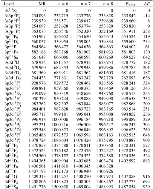
Table 1. Calculated excitation energies including low-frequency Breit and QED effects in cm−1for Fe XV as a function of the increasing size of
the CSF expansion.
Level MR n= 6 n= 7 n= 8 ENIST ∆E
3s2 1S0 0 0 0 0 0 0 3s3p3P◦ 0 234 093 232 715 233 776 233 828 233 842 –14 3s3p3P◦1 239 939 238 571 239 617 239 668 239 660 8 3s3p3P◦ 2 254 097 252 628 253 774 253 829 253 820 9 3s3p1P◦ 1 353 073 356 546 352 320 352 169 351 911 258 3p2 3P0 554 967 556 652 554 630 554 643 554 524 119 3p2 1D 2 560 057 559 954 559 805 559 834 559 600 234 3p2 3P1 564 964 566 472 564 636 564 663 564 602 61 3p2 3P2 582 186 583 268 581 903 581 933 581 803 130 3p2 1S 0 661 647 666 086 660 598 660 269 659 627 642 3s3d3D1 678 934 681 357 678 918 678 954 678 772 182 3s3d3D 2 679 960 682 353 679 948 679 986 679 785 201 3s3d3D 3 681 569 683 911 681 562 681 603 681 416 187 3s3d1D2 764 433 771 831 763 242 762 729 762 093 636 3p3d3F◦ 2 928 976 929 572 928 467 928 565 928 241 324 3p3d3F◦ 3 938 881 939 360 938 373 938 469 938 126 343 3p3d1D◦2 949 099 950 319 948 656 948 768 948 513 255 3p3d3F◦ 4 950 379 950 744 949 888 949 990 949 658 332 3p3d3D◦1 983 762 987 307 983 044 983 077 982 868 209 3p3d3P◦2 984 401 987 628 983 723 983 765 983 514 251 3p3d3D◦ 3 995 717 999 181 995 041 995 088 994 852 236 3p3d3P◦0 996 918 1 000 006 996 184 996 218 995 889 329 3p3d3P◦ 1 997 231 1 000 416 996 509 996 547 996 243 304 3p3d3D◦2 997 548 1 000 823 996 849 996 892 996 623 269 3p3d1F◦ 3 1 065 486 1 072 573 1 063 598 1 063 163 1 062 515 648 3p3d1P◦ 1 1 078 724 1 086 604 1 076 426 1 075 795 1 074 887 908 3d2 3F2 1 370 858 1 374 588 1 370 811 1 370 858 1 370 331 527 3d2 3F 3 1 372 524 1 376 182 1 372 476 1 372 527 1 372 035 492 3d2 3F 4 1 374 560 1 378 157 1 374 525 1 374 580 1 374 056 524 3d2 1D2 1 404 365 1 409 904 1 403 685 1 403 474 1 402 592 882 3d2 3P 0 1 406 561 1 411 610 1 406 345 1 406 328 3d2 3P1 1 407 198 1 412 173 1 406 940 1 406 926 3d2 1G4 1 409 313 1 415 257 1 408 270 1 407 974 1 407 058 916 3d2 3P 2 1 408 806 1 413 825 1 408 503 1 408 467 1 407 773 694 3d2 1S0 1 491 776 1 500 820 1 489 804 1 488 993 1 487 054 1939
Notes. Expansions are obtained from CSFs that can be generated from SD excitations, from an MR, to an active set labeled by the highest n value of the of orbitals in the set. Observed energies are from the NIST Atomic Spectra Database (ver. 5.3;Kramida et al. 2015).∆E is the difference between the calculated energies for n= 8 and the observed energies.
principle on a weighted energy functional of the studied states together with terms for preserving the orthonormality of the or-bitals (Dyall et al. 1989). The transverse photon interaction in the low-frequency limit, or the Breit interaction (McKenzie et al. 1980), the mass polarization terms and the leading quantum elec-trodynamic (QED) effects (vacuum polarization and self-energy) were included in subsequent configuration interaction (RCI) cal-culations. In the RCI calculations the Dirac orbitals from the pre-vious step were fixed, and only the expansion coefficients of the CSFs were determined by diagonalizing the Hamiltonian matrix. All calculations were performed with an updated parallel version of the GRASP2K code (Jönsson et al. 2013b).
2.2. Transition parameters
Transition parameters, such as transition rates or weighted os-cillator strengths, between two states γ0P0J0 and γPJ, were
expressed in terms of matrix elements of the transition opera-tor (Grant 1974). In cases where the wave functions of the two states γ0P0J0and γPJ were separately determined there are two
orbital sets; one orbital set for γ0P0J0and another orbital set for γPJ. Whereas the orbitals are orthonormal within each orbital set, orbitals for γ0P0J0are not orthonormal to orbitals for γPJ.
This complicates the evaluation of the matrix elements. To deal with this, the wave functions of the two states were transformed so that the orbital sets became biorthonormal (Olsen et al. 1995; Jönsson & Froese Fischer 1998), after which the calculation of the matrix elements was done using standard Racah algebra methods.
For electric multipole transitions, there are two forms of the transition operator: the length form and the velocity form (Grant 1974). Although the terms length and velocity form are applica-ble only to nonrelativistic calculations, in this paper we use them instead of the equivalent Babushkin and Coulomb gauges that
are used in fully relativistic calculations such as ours. The length form is usually preferred, although the velocity form seems to be more stable for transitions including highly excited Ryd-berg states. The agreement between transition rates Al and Av
computed in length and velocity forms can be used as an inde-pendent check on the accuracy of the wave functions that can be applied even when no values from observation are available (Froese Fischer 2009;Ekman et al. 2014). In this work the quan-tities dA= |Al− Av| max(Al, Av) and dT= |τl−τv| max(τl, τv) , (2)
were used as accuracy indicators for the transition rates and the lifetimes, respectively. The uncertainty indicators cannot be ap-plied to a particular transition or level, but should instead be used in a statistical manner. The average root-mean-square (rms) value of the uncertainty indicator for a group of transitions that are similar in some sense can be used as an estimate for the un-certainty of transitions in this group. This is further discussed in Sect. 3.3.
2.3. Calculations
Calculations were performed for states belonging to the 3s2, 3p2,
3s3d, 3d2, 3s4s, 3s4d, 3p4p, 3p4f, 3d4s, 3d4d, 3s5s, 3s5d, 3s5g even configurations and the 3s3p, 3p3d, 3s4p, 3p4s, 3s4f, 3p4d, 3d4p, 3d4f, 3s5p, 3s5f odd configuration. These configurations define the multireference (MR) for the even and odd parities, respectively. As a starting point an MCDHF calculation for all even and odd reference states was done in the EOL scheme. The initial calculation was followed by separate calculations in the EOL scheme for the even and odd parity states. The calcula-tions for the even states were based on CSF expansions obtained by allowing single (S) and double (D) substitutions of orbitals in the even MR configurations to an increasing active set of or-bitals. In a similar way the calculations for the odd states were based on CSF expansions obtained by allowing single (S) and double (D) substitutions of orbitals in the odd MR configura-tions to an increasing active set of orbitals. To prevent the CSF expansions to grow unmanageably large, at most single substi-tutions were allowed from the 2s and 2p subshells. The 1s shell was always closed. The CSF expansions account for valence and core-valence electron correlation. Remaining correlation effects, mainly core-core correlation, are comparatively unimportant for both the excitation energies and the transition probabilities for such highly ionized systems. The active sets of orbitals for the even and odd parity states were extended by layers to include orbitals with quantum numbers up to n= 8 and l = 6. Each layer of active orbitals were optimized separately in the EOL scheme, with the previous layers kept frozen. The MCDHF calculations were followed by RCI calculations, including mass-polarization, the Breit-interaction and leading QED effects. The number of CSFs in the final even and odd state expansions were approx-imately 640 000 and 630 000, respectively, distributed over the different J symmetries.
2.4. Labeling of states
In order to identify the computed states and match them against observations, the wave function expansions over j j-coupled CSFs were transformed to LS J coupling (Gaigalas et al. 2003). In all tables of this paper the quantum states are labeled with the leading term of the LS J-percentage composition. The labels
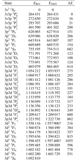
Table 2. Comparison of calculated and observed excitation energies in Ni XVII in cm−1.
State ERCI ENIST ∆E
3s2 1S 0 0 0 3s3p3P◦0 264 431 264 431 0 3s3p3P◦ 1 272 650 272 634 16 3s3p3P◦ 2 293 707 293 686 21 3s3p1P◦1 401 590 401 302 288 3p2 3P 0 628 065 627 914 151 3p2 1D 2 639 086 638 820 266 3p2 3P1 643 914 643 807 107 3p2 3P 2 669 689 669 535 154 3p2 1S0 755 195 754 513 682 3s3d3D1 771 391 771 268 123 3s3d3D 2 773 061 772 953 108 3s3d3D3 775 691 775 567 124 3s3d1D 2 865 079 864 465 614 3p3d3F◦ 2 1 054 212 1 053 937 275 3p3d3F◦3 1 068 917 1 068 632 285 3p3d1D◦ 2 1 081 412 1 081 126 286 3p3d3F◦ 4 1 086 391 1 086 107 284 3p3d3D◦1 1 115 712 1 115 521 191 3p3d3D◦ 2A 1 118 619 1 118 392 227 3p3d3D◦3 1 133 959 1 133 775 184 3p3d3P◦ 0 1 136 049 1 135 732 317 3p3d3P◦1 1 136 356 1 136 123 233 3p3d3D◦2B 1 136 892 1 136 643 249 3p3d1F◦ 3 1 209 617 1 209 017 600 3p3d1P◦1 1 223 592 1 222 730 862 3d2 3F 2 1 558 116 1 557 900? 216 3d2 3F 3 1 560 874 1 560 490 384 3d2 3F4 1 564 179 1 563 822 357 3d2 1D 2 1 595 636 1 594 821 815 3d2 3P 0 1 598 455 1 597 400? 1055 3d2 3P1 1 599 485 1 598 889 596 3d2 1G 4 1 602 182 1 601 404 778 3d2 3P2 1 602 280 1 601 729 551 3d2 1S 0 1 692 810
Notes. ERCIare energies that include low-frequency Breit, vacuum
po-larization, and self-energy corrections from present calculations. ENIST
observed energies from the NIST Atomic Spectra Database (ver. 5.3;
Kramida et al. 2015). Energies for all states in Ni XVII as well as en-ergies for the ions Ca IX – As XXII and Kr XXV are available at the CDS.
obtained with this approach are, however, not unique and this is further discussed in the next section.
3. Results and discussion 3.1. Energies
In Table1we present the computed excitation energies for the 35 lowest levels in Fe XV belonging to the 3l3l0configurations as functions of the increasing active sets of orbitals labeled with the highest principal quantum number n of the orbitals in the set. For comparison, observed energies from the NIST Atomic Spectra Database (ver. 5.3; Kramida et al. 2015) are given as well. The relative differences between theory and observation are 0.122%, 0.49%, 0.050% and 0.041% for calculations based on
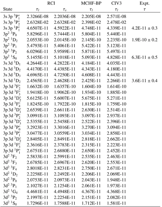
Table 3. Lifetimes in s. for Fe XV. τland τvare lifetimes in length and velocity form, respectively.
RCI MCHF-BP CIV3 Expt.
State τl τv τl τl τ
3s 3p3P◦1 2.3266E-08 2.2036E-08 2.205E-08 2.571E-08 3s 3p3P◦2 2.6328E-02 2.6328E-02 2.398E-02 2.478E-02
3s 3p1P◦1 4.6507E-11 4.5922E-11 4.748E-11 4.339E-11 4.2E-11 ± 0.3 3p2 3P
0 5.8296E-11 5.7444E-11 5.804E-11 5.440E-11
3p2 1D
2 2.0553E-10 2.0145E-10 2.145E-10 2.235E-10 1.9E-10 ± 0.2
3p2 3P
1 5.4793E-11 5.4061E-11 5.422E-11 5.123E-11
3p2 3P
2 6.0296E-11 5.9589E-11 5.871E-11 5.497E-11
3p2 1S
0 5.1455E-11 5.1018E-11 5.093E-11 4.828E-11 6.3E-11 ± 0.5
3s 3d3D
1 4.2644E-11 4.2822E-11 4.184E-11 4.035E-11
3s 3d3D2 4.4170E-11 4.4385E-11 4.343E-11 4.180E-11
3s 3d3D3 4.6965E-11 4.7250E-11 4.608E-11 4.443E-11
3s 3d1D2 2.4565E-11 2.4628E-11 2.425E-11 2.266E-11 3.6E-11 ± 0.4
3p 3d3F◦2 1.6632E-10 1.6357E-10 1.604E-10 1.614E-10 3p 3d3F◦
3 1.9418E-10 1.9062E-10 1.934E-10 1.885E-10
3p 3d1D◦
2 5.6125E-11 5.6007E-11 5.675E-11 5.271E-11
3p 3d3F◦
4 1.8245E-10 1.7922E-10 1.815E-10 1.759E-10
3p 3d3D◦
1 2.6539E-11 2.6611E-11 2.630E-11 2.514E-11
3p 3d3P◦
2 3.0991E-11 3.1093E-11 3.097E-11 2.937E-11
3p 3d3D◦
3 2.5355E-11 2.5458E-11 2.522E-11 2.396E-11
3p 3d3P◦0 3.2923E-11 3.3016E-11 3.270E-11 3.094E-11 3p 3d3P◦1 3.0477E-11 3.0559E-11 3.034E-11 2.858E-11 3p 3d3D◦2 2.8405E-11 2.8491E-11 2.818E-11 2.662E-11 3p 3d1F◦3 2.3616E-11 2.3783E-11 2.315E-11 2.223E-11 3p 3d1P◦1 2.6751E-11 2.6880E-11 2.650E-11 2.452E-11 3d2 3F
2 2.5833E-11 2.5991E-11 2.535E-11 2.463E-11
3d2 3F
3 2.6785E-11 2.6967E-11 2.620E-11 2.553E-11
3d2 3F
4 2.8018E-11 2.8231E-11 2.750E-11 2.671E-11
3d2 1D
2 2.2258E-11 2.2492E-11 2.206E-11 2.069E-11
3d2 3P
0 2.0753E-11 2.0973E-11 2.043E-11 1.948E-11
3d2 3P
1 2.1027E-11 2.1254E-11 2.061E-11 1.973E-11
3d2 1G4 4.4681E-11 4.4948E-11 4.367E-11 4.368E-11
3d2 3P2 2.1997E-11 2.2254E-11 2.151E-11 2.082E-11
3d2 1S0 1.7296E-11 1.7588E-11 1.712E-11 1.581E-11
Notes. RCI present calculations, MCHF-BP calculations byFroese Fischer et al.(2006), CIV3 calculations byAggarwal et al.(2007) and Expt. beam-foil measurements byHutton et al.(1988).
the expansion from the MR and the expansions from SD excita-tions to orbital sets with the highest principal quantum numbers n = 6, 7, 8. Looking more carefully at Table1it is seen that the triplet states show better convergence properties than the singlet states. For the singlet states the relative differences between the-ory and observation are 0.233%, 0.789%, 0.106% and 0.073% and the singlet states are not fully converged with respect to the orbital set. Adding a few orbital layers would improve the ex-citation energies, but would add to the total computation time. Differences in convergence rates are further analyzed and dis-cussed inJönsson et al.(2016). In Table2the computed excita-tion energies for Ni XVII (the full table for Ca IX – As XXII and Kr XXV is available at the CDS) based on the largest orbital set n = 8 are displayed together with observed energies from the NIST Atomic Spectra Database (ver. 5.3;Kramida et al. 2015). The differences between the computed and observed energies are
also given. For Kr XXV, excitation energies from accurate many-body perturbation calculations bySi et al.(2015) can be used for further comparisons.
The agreement between the computed excitation energies and the observed energies is generally very good, although the calculations give somewhat too high excitations energies for the states belonging to the 3l4l0and 3s5l configurations. For these
states typical differences are between 1000 cm−1and 2000 cm−1, which translates to relative differences of theory and observation between 0.05% and 0.1%. The difference between calculations and observations can be explained by the fact that the current cal-culations extend to many configurations and that the calcal-culations are not fully converged with respect to the orbital basis. The dif-ference is also due to the fact that core-core electron correlation were neglected, the effect of which is to lower the energies of the higher lying states. There are many states for which theory
and observations do not agree at all. An example is 3s4d1D2,
where the difference is −4488 cm−1 in Sc X and 6498 cm−1
in Ti XI. These disagreements may be due to difficulties in identification or labeling of levels derived from observed data. The present data are useful in validating the identification of levels.
As for most calculations involving states of many configura-tions there are labeling problems (Jönsson et al. 2013a). States are often labeled by the leading term of the wave function LS J-percentage composition. For closely lying interacting states with the same J, the leading term can be the same. To resolve this the label can be based on more terms of the composition. A sim-pler solution is to add an extra index to the leading term of the composition. We choose the latter solution. For example, the two J= 3 states in Fe XV at 2 316 401 cm−1and 2 333 084 cm−1both
have the leading term 3p4d3D3. These two states were labeled
3p4d3D
3 aand 3p4d3D3 b, respectively. It is important to
real-ize that the wave function LS J-percentage composition depends on the details of the calculation, and thus two calculations can have slight differences in compositions leading to differences in labels.
3.2. Lifetimes
Lifetimes of the excited states were calculated from E1 and M1 transition rates. The contributions to the lifetimes from E2 and higher multipoles are negligible. In Table 3 the present lifetimes for the 84 lowest states in Fe XV in length and ve-locity form are compared with lifetimes from the multiconfig-uration Hartree-Fock Breit-Pauli (MCHF-BP) calculations by Froese Fischer et al. (2006) and with the CIV3 calculations by Aggarwal et al. (2007). Included in the table are also lifetimes from beam-foil measurements byHutton et al.(1988).
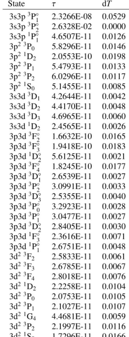
The average relative difference between the lifetimes in the length and velocity forms from the present calculation is less than 0.52%, which is highly satisfactory. This difference can be seen as an internal validation of the accuracy. The differences between the present lifetimes in the length form and the life-times byFroese Fischer et al.(2006) andAggarwal et al.(2007) are 1.37% and 4.45%, respectively. Comparing theoretical and experimental lifetimes we see that they do not agree very well. This may be due to large uncertainties in the beam-foil measure-ments as discussed inZou et al.(1999). In Table4the computed lifetimes in length form and the uncertainty estimators dT are displayed for Fe XV (the full table for Ca IX – As XXII and Kr XXV is available at the CDS) based on the largest orbital set n= 8.
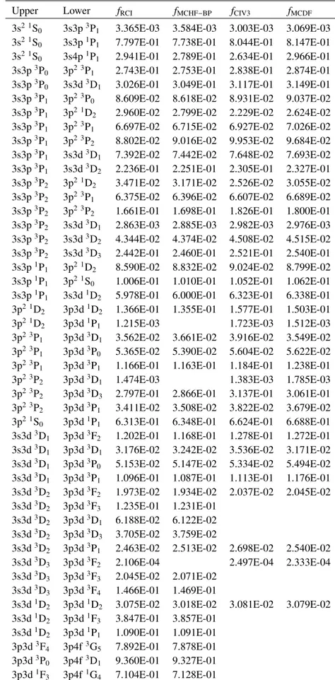
3.3. Oscillator strengths and transition rates
In Table 5 the present oscillator strengths in the length form for selected transitions in Fe XV are compared with values from the MCHF-BP calculations byFroese Fischer et al.(2006) and with values from the CIV3 and MCDHF calculations by Aggarwal et al. (2007). Values from the present calcula-tions and the MCHF-BP calculacalcula-tions agree to within 1.53%. The agreement with the CIV3 and MCDHF calculations by Aggarwal et al. (2007) is 8.42% and 6.50%, respectively. The results of the comparisons are explained by the fact that the RCI and MCHF-BP calculations include more electron correlation ef-fects than do the CIV3 and MCDHF calculations. Due to the neglected electron correlation two the latter calculations are be-lieved to be somewhat less accurate.
Table 4. Lifetimes in s for Fe XV.
State τ dT 3s3p3P◦1 2.3266E-08 0.0529 3s3p3P◦ 2 2.6328E-02 0.0000 3s3p1P◦1 4.6507E-11 0.0126 3p2 3P0 5.8296E-11 0.0146 3p2 1D 2 2.0553E-10 0.0198 3p2 3P1 5.4793E-11 0.0133 3p2 3P 2 6.0296E-11 0.0117 3p2 1S 0 5.1455E-11 0.0085 3s3d3D1 4.2644E-11 0.0042 3s3d3D 2 4.4170E-11 0.0048 3s3d3D 3 4.6965E-11 0.0060 3s3d1D2 2.4565E-11 0.0026 3p3d3F◦ 2 1.6632E-10 0.0165 3p3d3F◦ 3 1.9418E-10 0.0183 3p3d1D◦2 5.6125E-11 0.0021 3p3d3F◦ 4 1.8245E-10 0.0177 3p3d3D◦1 2.6539E-11 0.0027 3p3d3P◦ 2 3.0991E-11 0.0033 3p3d3D◦ 3 2.5355E-11 0.0040 3p3d3P◦0 3.2923E-11 0.0028 3p3d3P◦ 1 3.0477E-11 0.0027 3p3d3D◦2 2.8405E-11 0.0030 3p3d1F◦ 3 2.3616E-11 0.0071 3p3d1P◦ 1 2.6751E-11 0.0048 3d2 3F2 2.5833E-11 0.0061 3d2 3F 3 2.6785E-11 0.0067 3d2 3F4 2.8018E-11 0.0076 3d2 1D2 2.2258E-11 0.0104 3d2 3P 0 2.0753E-11 0.0105 3d2 3P1 2.1027E-11 0.0107 3d2 1G 4 4.4681E-11 0.0059 3d2 3P 2 2.1997E-11 0.0116 3d2 1S0 1.7296E-11 0.0166
Notes.τ is lifetime in length form and dT is the uncertainty estimator given by Eq. (2). Lifetimes for all states in Fe XV as well as lifetimes for the ions Ca IX – As XXII and Kr XXV are available at the CDS.
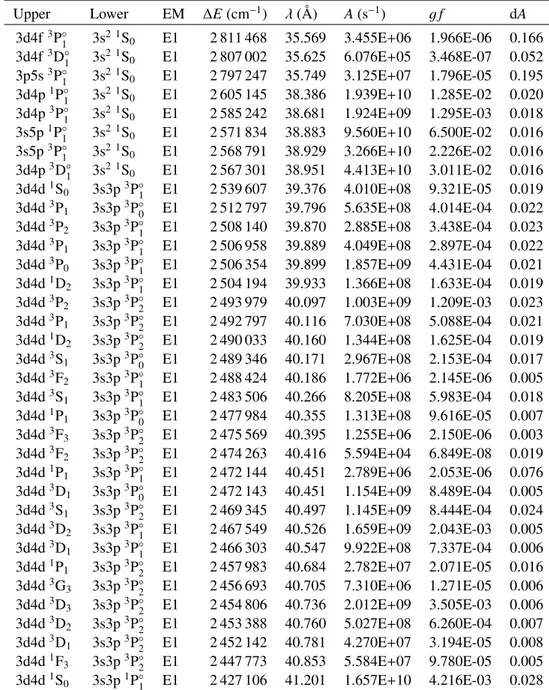
In Table 6 the transition energies, wavelengths, transition rates A, and weighted oscillator strengths g f are given for Fe XV (the full table for Ca IX – As XXII and Kr XXV is available at the CDS). All E1 and M1 transitions with rates A larger than 104 s−1 are displayed. Transition data are also given for
transi-tions with rates A greater than a fraction 10−4of the sum of the A-values for transitions from the upper level. For the E1 tran-sitions also the uncertainty indicator dA is given. For most of the stronger E1 transitions dA is below 1%. For the weaker tran-sitions the situation is somewhat different. While many of the weaker transitions have dA in the range from a few percent up to 10% there are also many transitions for which dA is considerably larger. These transitions are often so called two-electron one-photon transitions for which the configurations involved in the transitions differ by two electrons. For two-electron one-photon transitions the rate between two states is determined, not from the major CSFs that define the label, but from other CSFs of the wave function expansion, often CSFs that are part of the MR set. We take the 3s5d3D
2−3p4s3Po2transition in Ca IX at 499.614 Å
Table 5. Oscillator strengths f for selected transitions in Fe XV.
Upper Lower fRCI fMCHF−BP fCIV3 fMCDF
3s2 1S
0 3s3p3P1 3.365E-03 3.584E-03 3.003E-03 3.069E-03
3s2 1S
0 3s3p1P1 7.797E-01 7.738E-01 8.044E-01 8.147E-01
3s2 1S
0 3s4p1P1 2.941E-01 2.789E-01 2.634E-01 2.966E-01
3s3p3P
0 3p2 3P1 2.743E-01 2.753E-01 2.838E-01 2.874E-01
3s3p3P
0 3s3d3D1 3.026E-01 3.049E-01 3.117E-01 3.149E-01
3s3p3P
1 3p2 3P0 8.609E-02 8.618E-02 8.931E-02 9.037E-02
3s3p3P1 3p2 1D2 2.960E-02 2.799E-02 2.229E-02 2.624E-02
3s3p3P1 3p2 3P1 6.697E-02 6.715E-02 6.927E-02 7.026E-02
3s3p3P1 3p2 3P2 8.802E-02 9.016E-02 9.953E-02 9.684E-02
3s3p3P
1 3s3d3D1 7.392E-02 7.442E-02 7.648E-02 7.693E-02
3s3p3P
1 3s3d3D2 2.236E-01 2.251E-01 2.305E-01 2.327E-01
3s3p3P
2 3p2 1D2 3.471E-02 3.171E-02 2.526E-02 3.055E-02
3s3p3P
2 3p2 3P1 6.375E-02 6.396E-02 6.607E-02 6.689E-02
3s3p3P
2 3p2 3P2 1.661E-01 1.698E-01 1.826E-01 1.800E-01
3s3p3P
2 3s3d3D1 2.863E-03 2.885E-03 2.982E-03 2.976E-03
3s3p3P2 3s3d3D2 4.344E-02 4.374E-02 4.508E-02 4.515E-02
3s3p3P2 3s3d3D3 2.442E-01 2.460E-01 2.521E-01 2.540E-01
3s3p1P1 3p2 1D2 8.590E-02 8.832E-02 9.024E-02 8.799E-02
3s3p1P1 3p2 1S0 1.006E-01 1.010E-01 1.052E-01 1.062E-01
3s3p1P
1 3s3d1D2 5.978E-01 6.000E-01 6.323E-01 6.338E-01
3p2 1D
2 3p3d1D2 1.366E-01 1.355E-01 1.577E-01 1.503E-01
3p2 1D
2 3p3d1P1 1.215E-03 1.723E-03 1.512E-03
3p2 3P
1 3p3d3D1 3.562E-02 3.661E-02 3.916E-02 3.549E-02
3p2 3P
1 3p3d3P0 5.365E-02 5.390E-02 5.604E-02 5.622E-02
3p2 3P1 3p3d3P1 1.166E-01 1.163E-01 1.184E-01 1.238E-01
3p2 3P2 3p3d3D1 1.474E-03 1.383E-03 1.785E-03
3p2 3P2 3p3d3D3 2.797E-01 2.866E-01 3.137E-01 3.061E-01
3p2 3P2 3p3d3P1 3.411E-02 3.508E-02 3.822E-02 3.679E-02
3p2 1S
0 3p3d1P1 6.313E-01 6.348E-01 6.624E-01 6.688E-01
3s3d3D
1 3p3d3F2 1.202E-01 1.168E-01 1.278E-01 1.272E-01
3s3d3D
1 3p3d3D1 3.176E-02 3.242E-02 3.536E-02 3.171E-02
3s3d3D
1 3p3d3P0 5.153E-02 5.147E-02 5.334E-02 5.494E-02
3s3d3D
1 3p3d3P1 1.096E-01 1.087E-01 1.113E-01 1.176E-01
3s3d3D2 3p3d3F2 1.973E-02 1.934E-02 2.037E-02 2.045E-02
3s3d3D2 3p3d3F3 1.235E-01 1.231E-01
3s3d3D2 3p3d3D1 6.188E-02 6.122E-02
3s3d3D2 3p3d3D3 3.705E-02 3.759E-02
3s3d3D
2 3p3d3P1 2.463E-02 2.513E-02 2.698E-02 2.540E-02
3s3d3D
3 3p3d3F2 2.106E-04 2.497E-04 2.333E-04
3s3d3D
3 3p3d3F3 2.045E-02 2.071E-02
3s3d3D
3 3p3d3F4 1.466E-01 1.469E-01
3s3d1D
2 3p3d1D2 3.075E-02 3.018E-02 3.081E-02 3.079E-02
3s3d1D2 3p3d1F3 3.847E-01 3.857E-01 3s3d1D2 3p3d1P1 1.090E-01 1.091E-01 3p3d3F4 3p4f3G5 7.892E-01 7.878E-01 3p3d3P0 3p4f3D1 9.360E-01 9.327E-01 3p3d1F 3 3p4f1G4 7.104E-01 7.128E-01
Notes. fRCIpresent work in length form, fMCHF−BPcalculations byFroese Fischer et al.(2006), fCIV3and fMCDFare calculations byAggarwal et al.
Table 6. Transition data for Fe XV.
Upper Lower EM ∆E (cm−1) λ (Å) A(s−1) g f dA
3d4f3P◦ 1 3s 2 1S 0 E1 2 811 468 35.569 3.455E+06 1.966E-06 0.166 3d4f3D◦ 1 3s 2 1S 0 E1 2 807 002 35.625 6.076E+05 3.468E-07 0.052 3p5s3P◦ 1 3s 2 1S 0 E1 2 797 247 35.749 3.125E+07 1.796E-05 0.195 3d4p1P◦ 1 3s 2 1S 0 E1 2 605 145 38.386 1.939E+10 1.285E-02 0.020 3d4p3P◦1 3s2 1S0 E1 2 585 242 38.681 1.924E+09 1.295E-03 0.018 3s5p1P◦1 3s2 1S0 E1 2 571 834 38.883 9.560E+10 6.500E-02 0.016 3s5p3P◦1 3s2 1S0 E1 2 568 791 38.929 3.266E+10 2.226E-02 0.016 3d4p3D◦1 3s2 1S0 E1 2 567 301 38.951 4.413E+10 3.011E-02 0.016 3d4d1S0 3s3p3P◦1 E1 2 539 607 39.376 4.010E+08 9.321E-05 0.019 3d4d3P 1 3s3p3P◦0 E1 2 512 797 39.796 5.635E+08 4.014E-04 0.022 3d4d3P 2 3s3p3P◦1 E1 2 508 140 39.870 2.885E+08 3.438E-04 0.023 3d4d3P 1 3s3p3P◦1 E1 2 506 958 39.889 4.049E+08 2.897E-04 0.022 3d4d3P 0 3s3p3P◦1 E1 2 506 354 39.899 1.857E+09 4.431E-04 0.021 3d4d1D 2 3s3p3P◦1 E1 2 504 194 39.933 1.366E+08 1.633E-04 0.019 3d4d3P 2 3s3p3P◦2 E1 2 493 979 40.097 1.003E+09 1.209E-03 0.023 3d4d3P1 3s3p3P◦2 E1 2 492 797 40.116 7.030E+08 5.088E-04 0.021 3d4d1D2 3s3p3P◦2 E1 2 490 033 40.160 1.344E+08 1.625E-04 0.019 3d4d3S1 3s3p3P◦0 E1 2 489 346 40.171 2.967E+08 2.153E-04 0.017 3d4d3F2 3s3p3P◦1 E1 2 488 424 40.186 1.772E+06 2.145E-06 0.005 3d4d3S 1 3s3p3P◦1 E1 2 483 506 40.266 8.205E+08 5.983E-04 0.018 3d4d1P 1 3s3p3P◦0 E1 2 477 984 40.355 1.313E+08 9.616E-05 0.007 3d4d3F 3 3s3p3P◦2 E1 2 475 569 40.395 1.255E+06 2.150E-06 0.003 3d4d3F 2 3s3p3P◦2 E1 2 474 263 40.416 5.594E+04 6.849E-08 0.019 3d4d1P 1 3s3p3P◦1 E1 2 472 144 40.451 2.789E+06 2.053E-06 0.076 3d4d3D 1 3s3p3P◦0 E1 2 472 143 40.451 1.154E+09 8.489E-04 0.005 3d4d3S1 3s3p3P◦2 E1 2 469 345 40.497 1.145E+09 8.444E-04 0.024 3d4d3D2 3s3p3P◦1 E1 2 467 549 40.526 1.659E+09 2.043E-03 0.005 3d4d3D1 3s3p3P◦1 E1 2 466 303 40.547 9.922E+08 7.337E-04 0.006 3d4d1P1 3s3p3P◦2 E1 2 457 983 40.684 2.782E+07 2.071E-05 0.016 3d4d3G 3 3s3p3P◦2 E1 2 456 693 40.705 7.310E+06 1.271E-05 0.006 3d4d3D 3 3s3p3P◦2 E1 2 454 806 40.736 2.012E+09 3.505E-03 0.006 3d4d3D 2 3s3p3P◦2 E1 2 453 388 40.760 5.027E+08 6.260E-04 0.007 3d4d3D 1 3s3p3P◦2 E1 2 452 142 40.781 4.270E+07 3.194E-05 0.008 3d4d1F 3 3s3p3P◦2 E1 2 447 773 40.853 5.584E+07 9.780E-05 0.005 3d4d1S 0 3s3p1P◦1 E1 2 427 106 41.201 1.657E+10 4.216E-03 0.028
Notes. ∆E is transition energy in cm−1, λ is transition wavelength in Å, A is transition rate in s−1, g f is weighted oscillator strength, dA is
uncertainty estimator given by Eq. (2). Data for all transitions in Fe XV as well as for transitions in Ca IX – As XXII and Kr XXV are available at the CDS.
In LS J coupling the major contributors to the states are 0.75964323 3s5d3D2 −0.63064515 3p4f3D 2 0.06792502 3s5d1D 2 0.06676172 3p4f3F2 −0.06265593 3p4f1D 2 and 0.99191041 3p4s3P◦ 2 0.07887890 3s4p3P◦2 0.07366793 3d4p3P◦ 2 0.04500217 3p4d3P◦ 2.
Due to the selection rules of the transition operator, contributions to A are zero from the two dominating CSFs of the even state to
the dominating CSF of the odd state. The transition rate A is in-stead determined by contributions from different combinations of the remaining CSFs. The lack of contributions from the dominating CSFs together with many smaller and canceling contributions from the remaining CSFs often make the two-electron one-photon transitions weak and with large values of dA. Although important and challenging from a theoretical point of view, these weak transitions have little practical importance in modeling applications.
3.4. Summary and conclusions
MCDHF and subsequent RCI calculations were performed for states of the 3l3l0, 3l4l0and 3s5l configurations in the Mg-like ions Ca IX – As XXII and Kr XXV and excitation energies,
lifetimes, and transition data are presented for all ions. Excita-tion energies from the RCI calculaExcita-tions are in very good agree-ment with available observations for the lower states. For the higher states the calculated excitations energies are 1000 cm−1– 2000 cm−1 larger than energies from observations. There are
also anomalous differences, either positive or negative, between calculations and observations due to misindentifications. One example is the 3p4f configuration in Cu XVIII. Here the dif-ference between calculations and observations are 22 083 cm−1
and 1432 cm−1 for 3p4f 3D3 and 3p4f 3D2, respectively.
The former difference indicates a misidentification of observed data.
Lifetimes were internally validated by comparing values in length and velocity form. Lifetimes in the two forms differ in average at the 0.5% level. Systematic comparisons with the MCHF-BP calculations byFroese Fischer et al. (2006) showed that lifetimes from these two calculations differ on average only by 1.5%. Also for the oscillator strengths the present calcula-tions showed good consistency with the MCHF-BP with an aver-age relative difference of 1.5% for selected transitions in Fe XV. Uncertainties of the transition rates are estimated by dA, as sug-gested byEkman et al.(2014). For most of the stronger transi-tions, dA is below 1%. The transition rates for many of the weak two-electron one-photon transitions are highly uncertain, as in-dicated by large values of dA.
Acknowledgements. S.G. and P.J. acknowledge support from the Swedish Re-search Council under Grant 2015-04842.
References
Aggarwal, K. M., Tayal, V., Gupta, G. P., & Keenan, F. P. 2007,At. Data Nucl. Data Tables, 93, 615
Bhatia, A. K., & Landi, E. 2011,At. Data Nucl. Data Tables, 97, 189
Dyall, K. G., Grant, I. P., Johnson, C. T., Parpia, F. A., & Plummer, E. P. 1989, Comput. Phys. Commun., 55, 425
Ekman, J., Godefroid, M. R., & Hartman, H. 2014,Atoms, 2, 215
Hu, F., Mei, M., Han, C., et al. 2014,J. Quant. Spectrosc. Radiat. Trans., 149, 158
Fernandez-Menchero, L., Del Zanna, G., & Badnell, N. R. 2014,A&A, 572, A115
Froese Fischer, C. 2009,Phys. Scr. T, 134, 014019
Froese Fischer, C., Tachiev, G., & Irimia, A. 2006,At. Data Nucl. Data Tables, 92, 607
Froese Fischer, C., Godefroid, M., Brage, T., Jönsson, P., & Gaigalas, G. 2016, J. Phys. B: At. Mol. Opt. Phys., submitted
Gaigalas, G., Žalandauskas, T., & Rudzikas, Z. 2003,At. Data Nucl. Data Tables, 84, 99
Grant, I. P. 1974,J. Phys. B, 7, 1458
Grant, I. P. 2007, Relativistic Quantum Theory of Atoms and Molecules (New York: Springer)
Hutton, R., Engström, L., & Träbert, E. 1988,Nucl. Instrum. Meth. Phys. Res. B, 31, 294
Jönsson, P., & Froese Fischer, C. 1998,Phys. Rev. A, 57, 4967 Jönsson, P., Ekman, J., Gustafsson, S., et al. 2013a,A&A, 559, A100
Jönsson, P., Gaigalas, G., Biero´n, J., Froese Fischer, C., & Grant, I. P. 2013b, Comput. Phys. Commun., 184, 2197
Jönsson, P., Radži¯ut˙e, L., Gaigalas, G., et al. 2016,A&A, 585, A26
Kramida, A., Ralchenko, Yu., Reader, J., & NIST ASD Team 2015, NIST Atomic Spectra Database (ver. 5.3), available: http://physics.nist. gov/asd[2016, April 5] (Gaithersburg, MD: National Institute of Standards and Technology)
Landi, E. 2011,At. Data Nucl. Data Tables, 97, 587
Landi, E., & Bhatia A. K. 2014,At. Data Nucl. Data Tables, 100, 1519 Massacrier, G., & Artru, M.-C. 2012,A&A, 538, A52
McKenzie, B. J., Grant, I. P., & Norrington, P. H. 1980,Comput. Phys. Commun., 21, 233
Olsen, J., Godefroid, M., Jönsson, P., Malmqvist, P. Å., & Froese Fischer, C. 1995,Phys. Rev. E, 52, 4499
Safronova, U. I., Johnson, W. R., & Berry, H. G. 2000,Phys. Rev. A, 61, 052503
Santana, J. A., & Träbert, E. 2015,Phys. Rev. A, 91, 022503
Si, R., Guo, X. L., Yan, J., et al. 2015,J. Phys. B: At. Mol. Opt. Phys., 48, 175004 Zou, Y., Hutton, R., Huldt, S., et al. 1999,Phys. Scr.. T, 80, 460