IN
DEGREE PROJECT COMPUTER SCIENCE AND ENGINEERING, SECOND CYCLE, 30 CREDITS
,
STOCKHOLM SWEDEN 2017
Fast and Scalable Static Analysis
using Deterministic Concurrency
PATRIK ACKLAND
KTH ROYAL INSTITUTE OF TECHNOLOGY
Fast and Scalable Static Analysis using
Deterministic Concurrency
PATRIK ACKLAND
Master in Computer Science Date: July 10, 2017
Supervisor: Philipp Haller Examiner: Mads Dam
Swedish title: Snabb och skalbar statisk analys med hjälp av deterministisk samtida exekvering
i
Abstract
This thesis presents an algorithm for solving a subset of static analysis data flow prob-lems known as Interprocedural Finite Distribute Subset probprob-lems. The algorithm, called IFDS-RA, is an implementation of the IFDS algorithm which is an algorithm for solving such problems. IFDS-RA is implemented using Reactive Async which is a deterministic, concurrent, programming model. The scalability of IFDS-RA is compared to the state-of-the-art Heros implementation of the IFDS algorithm and evaluated using three different taint analyses on one to eight processing cores. The results show that IFDS-RA performs better than Heros when using multiple cores. Additionally, the results show that Heros does not take advantage of multiple cores even if there are multiple cores available on the system.
ii
Sammanfattning
Detta examensarbete presenterar en algoritm för att lösa en klass av problem i statisk analys känd som Interprocedural Finite Distribute Subset problem. Algoritmen, IFDS-RA, är en implementation av IFDS algoritmen som är utvecklad för att lösa denna typ av problem. IFDS-RA använder sig av Reactive Async som är en deterministisk programme-ringsmodell för samtida exekvering av program. Prestendan evalueras genom att mäta exekveringstid för tre stycken taint analyser med en till åtta processorkärnor och jämförs med state-of-the-art implementationen Heros. Resultaten visar att IFDS-RA presterar bätt-re än Heros när de använder sig av flera processorkärnor samt att Heros inte använder sig av flera processorkärnor även om de finns tillgängliga.
iii
Acknowledgments
I would like to thank my supervisor Philipp Haller for providing feedback and thought-ful insights. I would also like to thank Michael Eichberg for his comments and feedback during this process as well as for letting me run the experimental evaluation on his ma-chine. Finally, I would like to say thank you to Erik and Olof who were part of my thesis group at KTH for their peer reviews during the semester.
Contents
Contents iv 1 Introduction 1 1.1 Motivation . . . 1 1.2 Problem Statement . . . 2 1.3 Contribution . . . 2 1.4 Limitations . . . 21.5 Ethics and Sustainability . . . 3
1.6 Outline . . . 3 2 Background 4 2.1 Scala Syntax . . . 4 2.2 Static Analysis . . . 4 2.2.1 Taint Analysis . . . 5 2.2.2 FlowTwist . . . 6
2.3 Interprocedural Finite Distributive Subset . . . 6
2.3.1 The IFDS Algorithm . . . 7
2.3.2 Extensions to the IFDS Algorithm . . . 9
2.3.3 The Heros Implementation . . . 13
2.4 Reactive Async . . . 15
2.4.1 Cell Completer Operators . . . 15
2.4.2 Callbacks . . . 15
2.4.3 Dependencies . . . 16
2.4.4 Handler Pool . . . 16
2.4.5 Example . . . 16
3 Reactive Async Based IFDS 18 3.1 The Approach . . . 18
3.2 Implementation . . . 19
3.3 Comparison with Heros . . . 20
4 Experimental Setup 23 4.1 Metrics . . . 23 4.2 Test Setup . . . 23 4.3 Taint Analysis . . . 24 4.3.1 Test Setup 1 . . . 25 4.3.2 Test Setup 2 . . . 25 iv
CONTENTS v 4.3.3 Test Setup 3 . . . 25 5 Results 26 5.1 Test Setup 1 . . . 26 5.2 Test Setup 2 . . . 28 5.3 Test Setup 3 . . . 29 6 Related Work 30 6.1 Concurrent IFDS . . . 30
6.2 Extensions to the IFDS Algorithm . . . 30
6.2.1 IFDS With Correlated Method Calls . . . 31
6.2.2 Boomerang . . . 31
6.2.3 T.J. Watson Libraries for Analysis . . . 31
7 Discussion 32 7.1 Discussion . . . 32
7.2 Future Work . . . 34
7.3 Conclusion . . . 34
Bibliography 35
Chapter 1
Introduction
1.1
Motivation
In recent years we have come to see that processor cores are no longer getting faster and faster. To keep up with Moore’s law, computers now utilize multiple processing cores to improve performance by executing tasks in parallel. However, writing code that takes advantage of multiple cores is not an easy task [1]. Many programmers are not trained to write programs for multi-core systems which leads to problems with the program code not acting correctly because of data races and more. Writing programs for multi-core sys-tems can also lead to programs that are implemented correctly but that do not perform faster on multiple cores. This is due to the fact that even though the program is written to use multiple cores, it is written in a way which does not utilize them efficiently. One solution to this is to use a programming model which abstracts away from the details of concurrent programming such as threads, and locks. Examples of such models are Fu-tures [2] and Promises [3] or Reactive Async [4].
One area that benefits from faster programs is static analysis. Static analysis is an im-portant tool for programmers to use to reason about their programs. Static analysis can tell developers things about their program that can be difficult to see by just looking at the code. Examples of different use cases for static analysis are within computer secu-rity, to tell how sensitive parts of an application might be affected by certain inputs, or variable type analysis to compute a set of possible types for each variable in a program. The analyses can be used to improve programmer productivity by helping programmers solve bugs in their code that might be hard to discover otherwise and also increase con-fidence in the code being written. In order for static analysis to be useful it needs to be fast. A tool that takes too long would not be practical since it has the opposite effect and instead slows down the programmer.
The Interprocedural Finite Distributive Subset (IFDS) is a subset of static analysis problems that all have certain properties. Examples of static analyses that are IFDS prob-lems are taint analysis, type analysis, and truly-live-variable analysis. All IFDS probprob-lems can be solved with the IFDS algorithm originally developed by Reps et al. [5]. Since the IFDS algorithm can be used to solve a number of static analysis problems, performance improvements for the IFDS algorithm would mean performance improvements for a wide range of static analysis problems.
2 CHAPTER 1. INTRODUCTION
1.2
Problem Statement
This thesis presents an implementation of the IFDS algorithm [5] called IFDS-RA based on Reactive Async [4] and investigates how it compares to the state of the art implemen-tation Heros [6]. The problem statement in this thesis can be summarized with the fol-lowing research questions:
• How does the forwards IFDS algorithm based on Reactive Async perform com-pared to the state-of-the-art Heros implementation in terms of scalability.
• How does the bidirectional IFDS algorithm based on Reactive Async perform com-pared to the state-of-the-art Heros implementation in terms of scalability.
This will be investigated through a taint analysis [7] formulated as an IFDS problem which is then solved with the previously mentioned IFDS algorithms. The taint analysis will use SOOT [8] to generate an interprocedural control flow graph of the code being analyzed. The analyses will be run multiple times using 1,2, . . . , 8 cores to determine the performance and scalability of the algorithms.
1.3
Contribution
The contributions of this thesis are:
• A novel, deterministic concurrent implementation of IFDS in Scala based on Reac-tive Async;
• A novel, deterministic concurrent implementation of bidirectional IFDS in Scala based on Reactive Async;
• New experimental results for the practical evaluation of Reactive Async; • New experimental results for the practical evaluation of Heros.
IFDS-RA is available as an open source project on GitHub1.
1.4
Limitations
This thesis is only concerned with the scalability of the two algorithms in terms of how they perform on 1, 2, . . . , 8 cores. Memory usage of the two algorithms is not analyzed or discussed but could be of interest in future work. Additionally another limitation is that the machine the evaluation is run on belongs to someone else which means there is no control over what other tasks might be run at the same time as the evaluation. Care was taken to make sure the machine was idle before running the algorithms.
CHAPTER 1. INTRODUCTION 3
1.5
Ethics and Sustainability
Fast and scalable algorithms that can be used for static analysis is useful in the sense that it can help programmers ensure that their code is written correctly. It can add confidence in programs written to make sure there are no security leaks in the program. This is im-portant for many companies and society as a whole. Because a lot of sensitive informa-tion is becoming digital, keeping this informainforma-tion secure is an important task. For a large system it is necessary to have a fast algorithm that can analyze the large code base in a reasonable amount of time.
Additionally, when dealing with computers and processing power, environmental sustainability cannot be ignored. Carbon emissions from data centers are large enough to equal carbon emissions of certain countries and is expected to increase more in the fu-ture [9]. Basmadjian and de Meer [10] has shown that the power consumption of multi-core systems is lower than the sum of each individual multi-core, because some components consume a constant amount of power regardless of the number of cores. This means faster algorithms on multi-core systems could have environmental benefits. However the power consumption of IFDS-RA is not analyzed in this work.
From an ethical standpoint, while no tests were performed on humans or animals, there are a number of ethical considerations from the point of view of conducting re-search. Efforts have been made to describe every step of the implementation presented in this thesis and how the experimental setup was executed to make sure the results can be reproduced. Additionally, test cases for the algorithm has been written to ensure cor-rectness of the results. Finally, because this thesis presents an algorithm for solving static analyses problems and particularly a taint analysis, which can be used to find to find flaws in programs, the ethical aspects of making this work public, especially the code, should be considered. However, because this thesis only presents an algorithm that can run a taint analysis, and uses a publicly available taint analysis, FlowTwist, for the evalu-ation, and compares the results to Heros, which is also publicly available, this work does not introduce any new tools that were not already available.
1.6
Outline
The outline of the report is as follows. Chapter 2 discusses the background necessary for understanding the thesis. This includes the theory behind IFDS problems, the IFDS al-gorithm, extensions to the IFDS alal-gorithm, the Heros implementation, static taint anal-ysis, and the Reactive Async library. Chapter 3 explains the approach and implementa-tion of the IFDS-RA algorithm. Chapter 4 discusses the experimental setup used for the taint analysis and how it is executed. Chapter 5 shows the results of the taint analyses for Heros and IFDS-RA Chapter 6 discusses related work that has been done on the IFDS algorithm and finally Chapter 7 discusses the results of the taint analysis for both the forwards algorithm and the bidirectional algorithm, mentions possible future work and ends with conclusions.
Chapter 2
Background
2.1
Scala Syntax
This section briefly explains part of the Scala language that appear in this thesis for those that have no background in Scala. Scala is a statically typed language which runs on top of the Java Virtual Machine. The Scala code in this thesis is similar to Java and is used in an object-oriented way. Table 2.1 shows the Scala keywords that are used in code exam-ples later and what they mean. In Scala, types come after names in variable declarations and method declarations. Finally, if the return keyword is omitted, the return value is the last expression in the method.
2.2
Static Analysis
Program code analysis can be either static or dynamic. Static analysis analyses program code without running it whereas dynamic analysis is reasoning about program code by executing it. Static analysis abstracts away from the execution of a program which has many variables such as user inputs, files, and more and reasons about conditions that hold for every execution of the program regardless of these variables. This leads to an analysis which holds for any execution of the program, although the results of the analy-sis might not be as exact as for a dynamic analyanaly-sis [11]. A dynamic analyanaly-sis on the other hand is performed at runtime and can give more detailed results compared to static anal-ysis. However, because a dynamic analysis depends on its input, it is difficult to draw
Table 2.1: Table of Scala keywords
Keyword Explanation def defines a method. val defines a final variable. var defines a non-final variable. trait similar to interface in Java.
case class immutable class which exposes its constructor parameters. Unit similar to void in Java.
Class[T] [and ] is used for generics. Same as Class<T> in Java.
CHAPTER 2. BACKGROUND 5
conclusions that hold for the program in general as well as finding input that covers the entire program code [11].
2.2.1 Taint Analysis
Taint analysis as described in this thesis is a static analysis which is concerned about data flow between sources and sinks which are defined by the user and are points of interest in the program code being analyzed [7]. The analysis taints data from sources and propagates the tainted data through the program code. If some tainted data reaches a sink, there is a path from a source to a sink. Taint analysis can be used for computer security to make sure sensitive data is not leaked to users. Taint analysis can be used both for confidentiality problems and integrity problems. For a confidentiality problem, sources are some sensitive part of the application and sinks are parts of the program code exposed to the user. For an integrity problem sources are public methods the user has access to and sinks are some sensitive part of the application code.
Consider the code blow which is a small Scala program, reproduced from a Java ex-ample in [6], which is used to represent how a taint analysis can be used to find leaks in the program code. We define secret() to be our source and println as our sink. The variable x is assigned some secret value which we do not want to expose to our user. In this example, secret() is considered our source of the tainted value. After the assign-ment to x, the analysis marks x as tainted. We provide x as an arguassign-ment to the func-tion bar which results in the parameter z in bar to be tainted. The variable z is then returned and assigned to y which means y is now tainted. Finally y is passed as an ar-gument to println which is our sink. We can see that a tainted value originating from our source has reached the sink.
def foo: Unit = {
var x: Int = secret()
var y: Int = 0 y = bar(x) println(y) }
def bar(z: Int): Int = { z
}
As mentioned, a taint analysis can be used for both integrity and confidentiality prob-lems. For an integrity problem, where sources are public methods and sinks are some sensitive part of the program code, a taint analysis as presented above would scale poorly. This is because the number of public methods outnumber the number of sinks so the al-gorithm would follow unnecessarily many paths, where most of them would not reach a sink [7]. Consider, as an example the Java Class Library. Every public method would be a source. Not all API methods use some sensitive part of the program code. Similarly a confidentiality problem where one is interested in whether or not sensitive data can leak from the application to a user, would face the same issue where not all access to the sensitive data would leak it through the public API. The solution to this is to run the al-gorithm in reverse. For an integrity problem, the alal-gorithm would start at the sinks, of
6 CHAPTER 2. BACKGROUND
which there are fewer, and propagate tainted values until they reach a source. One type of attack that a taint analysis can discover is a so called Confused Deputy Attack [12]. A confused deputy attack is when some part of the program code is tricked into perform-ing some operation which the user who invoked the operation does not have permission to do. Because it is a combination of a confidentiality issue and an integrity issue, a taint analysis would have to be run twice, once forwards and once backwards [7].
2.2.2 FlowTwist
FlowTwist is a state-of-the-art taint analysis developed by Lerch et al. [7] which is used for the evaluation described in Section 4. FlowTwist handles normal execution of Java programs such as assignments, calls, and returns. In FlowTwist, if an array index is tainted the entire array is considered to be tainted. This reflects the limitations of a taint anal-ysis since array indices might be user inputs which are unknown to a static analanal-ysis. FlowTwist is able to handle often used Java objects such as StringBuilders which are used by both developers and compilers. The flow functions used in FlowTwist is decided by a configuration class which provides configurations for the taint analyses used in the evaluation. Flow functions can easily be added or removed to the configuration to fit the need of the taint analyses being executed.
The FlowTwist taint analyses are examples of real security threats for the Java
lan-guage. It consists of two different types of taint analyses. One uses calls to Class.forName as sinks and the other uses calls to methods with annotation @CallerSensitive which has both parameters and has a return value as sinks.
FlowTwist is implemented using SOOT which is a static analysis library developed by Vallée-Rai et al. [8]. SOOT is used to construct a call-graph of the program code being analyzed. The algorithm used for call-graph construction is the default in SOOT which is an implementation of Class Hierarchy Analysis [13]. The call-graph represents the in-terprocedural flow of a program which means calling relations between methods. SOOT is also used to construct an interprocedural control flow graph which in addition to calls also has the flow inside a method. SOOT provides a three-address code intermediate rep-resentation of the program code being analyzed called Jimple which is more suitable for flow analysis as it consists of fewer operations than Java bytecode representation and is simpler to analyze [14]. Three-address code has the form x = y op z and is stack-less. FlowTwist is implemented using Jimple. Additionally, SOOT provides both a forwards call-graph and a backwards call-graph. The backwards graph is used when running the taint analysis in reverse.
2.3
Interprocedural Finite Distributive Subset
Interprocedural Finite Distributive Subset (IFDS) problems [5] is a set of data-flow prob-lems with the following properties:
• The set D of data-flow facts is finite.
• The domain of the flow functions is the power-set of D.
• The flow functions are distributive. This means that for a flow function f we have ∀d1, d2 ∈ 2D, f (d1 ∪ d2) = f (d1) ∪ f (d2).
CHAPTER 2. BACKGROUND 7
(a) Identity function (b) Gen/kill function
Figure 2.1: Data-flow graph
A flow function calculates the result of a statement on a set of facts. Facts are infor-mation that holds for the given statement and varies depending on the type of problem. Consider Figure 2.1, reproduced from [5]. The figure shows two examples of a flow func-tion being applied to a set of facts. In Figure 2.1a the identity funcfunc-tion f (S) = S is ap-plied to the upper set of facts which leaves all sets unchanged. Figure 2.1b is an example of generating facts (fact a) and killing facts (fact b) and leaving the rest of the facts un-changed (fact c). This is represented by the following function: f (S) = (S \ b) ∪ a. The fact 0 represents an empty fact and it always holds. Two 0-nodes will always be connected. It is used to generate facts unconditionally. Many different types of static analysis problems can be formulated as an IFDS problem such as taint analysis, type analysis, and more.
An IFDS problem operates on an exploded super graph. An exploded super graph is a graph where for each statement in a program, a node is created for each statement paired with every data-flow fact from d ∈ D ∪ {0}. This results in |D| + 1 nodes per statement and (|D|+1)×|Statements| in total. As an example, consider Figure 2.1a again, it has two statements and three data-flow facts (a, b, and c) which results in a total of (3 + 1) × 2 = 8 nodes.
2.3.1 The IFDS Algorithm
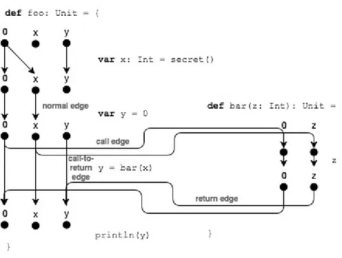
The original algorithm for solving IFDS problems was presented by Reps et al. [5]. The algorithm takes an exploded super graph of the program being analyzed as input and calculates for each node in the super graph what facts hold for that node. Figure 2.2 shows the exploded super graph for the code example used previously for the taint anal-ysis. The figure shows that a data flow problem when translated to an exploded super graph translates to a graph reachability problem where if, from a start point (s, 0), the node (n, d1) is reachable, there is a flow from the starting point of the program to
state-ment n where d1 holds.
The exploded super graph has different types of nodes and edges. The different kinds of nodes in the exploded super graph are:
• Call-site node: A node which represents a method call. • Exit-site node: A node which represents the exit of a method.
• Return-site node: A node to which the data flow returns after a method call. • Normal node: A node that is not a call-site, exit-site, or return-site node.
8 CHAPTER 2. BACKGROUND
Figure 2.2: Exploded super graph
There are also different kinds of edges that represent relations between nodes. The different kinds of edges in the graph are:
• Call edge: An edge which connect call-site nodes to the start point of the called procedure.
• Call-to-return edge: An edge which connects a call-site to the return-site of the call. Call-to-return edges are used to propagate facts that are not affected by the called procedure.
• Return edge: An edge which connects an exit-site node to the matching return-site for the call-site which called the procedure.
• Normal edge: An edge that is not a call, call-to-return, or return edge.
In Figure 2.2 the different types of edges are labeled. The call edge from x to z prop-agates facts from the call site to the start point of the method. The edge from y to y is a call-to-return edge which propagates facts not affected by the call to the return site matching the call site. The return edge z to y propagates facts to the return site of the call.
The pseudo code for the IFDS algorithm with the extensions described in Section 2.3.2 can be seen in Algorithm 1 with the methods for processing the different kinds of nodes explained in Algorithm 2. The algorithm works by keeping a global work list which initially has only the starting points for the algorithm. The work list is processed un-til it is empty and the algorithm then terminates. Every node is either handled as a call node, an exit node, or a normal node. The edges being propagated by the algorithm are represented as triples (d1, n, d2) where d1 is the fact which holds at the start of the
cur-rent method and (n, d2)is the exploded super graph node being propagated. The
CHAPTER 2. BACKGROUND 9
this it needs to support multiple start points and multiple return sites. This is because when running an algorithm in reverse, call sites become return sites and exit nodes be-come start points. While the forwards IFDS algorithm only has one starting point, it can have multiple exit sites which translates to multiple starting points for an IFDS algorithm run in reverse. The original IFDS algorithm did not support this but it is required for the bidirectional IFDS algorithm presented in Section 2.3.2.
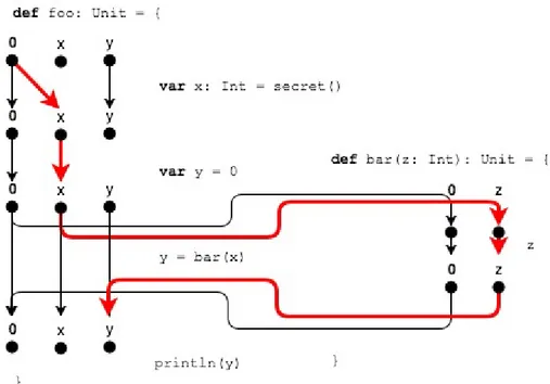
Figure 2.3 demonstrates how a taint analysis can be modeled as an IFDS problem. Like before, secret() is considered the source and println the sink. In the exploded super graph this is a graph reachability problem where we are wondering if data can flow from the return value of secret() into the println statement. This flow is marked in red in the figure. The data fact is propagated through the bar method and then re-turned and passed into the println statement. For a taint analysis problem, facts are among other things, what variables are tainted, while flow functions are used to propagate tainted values through the graph. Consider the statement var x: Int = secret(). This equals applying a flow function f ({}) = {x}. Before, there were no tainted values, and after applying the flow function, x is now tainted. In the graph this is represented by the edge from 0 to x.
Figure 2.3: Information flow in exploded super graph
2.3.2 Extensions to the IFDS Algorithm
This section provides a number of extensions that have been made to the original IFDS algorithm by Reps et al. [5]. First by Naeem et al. [15] who developed what is commonly referred to as the extended IFDS algorithm and then Lerch et al. [7] who developed the bidirectional IFDS algorithm.
10 CHAPTER 2. BACKGROUND
The Extended IFDS Algorithm
Naeem et al. [15] has further developed the original IFDS algorithm by Reps et al. [5] with a number of extensions. One of which is to compute the nodes of the super graph on demand. This makes the algorithm more memory efficient since there is no need to compute parts of the graph that are not needed for the analysis. This enables the algo-rithm to be useful for problems where the set of data-flow facts D in theory is very large but where only a subset is used during the analysis. Remember that the exploded super graph has approximately (|D| + 1) × |Statement| nodes. This is done by using flow func-tions that determine what facts hold for the node that is being propagated. The extended algorithm uses four different flow functions to compute facts. In the pseudo code in Al-gorithm 2 those are:
• CallFlow(callSite, calledMethod). Calculate which facts hold at the start of calledMethod for call at callSite.
• ReturnFlow(callSite, methodOfCallSite, exitSite, returnSite). Calculate which facts hold for returnSite in methodOfCallSite for the call originating from
callSitereturning from exitSite.
• CallToReturnFlow(callSite, returnSite) Calculate which facts hold for returnSite for call at callSite.
• NormalFlow(n, successor) Calculate which facts hold for successor. Another extension is to introduce two global data structures Incoming and
EndSummary. The latter is used to avoid having to process a method twice for the same incoming fact. If a fact a holds at the start of a method and, after propagating that fact through the method, b holds at the exit-site, there is no need to process the method again for a, since it will result in fact b at the exit site. Instead, after processing the method the first time, the exit site and facts that hold for it are stored in EndSummary for that particular starting point and fact. Next time, instead of propagating the fact through the method again, it can be retrieved from EndSummary. Similarly Incoming is used for efficiently propagating return flow from methods by storing the call site node and fact. When processing an exit node, the values in Incoming are used to get the call site and the fact which holds for that method. If the call-site node (c, d1) has been processed
preivously and c is a call-site for the method being processed currently, (c, d1)is stored
in Incoming for the start point of the current method and the fact which holds for that start point. This allows the algorithm to easily calculate the return flow to the return-site of c by querying Incoming and get the return return-sites of c. These can be seen in the pseudo code for the IFDS algorithm, in Algorithm 2, in lines 7–10 and 19–24 for EndSummaryand Incoming respectively.
Bidirectional IFDS Algorithm
Lerch et al. [7] has developed a bidirectional version of the IFDS algorithm which is based on the extended IFDS algorithm by Naeem et al. [15]. It starts at the inner layer of the application code and runs one solver in a forwards direction and one solver in a back-wards direction. Internally it has two solvers which knows about each other. The
CHAPTER 2. BACKGROUND 11
Algorithm 1IFDS algorithm with extensions by [15, 7]
1: P athEdge ← ∅
2: W orkList ← ∅
3: Incoming ← EmptyM ap
4: EndSummary ← EmptyM ap
5: functionTABULATE(startingPoints)
6: for all s ∈ startingP oints do 7: P athEdge ← {(0, s, 0)} 8: W orkList ← {(0, s, 0)} 9: FORWARDTABULATESLRPS 10: 11: functionPROPAGATE(d1, n, d2) 12: if (d1, n, d2) /∈ P athEdge then 13: WORKLIST.ADD((d1, n, d2)) 14:
15: functionPROPAGATEUNBALANCED(n, d2)
16: PROPAGATE(0, n, d2)
17:
18: functionFORWARDTABULATESLRPS 19: while W orkList 6= ∅ do
20: (d1, n, d2) ←WORKLIST.GET
21: if n ∈ CallN odes then 22: PROCESSCALL(d1, n, d2)
23: else if n ∈ ExitN odes then 24: PROCESSEXIT(d1, n, d2)
25: else
12 CHAPTER 2. BACKGROUND
Algorithm 2Node-processing functions
1: functionPROCESSCALL(d1, n, d2)
2: for all calledM ethod ∈CALLEESOFCALLAT(n)do
3: for all startP oint ∈STARTPOINTSOF(calledM ethod)do 4: for all d3∈ CALLFLOW(n, calledM ethod)do
5: PROPAGATE(d3, startP oint, d3)
6: INCOMING(startP oint, d3).ADD((n, d2))
7: for all (ep, d4) ∈ENDSUMMARY((startP oint, d3))do
8: for all retSite ∈RETURNSITESOFCALLAT(n)do
9: for all d5 ∈RETURNFLOW(n, calledM ethod, ep, retSite)do 10: PROPAGATE(d1, retSite, d5)
11: for all retSite ∈RETURNSITESOFCALLAT(n)do 12: for all d3 ∈ CALLTORETURNFLOW(n, retSite)do
13: PROPAGATE(d1, retSite, d5)
14:
15: functionPROCESSEXIT(d1, n, d2)
16: method ← METHODOF(n)
17: for all startP oint ∈STARTPOINTSOF(method)do 18: ENDSUMMARY(startP oint, d1).ADD((n, d2))
19: for all (c, d4) ∈INCOMING(startP oint, d1)do
20: for all retSite ∈RETURNSITESOFCALLAT(n)do 21: for all d5 ∈ RETURNFLOW(c, method, n, retSite)do
22: for all (d01, n0, d02) ∈ P athEdgedo 23: if n0 = c ∧ d02 = d4then
24: PROPAGATE(d01, retSite, d5)
25: if d1 =0 ∧INCOMING.EMPTYthen
26: for all c ∈CALLERSOF(method)do
27: for all retSite ∈RETURNSITESOFCALLAT(n)do 28: for all d5 ∈ RETURNFLOW(c, method, n, retSite)do
29: PROPAGATEUNBALANCED(retSite, d5)
30:
31: functionPROCESSNORMAL(d1, n, d2)
32: for all m ∈SUCCESSOROF(n)do
33: for all d3 ∈ NORMALFLOW(n, m)do
CHAPTER 2. BACKGROUND 13
Tabulatemethod of the bidirectional IFDS algorithm can be seen in Algorithm 4. It cre-ates one solver in each direction and provides them with references to each other. The bidirectional solver pauses propagations for unbalanced return flows of one solver until the other solver reaches the same node in the graph. That way, the solver is only con-cerned with edges that go from sources to sinks which reduces the amount of edges be-ing propagated. This requires another extension to the IFDS algorithm which makes it possible to handle unbalanced returns. An unbalanced return occurs when processing a return node for which there has not been an incoming call. For a traditional forwards IFDS problem this would not occur, but because the algorithm by Lerch et al. [7] starts at the inner layer of the program code it will eventually processes a return node for which there was no call-site already propagated.
In the pseudo code in Algorithm 3 this addition to the IFDS algorithm can be seen. An unbalanced return would only occur when 0 is the fact that holds for the method and incoming is empty for the start points of that method. An unbalanced return is propa-gated by setting the empty fact as the method fact. This extension is added at the end of the processExit method.
Algorithm 5 shows the extension to the IFDS algorithm for the bidirectional IFDS al-gorithm. The facts are augmented with a source object which is represented by the tuple (source, d2) which was previously just d2. When the algorithm does an unbalanced
re-turn, it checks if the other solver (forwards for the backwards analysis or backwards for the forwards analysis) has leaked the source for that path edge, and if it has it unpauses it for the other solver and propagates it, otherwise it adds it to the paused edges.
Algorithm 3Extension for unbalanced returns
25: if d1 =0 ∧INCOMING.EMPTYthen
26: for all c ∈CALLERSOF(method)do
27: for all retSite ∈RETURNSITESOFCALLAT(n)do 28: for all d5 ∈ RETURNFLOW(c, method, n, retSite)do
29: PROPAGATEUNBALANCED(retSite, d5)
Algorithm 4Bidirectional IFDS
1: functionTABULATE(startingPoints)
2: fwSolver ← IFDSSOLVER(startingPoints) 3: bwSolver ← IFDSSOLVER(startingPoints)
4: FWSOLVER.SETOTHERSOLVER(bwSolver)
5: BWSOLVER.SETOTHERSOLVER(fwSolver)
6: while f wSolver.workList 6= ∅ ∧ bwSolver.workList 6= ∅ do 7: FWSOLVER.FORWARDTABULATESLRPS
8: BWSOLVER.FORWARDTABULATESLRPS
2.3.3 The Heros Implementation
The Heros implementation of the IFDS algorithm1 is a Java implementation by Bodden [6] of the IDE algorithm by Sagiv et al. [16] for solving Interprocedural Distributive
14 CHAPTER 2. BACKGROUND
Algorithm 5Extensions to IFDS algorithm for bidirectional IFDS
1: functionSETOTHERSOLVER(otherSolver)
2: this.otherSolver ← otherSolver
3:
10: functionPROPAGATEUNBALANCED(n, (source, d2))
11: LEAKEDSOURCES.ADD(source)
12: if n ∈ otherSolver.leakedSources then 13: OTHERSOLVER.UNPAUSE(source)
14: PROPAGATE(0, n, (source, d2))
15: else
16: PAUSED.ADD(n, (source, d2))
17:
18: functionUNPAUSE(source)
19: for all n, (source, d2) ∈ pauseddo
20: PROPAGATEUNBALANCED(n, (source, d2))
21: PAUSED.REMOVE(n, (source, d2))
vironment problems. The IDE algorithm is an extension of the IFDS algorithm and in addition to reachability also computes additional values along the edges of the exploded super graph. This results in a number of differences between how Heros is implemented and the implementation shown in Algorithm 1 and Algorithm 2. Heros does not have a path edge data storage in which it stores its edges but instead uses the edge functions that are part of IDE to decide if an edge should be propagated or not. Additionally, in-stead of iterating over path edge when processing an exit node, it uses the IDE edge functions to get the fact which holds for the caller method. The IFDS algorithm in Heros simply extends the IDE algorithm since both can be solved with the IDE algorithm.
Additionally, Heros provides a cache for its flow functions, which improves mem-ory efficiency as results can be reused. Because this thesis does not concern itself with memory efficiency but instead scalability in terms of processing cores, the cache is Heros is not used for the evaluation. This is because a long running taint analysis is preferred over a memory efficient one.
Heros propagates each edge in a new thread which it submits as a task to a
ThreadPoolExecutor. The ThreadPoolExecutor is initialized with a corePoolSize of one and a maximumPoolSize set by the user. Additionally it is provided with a LinkedBlockingQueuewithout an initial capacity. A ThreadPoolExecutor initialized with a LinkedBlockingQueue without an initial capacity will not create more than corePoolSizethreads which means maximumPoolSize which is meant to set the number of threads used will not have an effect [17]. This means that Heros always uses at most one thread while the other tasks gets queued waiting for it to finish.
The forwards IFDS algorithm in Heros is implemented with non concurrent data structures from the Java standard libraries such as HashMaps and HashSets. This re-quires them to be locked to ensure thread-safety when using multiple threads for oper-ations such as iterating over the collection or adding an element.
Heros implementation of the bidirectional IFDS algorithm does use a concurrent data structure instead of using a non concurrent data structure with locks. It uses a map from
CHAPTER 2. BACKGROUND 15
Googles Guava library [18] which behaves similarly to Java’s ConcurrentHashMap [19] and has similar performance characteristics. However, the bidirectional implementa-tion inherits many methods from the forwards algorithm which means it also uses the non concurrent data structures with locks. The bidirectional solver creates a thread pool which is shared between the forwards and backwards algorithm that are both running. This way the algorithm can stop execution when the thread pool has executed all its tasks. The thread pool in the bidirectional IFDS implementation is also initialized to use only one core.
2.4
Reactive Async
Reactive Async is a programming model for deterministic concurrency developed by Haller et al. [4]. The model uses the concept of a Cell, which holds a value, and a
CellCompleterwhich performs updates on the cell. The cell can only be assigned values from a lattice defined by the user. The lattice has to implement a trait Lattice which provides two methods, empty and join. Empty defines the smallest value of the lattice and join returns the least upper bound of the current value and the value being added to the cell. When creating a cell completer, a user-defined key object is required. The key object needs to define two functions: resolve and fallback. Resolve and fall-back are described in Section 2.4.4
The sections below describe how the different components work together. Section 2.4.5 is an example of how all of the different components work in practice.
2.4.1 Cell Completer Operators
Cells support two type of updates: putNext and putFinal. The latter completes a cell which means it can no longer be updated and trying to update a complete cell results in an exception. The value in the cell after the put operation is decided by the join function mentioned earlier.
2.4.2 Callbacks
Cells also support callback functions for both putNext and putFinal called onNext and onComplete respectively. When a cell receives a value through a put operation, any callback that has been registered is called with that value if the value of the cell has been changed. These two functions allow the user to register a callback function which receives either a success value or a failure value. The following code demonstrates an onNext callback.
16 CHAPTER 2. BACKGROUND
cellCompleter.cell.onNext {
case Success(v) => // Do something with value v.
case Failure(e) =>
// putNext did not succeed. // e is the error that occurred. }
The behavior of onComplete is the same as for onNext. The value v is the value pro-vided to putNext or putComplete.
2.4.3 Dependencies
Reactive Async also supports dependencies between cells which are of interest for the resolvemethod mentioned in Section 2.4.4 and is mentioned to give a complete pic-ture of Reactive Async but dependencies are not used in this thesis except mentioned as future work.
2.4.4 Handler Pool
A third component of Reactive Async is a handler pool which handles the execution of tasks. In addition to handling the execution of tasks, the handler pool supports the no-tion of quiescence. Quiescence means no tasks are waiting to be executed in the thread pool. This means one can safely assume that cells will not be updated anymore. The user can register functions that are executed on quiescence and can also block until quies-cence. In addition, the user can define two functions: resolve and fallback. When the handler pool reaches quiescence, resolve is called with a sequence of cells which have cyclic dependencies. The return value of resolve is a list of cell-value pairs where the value will be used to complete the cell. Fallback works similarly to resolve but instead of cells with cyclic dependencies it receives a sequence of cells that have not been com-pleted but do not have any dependencies. The return value is the same as for resolve.
The handler pool in Reactive Async is implemented using a ForkJoinPool [20]. ForkJoinPoolimplements a technique known as work-stealing. The idea is that each worker thread maintains its own scheduling queue and subtasks generated by a task executed by a specific worker thread are pushed onto that worker threads queue and queues are processed in a last-in first-out order. When a worker thread has no tasks in its queue it attempts to steal tasks from a randomly chosen worker thread in a in first-out order. If a worker has no tasks and fails to steal work from another worker, it tries again later, unless all worker threads are idle in which case they all block until a task is submitted to the pool.
2.4.5 Example
The different components of Reactive Async and how they can be used together might best be illustrated with an example. Below is an example (inspired by an example from [21]) of how a cell is created and its different use cases. This cell gets its values from a natural numbers lattice. On quiescence the fallback method completes the cell with its current value. The join and empty method are the max of the value and the current value and 0 respectively.
CHAPTER 2. BACKGROUND 17
The result of running the code below is that it prints 5, 10 and 10 on three separate lines. 2 is never printed because the value of the cell does not change as the upper bound of 5 and 2 is 5 and onNext is only called when the value of the cell has changed. The fi-nal 10 is printed after the fallback method completes the cell with 10 which also triggers the onNext callback.
object NaturalNumbersKey extends Key[Int] {
def resolve[K <: Key[Int]]( cells: Seq[Cell[K, Int]] ): Seq[(Cell[K, Int], Int)] = {
cells.map(cell => (cell, cell.getResult())) }
def fallback[K <: Key[Int]]( cells: Seq[Cell[K, Int]] ): Seq[(Cell[K, Int], Int)] = {
cells.map(cell => (cell, cell.getResult())) }
}
implicit object NaturalNumbersLattice extends Lattice[Int] {
override def join(current: Int, next: Int): Int = {
if (current > next) current
else next }
override val empty: Int = { 0
} }
val numThreads = 4
val pool = new HandlerPool(numThreads)
val cc = CellCompleter[NaturalNumbersKey.type, Int](pool, NaturalNumbersKey)
cc.cell.onNext {
case Success(i) => println(i)
case Failure(e) => // Handle failure.. }
cc.putNext(5) cc.putNext(2) cc.putNext(10)
Chapter 3
Reactive Async Based IFDS
This chapter presents an implementation of the IFDS algorithm in Scala which uses Reac-tive Async to make the IFDS algorithm run concurrently and take advantage of multiple processing cores. The implementation is based on the IFDS algorithm presented in Sec-tion 2.3.1 with the extensions menSec-tioned in SecSec-tion 2.3.2.
Section 3.1 below explains the approach of the Reactive Async based IFDS algorithm (IFDS-RA) and Section 3.2 describes the implementation details. Finally, Section 3.3 com-pares the implementation details with Heros.
3.1
The Approach
Reactive Async based IFDS or IFDS-RA uses Reactive Async to propagate path edges in the graph instead of a global PathEdge variable as in Algorithm 1 from Section 2.3.1. It does this by having a global CellCompleter with a corresponding Cell. When the cell completer is created, an onNext callback is added which handles propagating each path edge. The code in the onNext callback is similar to the ForwardTabulateSLRPs function in the original IFDS algorithm. Path edges are propagated through the cell us-ing the CellCompleter.putNext command which results in the handler pool in Re-active Async to schedule the task to be executed later. This removes the need for both a global work list as well as the path edge storage. The algorithm starts by submitting a task to the handler pool to propagate the starting points given to the algorithm and then waits for quiescence before it shuts down. Once the algorithm reaches quiescence, we know that all the reachable nodes in the graph have been processed. When the algo-rithm is finished, the cell contains triples (d1, n, d2) which means that from some starting
point given to the algorithm, there is a path to a statement n where the fact d2 holds in
a method where d1 holds for the starting point of that method. The pseudo code for the
explained approach is given in Algorithm 6.
CHAPTER 3. REACTIVE ASYNC BASED IFDS 19
3.2
Implementation
This section describes how the approach mentioned in the section above is implemented. The implementation uses Scala 2.11.8 and is available as an open source project1. The global Reactive Async cell through which all path edges are propagated gets its values from a lattice of path edges.
The join and empty functions in the set lattice are union and the empty set respec-tively.
implicit object PathEdgeLattice extends Lattice[Set[PathEdgeContainer[N,D]]] {
override def join(
current: Set[PathEdgeContainer[N,D]], next: Set[PathEdgeContainer[N,D]] ): Set[PathEdgeContainer[N,D]] = {
current ++ next }
override val empty: Set[PathEdgeContainer[N,D]] = Set() }
This reflects the fact that before any path edges are added to the cell, it should con-tain the empty set, and when a path edge is added, the result of the cell should be the union of the current result with the new path edge. The key used by the cell is defined as follows:
object PathEdgeKey extends Key[Set[PathEdgeContainer[N,D]]] {
def resolve[K <: Key[Set[PathEdgeContainer[N,D]]]]( cells: Seq[Cell[K, Set[PathEdgeContainer[N,D]]]] ): Seq[(Cell[K, Set[PathEdgeContainer[N,D]]],
Set[PathEdgeContainer[N,D]])] = {
cells.map(cell => (cell, Set[PathEdgeContainer[N,D]]())) }
def fallback[K <: Key[Set[PathEdgeContainer[N,D]]]]( cells: Seq[Cell[K, Set[PathEdgeContainer[N,D]]]] ): Seq[(Cell[K, Set[PathEdgeContainer[N,D]]],
Set[PathEdgeContainer[N,D]])] = {
cells.map(cell => (cell, Set[PathEdgeContainer[N,D]]())) }
Here, PathEdgeContainer is a case class used to represent the path edges in the IFDS algorithm and has the following definition.
case class PathEdgeContainer[N, D](sourceFact: D, targetNode: N, targetFact: D)
Both resolve and fallback return the empty set for each cell because on quies-cence we know that no more propagations will be made and the cell can be completed.
20 CHAPTER 3. REACTIVE ASYNC BASED IFDS
It is completed with the empty set because it already contains all the path edges that will be propagated by the algorithm.
Algorithm 6 shows the modifications made to the IFDS algorithm presented in the Background chapter. Tabulate now propagates each starting point with empty facts and then waits for quiescence. The propagated edges will be propagated through the onNext callback. In the onNext callback, the edge which was propagated is handled in a new task submitted to the Reactive Async handler pool.
Another implementation detail is that both Incoming and EndSummary are imple-mented using TrieMap from the concurrent collections package of Scala’s standard li-brary [22]. TrieMap is a concurrent thread-safe lock-free implementation of a hash ar-ray mapped trie [23]. This enables it to be used by multiple threads without needing to be locked. Additionally the TrieMap provides an O(1) snapshot of itself, which means it can be iterated over without having to worry about concurrent modifications. This is used in both processCall and processExit when iterating over EndSummary and Incomingrespectively.
The bidirectional implementation of IFDS-RA extends the forwards implementation and has all the implementation details mentioned above. Additionally it implements the leakedSources and paused data structures from the bidirectional extension using TrieMaps. The two solvers that run in the bidirectional algorithm (one forwards and one backwards) share the same Reactive Async handler pool, so when quiescence is reached both solvers have finished their tasks.
Both Reactive Async and TrieMap uses compare-and-swap operations [21, 23] which compile to a single machine operation supported by the processor hardware which is what enables both to be lock-free. This makes the entire IFDS-RA algorithm lock-free.
3.3
Comparison with Heros
This section discusses how the implementation of IFDS-RA differs from the Heros imple-mentation.
IFDS-RA is developed in Scala while Heros is developed in Java, both of which are run on the Java Virtual Machine. Both propagate path edges by submitting it as a task to its thread pool. IFDS-RA is based on the programming model Reactive Async, which it uses to make the IFDS algorithm concurrent in addition to also using TrieMaps which were developed to be used concurrently. Heros on the other hand relies on using locks on shared, regular data structures. This requires Heros to lock Incoming and EndSummary and make a local copy when iterating over them. IFDS-RA instead uses the snapshot fea-ture of Scalas TrieMap to get a copy of the data strucfea-ture in constant time. Additionally, Heros uses a ThreadPoolExecutor which it initializes to use maximum one thread, and queue other incoming tasks. IFDS-RA uses the handler pool in Reactive Async which is based on ForkJoinPool.
Another difference is that Heros uses the IDE algorithm, which can solve a bigger class of data flow problems, IDE problems, which also includes IFDS problems, to solve IFDS problems which IFDS-RA does not support. This results in some differences in how nodes are propagated and how return flow is propagated for exit nodes. Heros uses part of the IDE algorithm to more efficiently compute return flows whereas IFDS-RA iterates over all previously seen edges. Both Heros and IFDS-RA use a thread pool for executing tasks and to know when all tasks have been completed. The IFDS-RA algorithm uses
CHAPTER 3. REACTIVE ASYNC BASED IFDS 21
Algorithm 6Extensions to IFDS to utilize Reactive Async
1: pool ← HANDLERPOOL(numT hreads)
2: cellCompleter ← new CELLCOMPLETER(pool, P athEdgeKey)
3: ...
4: CELLCOMPLETER.CELL.ONNEXT(s) {
5: if Success(s) then 6: (d1, n, d2) ←s.head
7: if n ∈ CallN odes then 8: PROCESSCALL(d1, n, d2)
9: else if n ∈ ExitN odes then 10: PROCESSEXIT(d1, n, d2)
11: else
12: PROCESSNORMAL(d1, n, d2)
13: }
14: ...
15: functionTABULATE(startingPoints)
16: for all s ∈ startingP oints do 17: PROPAGATE((0, s, 0))
18: POOL.ONQUIESCENTRESOLVECELL 19: ...
20: functionPROPAGATE(d1, n, d2)
22 CHAPTER 3. REACTIVE ASYNC BASED IFDS
Reactive Async and its notion of quiescence to know when all tasks have been com-pleted while Heros interacts with its thread pool directly to know when all tasks are completed.
Chapter 4
Experimental Setup
The case study used to evaluate the performance of IFDS-RA and Heros is a taint anal-ysis [7] using both the forward implementation and the bidirectional implementation of Heros and IFDS-RA.
4.1
Metrics
Measuring execution time for programs on the JVM is a difficult task because of multiple factors such as the application itself, the input, the JVM, the heap size, garbage collec-tion, and more [24]. Because of this, for each algorithm being tested the following setup is used:
• The algorithm is run 10 times for each core. • Each run is on a new JVM.
• The first iteration for every core is discarded.
• The graphs presented in the results section is the mean running time of the other 9 iterations with a 95% confidence interval as a shaded area around the mean. The goal of running the algorithm multiple times is to eliminate thread scheduling, garbage collection, and other factors to impact the resulting running time. Discarding the first value is a practice used by other researchers [24].
The mean running time together with a confidence interval is calculated using the following formula in R:
t.test(core[,i],var.equal=FALSE,paired=FALSE, conf.level = 0.95)
where core[,i] is the 9 running times using i number of cores.
4.2
Test Setup
The taint analyses are performed on rt.jar which contains all the compiled class files for the Java Runtime Environment which results in 18,085 reachable classes in Java 8 Up-date 92. The machine used for the taint analysis is an 8-core Intel Xeon E5 3 GHz with 32
24 CHAPTER 4. EXPERIMENTAL SETUP
Table 4.1: Table of SOOT command-line arguments
Command-line argument Explanation
-w Perform whole-program analysis.
-f none No output file from SOOT.
-p cg all-reachable:true Phase and phase options. cg is for gener-ating call graph and include all classes not only those reachable.
-allow-phantom-refs Allow unresolved classes. -keep-line-number Keep line number tables.
-include-all No excluded packages.
-soot-class-path path/to/jre/jsse.jar:
path/to/jre/jce.jar SOOTs class path used to resolve class references.
-process-dir path/to/jre/rt.jar Path to the file/class/directory being analyzed.
GB of RAM with operating system Mac OS X version 10.12.4. The analysis is packed as a jar file which is run with Java version 8 Update 92 (build 1.8.0_92-b14).
The versions of Heros and FlowTwist used for the analyses are from their GitHub repositories with the following SHA as the last commit.
• Heros: cc78fad3acfbfc059aa105c24390b33bf5549fb0 • FlowTwist: 766acf5a173681f111c66ebdc8d8cb409fa36c96
4.3
Taint Analysis
The taint analysis used for the experimental results is FlowTwist1 developed by Lerch et al. [7] which is considered a state-of-the-art, complex taint analysis. FlowTwist pro-vides two different kinds of taint analyses configurations. One considers calls to Class.forNameas sinks and the other one calls to method annotated with
@CallerSensitive. Only the first one is small enough to be able to complete in a rea-sonable time for the forwards IFDS algorithm. Both of these can be used with the bidi-rectional taint analysis. This results in three different taint analyses of increasing size/-complexity from FlowTwist that were run for the experimental evaluation for both Heros and IFDS-RA. All were run on the same machine and on the Java Runtime Environment and all three analyses uses their sinks as starting points. The sources and sinks of each analysis is described below. The flow functions used for each taint analysis is listed in Appendix A. SOOT is used to construct the call graph used in the analysis. The argu-ments passed to SOOT can be see in Table 4.1.
CHAPTER 4. EXPERIMENTAL SETUP 25
4.3.1 Test Setup 1
The first taint analysis is the smallest and uses the forwards IFDS algorithm. It uses call sites to Class.forName where the argument to Class.forName is not a constant as sinks. This results in 108 sinks. Sources are parameters to any methods that can be called by untrusted code with the restriction that a source is only included if the parameter type is String for methods that transitively calls a sink. Without this restriction the ex-ecution would take too long. Untrusted code is any public or protected method declared in a non-final public class not in a restricted package.
4.3.2 Test Setup 2
The second taint analysis uses the bidirectional IFDS algorithm and the same sources and sinks as the first taint analysis without the restriction on the sources. This results in a larger taint analysis than the first one.
4.3.3 Test Setup 3
The third analysis is considerably larger than the other two and uses the bidirectional IFDS algorithm. It uses call sites to a subset of methods with the annotation
@CallerSensitive as sinks. These are methods that perform permission checks on their caller. The subset of interest are those that may be subject to both an integrity and a confidentiality attack meaning they take parameter(s) and have a return value. This results in 4,081 sinks. Sources are defined the same as described in the test setup two.
Chapter 5
Results
This chapter presents the results of the experimental evaluation of IFDS-RA and Heros for the test setups mentioned in Chapter 4.
5.1
Test Setup 1
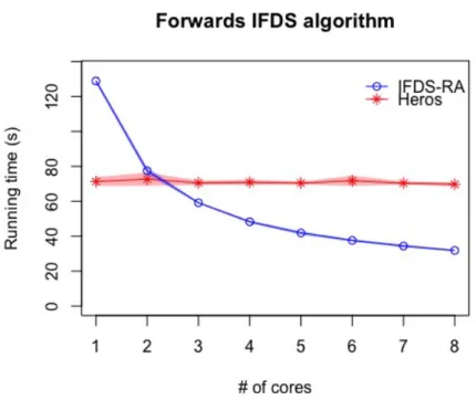
Figure 5.1: Results of test setup 1. The plotted line is the mean of nine execution times and the shaded area around the line is a 95% confidence interval.
CHAPTER 5. RESULTS 27
Table 5.1: Table of mean running time in seconds of test setup 1 and speed-up of IFDS-RA compared to Heros for one to eight cores.
Algorithm 1 2 3 4 5 6 7 8
IFDS-RA 128.90 77.43 59.16 48.28 41.86 37.58 34.41 31.84 Heros 71.32 72.68 70.58 70.91 70.44 71.75 70.40 69.73 Speed-up 0.55x 0.94x 1.19x 1.47x 1.68x 1.91x 2.05x 2.19x
Figure 5.1 shows the experimental results of running the forwards IFDS algorithm on the Java Runtime Environment for both IFDS-RA and Heros for one to eight cores. The analyses ended up reaching 25 sources. The plotted line in the figure is the mean run-ning time of 9 runs and the shaded area is the 95% confidence interval for the runrun-ning time. The running time is stable for both algorithms and as shown in the graph, IFDS-RA shows performance improvements when using multiple cores even if the perfor-mance improvements slows down when using many cores, going from 37 seconds to 32 seconds for six to eight cores compared to 129 seconds to 59 seconds when going from one to three cores. Heros on the other hand performs the same even when using multi-ple cores, showing no improvement.
The exact times can be seen in Table 5.1. The speed-up when using the IFDS-RA al-gorithm compared to the Heros implementation is between 0.94x and 2.19x when using multiple cores.
28 CHAPTER 5. RESULTS
5.2
Test Setup 2
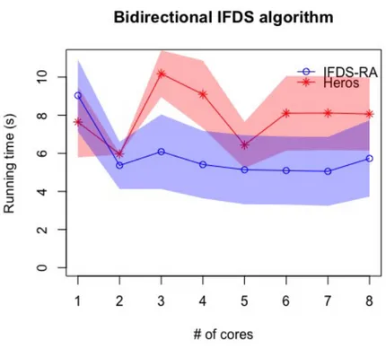
Figure 5.2: Results of test setup 2. The plotted line is the mean of nine execution times and the shaded area around the line is a 95% confidence interval.
Table 5.2: Table of mean running time in seconds of test setup 2 and speed-up of IFDS-RA compared to Heros for one to eight cores.
Algorithm 1 2 3 4 5 6 7 8
IFDS-RA 9.04 5.37 6.09 5.41 5.14 5.10 5.06 5.73 Heros 7.65 5.99 10.18 9.10 6.44 8.10 8.11 8.06 Speed-up 0.85x 1.12x 1.67x 1.68x 1.25x 1.59x 1.60x 1.41x
The results for the second test setup, which used the bidirectional IFDS algorithm, the results can be seen in Figure 5.2. The exact running times and the speed up of IFDS-RA compared to Heros can be found in Table 5.2. The analyses reached 32 sources.
For this test setup, the smaller of the two analyses for the bidirectional algorithm, the results are not clear and the confidence intervals overlap. IFDS-RA seems to show per-formance improvements as the number of cores increase whereas Heros, with exception of cores two and five seems to perform the same even if multiple cores are used. The speed-up of using IFDS-RA compared to Heros on multiple cores is between 1.12x and 1.68x.
CHAPTER 5. RESULTS 29
5.3
Test Setup 3
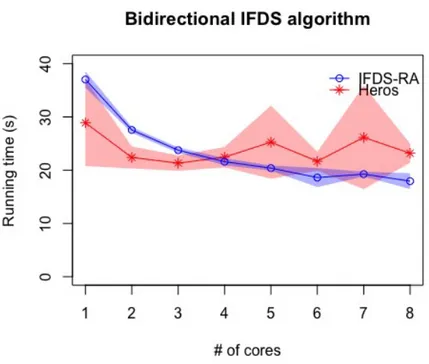
Figure 5.3: Results of test setup 3. The plotted line is the mean of nine execution times and the shaded area around the line is a 95% confidence interval.
Table 5.3: Table of mean running time in seconds of test setup 3 and speed-up of IFDS-RA compared to Heros for one to eight cores.
Algorithm 1 2 3 4 5 6 7 8
IFDS-RA 37.03 27.56 23.76 21.59 20.38 18.62 19.26 17.94 Heros 28.90 22.39 21.33 22.44 25.26 21.67 26.16 23.19 Speed-up 0.78x 0.81x 0.90x 1.04x 1.24x 1.16x 1.36x 1.29x
For the larger test setup using the bidirectional IFDS algorithm, the results can be seen in Figure 5.3. The taint analyses discovered 201 reachable sources. The exact running time and the performance improvements of IFDS-RA compared to Heros can be seen in Ta-ble 5.3. The graphs show the mean running time as a plotted line and a 95% confidence interval as a shaded area around the line.
For this larger, taint analysis, the results are clearer and similar to the first taint anal-ysis. Reactive Async shows a clear trend of performance improvements when using mul-tiple cores. Once again the performance increases slows down when using many cores with a difference of only four seconds between core four and eight. For Heros there is still a lot of variance in the test results but there is no sign that Heros performs better when using multiple cores. In general the speed-up when using IFDS-RA instead of Heros for the third test setup is between 0.81x and 1.36x when using multiple cores.
Chapter 6
Related Work
This chapter presents related work on the IFDS algorithm and how they are similar or different to what has been presented in this paper.
6.1
Concurrent IFDS
This section describes related work on concurrent implementations of IFDS. To our knowl-edge the only other concurrent IFDS solver out there is IFDS-A by Rodriguez and Lhoták [25] mentioned below.
Rodriguez and Lhoták [25] use the actor model [26] to implement a version of the IFDS-algorithm called IFDS-A which can be run in parallel. Similarly to the IFDS-RA al-gorithm presented here, IFDS-A is an extension of the work by Naeem et al. [15]. The implementation of IFDS-A is similar to that of the extended algorithm but utilizes actors to use multiple cores. Each node in the control flow graph is mapped to an actor which internally buffers messages. Messages between actors represent data-flow dependencies. In addition, a tracker keeps track of unprocessed actor messages. When the tracker is zero, the work has been completed and the algorithm can terminate.
The difference between IFDS-A and IFDS-RA is that while both are concurrent ver-sions of the IFDS algorithm, IFDS-RA is based on Reactive Async and IFDS-A is based on the actor model. In addition, instead of having a tracker, as IFDS-A has, for keeping track of when the algorithm is finished, Reactive Asyncs handler pool supports the no-tion of quiescence which means no more work has to be done. This means there is no need to explicitly keep track of this in the algorithm which simplifies the implementa-tion. Also, IFDS-A does not support a bidirectional IFDS algorithm which IFDS-RA does.
IFDS-A is 6.12 times faster using eight cores compared to one core and when using eight cores is 3.35 times faster than a baseline sequential implementation [25].
6.2
Extensions to the IFDS Algorithm
This section describes related work on the IFDS algorithm that is not concurrent. This is presented to give a more detailed view of use cases for the IFDS algorithm and how it can be extended.
CHAPTER 6. RELATED WORK 31
6.2.1 IFDS With Correlated Method Calls
Rapoport et al. [27] transforms an IFDS problem into an interprocedural distribute en-vironment (IDE) problem that precisely accounts for all of the infeasible paths that arise due to correlated method calls. The results of the IDE problem are then mapped back to the original domain of the IFDS problem. This leads to results that are more precise than applying the IFDS algorithm to the original problem. Unlike IFDS-RA, this algorithm is not built for concurrency. Correlated method calls may arise in polymorphism when sev-eral methods are called on the same object whose type is determined at run-time. If a variable can be of type A or type B, any method called on the object will be called on the same object. Therefore, paths that consider the type of the object to be different between two method calls are infeasible.
For a taint analysis this results in a more accurate analysis. Consider an example where A.foo exposes secret information and B.foo, where B inherits from A, does not and B.bar prints the value of foo while A.bar does nothing. There is no way for the secret value in A.foo to be printed by B.bar, they are called on the same object which is of type A or type B. When using the IFDS algorithm directly, a taint analysis would consider this a possibility whereas the work presented in [27] does not.
IFDS-RA could use this technique for a more accurate taint analysis if it adds support for IDE problems which it currently does not have.
6.2.2 Boomerang
Boomerang [28] is a demand-driven pointer analysis based on the IFDS algorithm. Boomerang does two passes of the IFDS algorithm from a given statement, one forward pass and one backward pass. Similarly to IFDS-RA, Boomerang is based on the IFDS im-plementation in Heros presented in [6] with a few extensions. Boomerang is currently single-threaded but a multi-threaded algorithm is currently being developed [28].
The IFDS algorithm is extended by allowing path edges to start from allocation sites and call sites, in addition to a methods entry point like in the IFDS algorithm. This en-ables Boomerang to encode points-to information in the path edges. Boomerang also de-fines three different types of path edges: direct, which represents an allocation site, tran-sitive, which represents a call site, and parameter, which corresponds to the path edge in IFDS used to generate intra-procedural summaries.
The extensions presented in Boomerang could be added to IFDS-RA which is multi-threaded which would result in a multi-multi-threaded version of Boomerang.
6.2.3 T.J. Watson Libraries for Analysis
T.J. Watson Libraries for Analysis (WALA) is a another framework which features an im-plementation of the IFDS algorithm although it is not concurrent. A comparison between the IFDS algorithm in Heros, and WALA, can be found in [6].
The WALA implementation could be used to further strengthen the evaluation of IFDS-RA by comparing it to another IFDS algorithm than Heros.
Chapter 7
Discussion
7.1
Discussion
There are clear performance improvements for IFDS-RA when using multiple cores for the forwards algorithm and for the bidirectional algorithm. The second test setup which showed a lot of variance in the execution times for each core could be because it is a smaller test case and therefore does not run long enough which could explain the varied running time as seen in the confidence interval.
Heros does not improve with multiple cores. This is because of the way its
ThreadPoolExecutoris set up. It is initialized to always use just one thread and queue incoming tasks. This results in a thread pool which does not utilize more than one core. This explains the flat performance of Heros for increasing number of processing cores, it is essentially running the same algorithm for all 8 cores, with no change. However, this diminishes the results of IFDS-RA. It has been shown to scale and perform better than an algorithm which does not scale, which makes the results for IFDS-RA inconclusive and more evaluation is needed to see how it compares to other concurrent IFDS algo-rithms. On the other hand this shows a clear benefit of using Reactive Async, which pro-vides its own pool based on the more modern ForkJoinPool and also demonstrates why an abstraction model such as Reactive Async is useful when dealing with concur-rency. Because Heros outperforms IFDS-RA when using one core, an implementation of Heros which takes advantage of multiple cores could potentially outperform IFDS-RA. However, since Heros uses synchronized block for regular data structures, it might not be the case that it does scale well. The reason Heros outperforms IFDS-RA when using one core could be because it computes the return flow more efficiently by using the edge flow functions which is used to solve IDE problems.
IFDS-RA uses Reactive Async and TrieMaps both of which are lock-free which is a clear improvement over Heros not only in performance but also from a programming perspective. Reactive Async provides an abstraction from threads, locks, and the concur-rency of an application. However, some details still had to be handled outside of Reac-tive Async, for example using TrieMaps for global data structures, this is something that could be improved and replaced with Reactive Async in a future implementation. Even though it would be of interest to replace TrieMaps with Reactive Async, the TrieMaps provide a clear advantage over using regular data structures with locks like Heros does. When iterating over Incoming and EndSummary, as both IFDS-RA and Heros does, Heros locks the data structure and iterates over it to create a local copy which it then iterates