Selected hydrological tools for in-stream flow analysis

Selected Hydrological Tools for In-stream Flow Analysis

Hydrologist. Fort Collins, Colorado 80526

Abstract: The selection of an instream need for a river requires analysis of the riverine hydrology.

Selected tools useful in such an analysis are presented in this paper. Experience in the

determination of an instream flow water right and in the determination of a regulation establishing an instream flow requirement has shown that riverine hydrological analysis must be tailored to the specific river, the riverine ecosystem, and competing water use needs. The riverine hydrological analysis of a specific river most often will include five regimes. These are 1) annual flow regime, 2) high flow regime, 3) low Flow regime, 4) streamflow variation regime, and 5) sediment transport capacity regime. The annual flow regime includes annual runoff and annual maximum discharges. High flows regime includes the time streamflows exceed a selected lower limit on high flows and the selection of the streamflow that is the minimum for high flow needs in a river. The low flow regime includes the frequency of low flows and the number of zero flow days.

Streamflow variation regime considers the variation of streamflows including rapid changes in streamflow. The sediment transport capacity regime considers both the transport of sediment and the maintenance of a channel in a state suitable for a desired ecosystem. The selection of an

analysis year is also considered. In the United States this is October – September (a water year) but other starting and ending months may be more appropriated for a specific river.

1.

Introduction.

Instream flows are an allocation of water to support values obtained from streamflows in a river. The actual allocation of water to instream flows is a policy process. The best situation is when the policy is support by quality analysis of the instream values. The purpose of this paper is to present hydrological analysis tools that are helpful in doing a quality analysis to assist in establishing instream flow requirements for water management purposes. A major purpose of the hydrological analysis is to understand the dynamic characteristics of streamflows in the river or creek without linking the streamflows to the biological system using habitat modeling. Exactly how the results are used depends on the water management situation at hand. The uses of the analysis include 1) comparing

differences in the streamflows between time periods in the measured record such as comparing the streamflow situation prior to a major diversion to the streamflow situation after the diversion, 2) comparing streamflow conditions determined by simulation of alternative water management activities, 3) comparing streamflow conditions resulting from alternative states of the watershed (urban versus rural as an example), and 4) comparing the streamflows at different locations along a river or between rivers.

For the purposes of this paper it is convenient to divide the analysis in to five different regimes of a river. These are 1) annual streamflow regime, 2) high discharge regime, 3) low discharge regime, and 4) sediment transport regime, and 5) flow variability regime. Some of the elements in the various regimes are from Poff (1996) and Richter (1997).

1 _{Hydrologist. Retired US Geological Survey} 1812 Marlborough Court

Fort Collins, Colorado USA

Each of five regimes is briefly described below with an expanded discussion in the following sections.

Annual streamflow regime. The first set of descriptors is descriptors that give information on the annual streamflows in a reach of stream. These include the annual streamflows either described as runoff or as discharge at a point; and the annual maximum

discharges.

High discharge regime. The high discharge regime is an accounting of the magnitude, duration and frequency of high discharges. The analysis requires a ‘high discharge’ to be defined during the analysis.

Low discharge regime. Typical parameters in the low flow regime include the annual values of the minimum 1-day low streamflow in a year, and the minimum of the N-day minimum streamflow. An day streamflow is average over an day period. The N-day period is often 7 N-days. The average annual number of zero flow N-days is an index to the extent of intermittency.

Sediment transport regime. The patterns of sediment transport in a river are of importance in an instream flow analysis. All streamflows are important in the movement of sediment. The length of time of sediment transport is also part of the sediment transport regime.

Flow variability regime. Flow variability is important in understanding the various regimes presented above. Specific factors that characterize streamflow variability include number of adjacent days with an increase in streamflows, number with a decreases, number with no change, indices to streamflow flashiness, and indices to predictability and constancy of the streamflows.

1.1.

Types of data

It is convenient to consider streamflow data to be one of three types as shown in Figure 1. Most instream flow studies use daily streamflow data as a starting point of any

hydrological analysis. The daily data may be from measurements, and data transferred from other locations by various techniques. Watershed models can also be used to

generate streamflows in an ungaged basin. Most recent USGS data is derived from stages measured at 15-minute intervals, transformed to discharges using a rating curve and aggregated to daily values. There are estimated values in most measured daily streamflow data sets, especially for the high and low daily streamflows.

Hydrological Analysis

Data Types

In many rivers the streamflows have been modified by storage, diversions and return flows that have changed over time. If the water management system is relatively simple daily stream flows can be adjusted to a common base period but adjusting daily flows is unlikely to give acceptable results if the system is very complex. In the early days of stream gaging in the United States the only published data available is month streamflows. Also, some water management planning studies use monthly streamflows

Annual streamflows are most often aggregations of daily or monthly values. The annual maximum (peak) discharge is maximum discharge in a year. For most USGS stream gages the peak discharge is the maximum of the 15-minute measurements unless the gage failed in which case the peak may be calculated using a hydraulic model.

1.2.

Example data set.

The river used to illustrate the application of selected hydrological tools is the Pago River near Ordot, Guam (USGS Station 16865000). The following is taken from the US Geological Survey (USGS) description of the gage. The watershed area is 5.57 mi². The period of record is September 1951 to December 1982, September 1998 to current year (2013). The USGS considers the records to be fair, except for estimated periods, which are poor. The average discharge for the period of record of 41 years (water years 1952-82, 1999, 2004-2012) is 25.3 ft³/s (18,350 acre-ft/yr). The Maximum discharge is 17,300 ft³/s, 8 December 2002, gage height, 23.85 ft, from flood marks and rating curve extended above 320 ft³/s on the basis of slope-area measurements at gage heights of 13.22 ft, 15.07 ft, 18.87 ft, and 20.06 ft. Minimum flows are no flow for many days.

All the data used in analysis have been downloaded from the USGS National Water Information System (NWIS) over the last few years. Maps showing the location of the gage and the topography of the watershed may be downloaded from a USGS web site.

1.3.

Selection of a water accounting year

The standard ‘year’ used for water accounting in the United States is the Water Year starting on 1 October and ending on 30 September. This is not always the best period to use for hydrological analysis. The goal of an accounting year is to maximize the

independence of a ‘year’ and the state of the watershed should be as close to the same at the end of each year. In winter snow dominated watersheds this is relatively easy to understand – snow is deposited in the fall and winter and drains out of the watershed in the spring and summer and the watershed returns to a ‘dry’ state at the end of the year.

Another concern is that flood events may be related to a state of the atmosphere which is not the same from year to year. As an example, the southwestern monsoon is a major generator of fall floods in southwestern Colorado some of which occur in the first half of October. The annual southwestern monsoon is one state of the system and the October floods should be included in the year with the same monsoonal state. Consequently, the water accounting year for the Animas River in Colorado and New Mexico should be 1 November – 31 October.

The problem at hand is to define a water accounting year for the Pago River. The first step is to consider the monthly precipitation at a nearby location. In this case the

precipitation gage considered is at Anderson AFB where the average monthly precipitation measured from1 Jan 1953 to 30 Nov 2002 has a minimum monthly value in March. The assumption that a year starts with the water drained out as the rains are reduced (as per snow-melt) suggests the water accounting year should start on 1 April and end on 31 March. 0 2 4 6 8 10 12 14 16

January April July October

Nu m be r of p ea ks in m on th Month

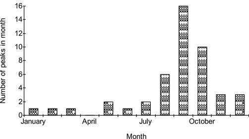
Figure 2. Number days in each month in which the annual maximum discharge occurred in the Pago River

near Ordot, Guam based on water year (1 October - 30 September) data from the peak values files. Data for 1952-1982 and 1999-2012.

The second step is to consider the distribution of the annual peak discharge through the year (see Figure 2). The distribution is based on the annual peak discharges in a US water year. Using a water accounting year starting 1 April is consistent with the distribution of annual peak values.

2.

Annual streamflow regime.

The first set of descriptors is the descriptors that give information on the annual streamflows in a reach of stream. There are two components of the annual streamflows regime. These are the 1) annual streamflows either described as yield from a unit area the watershed (runoff) or as discharge at a point, and 2) the annual maximum (peak) discharge. The annual runoff values are given in Figure 3. The mean annual streamflow of 0.705 m3/s shows the Pago River is a relatively small river and the average runoff of 155 cm shows the watershed, on average, is wet.

0 50 100 150 200 250 300 350 1952 1957 1962 1967 1972 1977 2004 2009 A nn ua l ru no ff, c m

Water accounting year

Figure 3. Annual runoff in the Pago River near Ordot, Guam (USGS Station 16865000). Data is for

1952-1979 and 2004-2012. The watershed area above the gage is 14.4 square kilometers. The water accounting year is from 1 April - 31 March.

The average return periods (frequency) of annual flows can be analyzed using a number of techniques. Three are used herein: 1) duration analysis, 2) assuming a log-normal distribution and 3) assuming a log-Pearson Type III distribution. The results of an analysis of annual streamflows of the Pago River are presented in Table 1. Duration analysis is effectively a graphical technique. For an array ordered from largest to smallest value the equation for the percent equal or larger is:

𝐷_! = 100(!!!.!)_! (1)

where n is the length of the array of annual discharges, m is the location in the array, and Dm is the percent of the discharges equal or larger.

Table 1. Streamflows determined for five return periods and using three alternative calculation techniques

for the Pago River near Ordot, Guam. The annual data is for 1952-1979 and 2004-2013. A year is from 1 April - 31 March. All streamflow values in the table are m3_{/s. Qxx is the annual discharge not exceeded xx} percent of the years.

Q90 Q66.7 Q50 Q33.3 Q10

Duration 1.062 0.751 0.597 0.546 0.464

log-normal 1.024 0.772 0.669 0.579 0.437

log-Pearson

type III 1.039 0.749 0.646 0.565 0.449

The annual maximum discharges can be analyzed using the same techniques.

3.

High discharge regime.

The high discharge regime is an accounting of the magnitude, duration and frequency of high discharges. The definition of a high discharge should be selected based on an

understanding of the reason for a hydrological analysis. The selected discharge is the limiting discharge. The factors describing the high water regime include: 1) median number of days in high water free periods, 2) median number of days in high water

periods, 3) average number of high water periods per year, 4) maximum high water days in 60 day period, and 5) a count of the number of days in each year the discharge exceeds the limiting discharge.

For the Pago River, the limiting discharge for high water periods is the annual

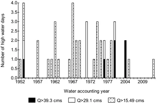
maximum daily discharge exceed once in 1.67 years. The values for the first four factors describing the high water regime are: median number of days in high water free periods is 100, the median number of days in high water periods is 1 (mean of 1.2), the average number of high water per year is 1.16, and the maximum high water days in a 60 day period is 16. The number of days in each water accounting year exceeding three limiting discharges is presented in Figure 4.

0.0 0.5 1.0 1.5 2.0 2.5 3.0 3.5 4.0 1952 1957 1962 1967 1972 1977 2004 2009 Nu m be r of h ig h wa te r da ys

Water accounting year

Q>39.3 cms Q>29.1 cms Q>15.49 cms

Figure 4. Annual number of days the daily discharge exceeds three lower limits in the Pago River near

Ordot, Guam (USGS Station 16865000). Data is for 1952-1979 and 2004-2012. The water accounting year is from 1 April - 31 March.

4.

Low discharge regime

The low flow regime can be characterized by considering the low streamflows in a year as an annual series or by looking at the low streamflows in a seasonal or monthly basis. Typical parameters are the annual values of the minimum 1-day low streamflow in a year, minimum of the 7-day low streamflow, or the minimum of the 10-day streamflow. These can be said to be N-day low flows where N is 1, 7 or 10. An N-day streamflow is average over an N-day period. A singe value of the low streamflow has sometimes been used in instream flow analysis. Often this is the annual N-day discharge with an average return of 1 in 10 years and is abbreviated as NQ10. When N is 7-days this is 7Q10. Some streams have periods of no flow and the average annual number of zero flow days is an index to the extent of intermittency.

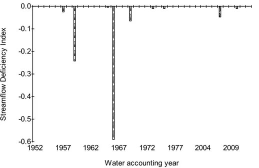
A streamflow deficiency index (QDI) can be used to help understand the frequency and strength of instream droughts. The equation for the index is:

𝑄𝐷𝐼 = _!!!,!{(𝑄 𝑖 − 𝑄_!"#) 𝑄_!"#$  }      𝑄 𝑖 <   𝑄_!"# (2)

where Q(i) is the daily discharge, Qmin is a minimum discharge, and Qmean is the mean

discharge for the river. For the Pago River Qmin was the annual 7-day minimum discharge

not exceeded 1 in 10 years. The annual streamflow deficiency index for the Pago River is given in Figure 5. -0.6 -0.5 -0.4 -0.3 -0.2 -0.1 0.0 1952 1957 1962 1967 1972 1977 2004 2009 St re am flo w D ef ic ie nc y In de x

Water accounting year

Figure 5. Streamflow deficiency Index for the Pago River near Ordot, Guam (USGS Station 16865000).

5.

Sediment transport regime

Water may be the master variable but the water must flow in a stream channel. If the channel is not in adequate condition for a desired ecosystem the water will not have the desired result and be of little value. There are two issues that must be considered 1) can sediment be moved thru the channel with the streamflows available and 2) with a desired condition of the channel be maintained.

The concentrations of suspended sediment as related to discharge is often considered to be a power relation of the form:

𝐶_! = 𝑎𝑄! ₍₃₎

where Cs is the concentration of sediment, Q is the discharge and a and ß are empirical coefficients. For some rivers there may be a critical discharge for sediment movement either because there a low yields from the watershed, the substrate absorbs sediment, or the bed-surface is not disturbed. Consequently, a more general equation is

𝐶_! = 𝑎(𝑄 − 𝑄_!"#)! ₍₄₎

Equation four was used to derive an equation for the Sediment Transport Capacity Index, STCI, shown below:

𝑆𝑇𝐶𝐼 =  

(!_!"#!!_!"#)!!_!"#

!!!,! (5)

where q(i) is the discharge in a period i, and Qref is the reference discharge. Most often the

period is a day and the summation is over the number of days, n, in a year when q(i) is larger than the critical discharge. There are two unknowns: the value of the power term, ß, and the critical discharge. There is little suspended sediment data for the Pago River but there is some data available for a nearby stream, the Ugum River. The data for the Ugum River and the limited data were used estimate the best value of ß is 1.2256 and Qcrt is zero,

Qref was chosen to be 10 m3/s.

These are two goals to be investigated 1) the capacity of the river to transport sediment, and 2) the channel maintenance capacity of the river. In this paper the first goal will be investigated. For second goal see Milhous, 2014. The annual values of the STCI are presented in Figure 6.

0 20 40 60 80 100 120 140 1952 1957 1962 1967 1972 1977 2004 2009 Se di m en t tr an sp or t ca pa ci ty in de x

Water accounting year

Figure 6. Annual sediment transport capacity index for the USGS gaging station on the Pago River near

Ordot on the island of Guam (USGS station 16865000). The water accounting year is 1 April-31 March. Data for 1980-2003 are missing.

The application of the sediment transport capacity and channel maintenance capacity indices requires the determination of the power term, ß, the determination a critical discharge and the selection of a reference discharge. If data is not available good results have been obtained for the STCI using ß equal to 1 and a critical discharge of zero.

6.

Flow variability regime.

Flow variability is important part of all the other regimes. Never the less, there are a number of additional parameters that quantify the variation is streamflows. These include number of rises, number of falls, number with no change, Richards-Baker Flashiness Index, and TQmean. The number of rises is the number of time in a year the daily streamflows increase from day i-1 to day i and the number of falls is the number of times the daily streamflow decreases. The Richards-Baker Flashiness Index (R-BI) is

∑

∑

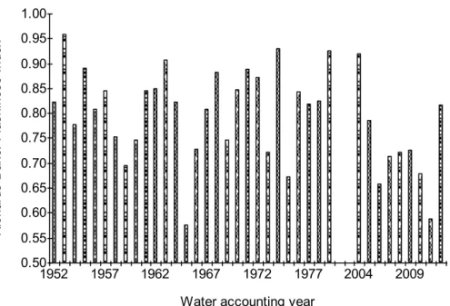
where Q(i) is the discharge in day i. For additional information on the Richards-Baker Flashiness Index see Baker (2004) and for a discussion of TQmean see Booth (2004). The annual variation of the Richards-Baker Flashiness Index in the Pago River is presented in Figure 7.

0.50 0.55 0.60 0.65 0.70 0.75 0.80 0.85 0.90 0.95 1.00 1952 1957 1962 1967 1972 1977 2004 2009 Ri ch ar ds -B ak er F la sh in es s In de x

Water accounting year

Figure 7. Richards-Baker Flashiness Index for the USGS gaging station on the Pago River near Ordot on the

island of Guam (USGS station 16865000). The water accounting year is 1 April-31 March. Data for 1980-2003 are missing.

The Colwell's predictability (P) has been used as an index to the variation in rivers. The index consists of two components Colwell's constancy (C) and Colwell’s contingency (M). The large P the more predictable the streamflows are and the large the total predictability that is constancy (C/P) the more constant the streamflows. The Cowell Index was

calculated for the Pago River using monthly steps and the predictability (P) was found to be 0.379 of which 66.3% is consistence(C). For additional information on the use of Colwell’s Index see Milhous, 2012.

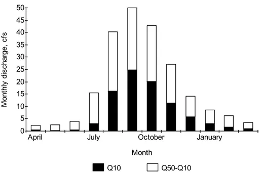
Another form of variability is variation in a time period. This has been used by Richter et al (1997) as a Range of Variability Analysis. The same basic idea had previously been used to look at water availability for allocation to other than instream using monthly streamflows (Chung and Slattery, 1977). This approach is illustrated in Figure 8. The water available for allocation is the difference between a base flow and the monthly streamflow exceeded 1 in 2 years. In Figure 8 the base flow is the monthly discharge not exceeded 1 in 10 years. Chung and Slattery (1977) used another approach to determining the base flow based on daily streamflows.

0 5 10 15 20 25 30 35 40 45 50

April July October January

Mo nt hl y di sc ha rg e, c fs Month Q10 Q50-Q10

Figure 8. Monthly discharge of the Pago River near Ordot, Guam. (USGS station 16865000). Q10 is the

monthly discharge not exceeded 1 in 10 years and Q50 is the discharge exceeded 1 in 2 years.

7.

Discussion

The actual allocation of water to instream uses is a policy process. An understanding of the hydrology of a river is useful in the policy process.

The objective this paper was to present selected hydrological tools that can be used to obtain the information the hydrology of a river to assist in the study of instream flow needs for the river. These include both high and low regimes and the transport of sediment. All are important in the establishment of instream flows.

In this paper no attempt to link the ecosystem to the hydrology has been made because the objective was to show the analytical process. After looking at the hydrology the next step must be to link the ecology of a specific river to the hydrology of the specific river.

References

Baker, D.B., R.P. Richards, T.T. Loftus, and J.W. Kramer. 2004. A new flashiness index: characteristics and applications to midwestern rivers and streams. Journal of the American Water Resources Association 40 (2): 503-522.

Booth, D.B., J.R. Karr, S. Schauman, C.P. Konrad, S.A. Morley, M.G. Laron, and S.J. Burges. 2004. Reviving urban streams: land use, hydrology, biology, and human behavior. Journal of the American Water Resources Association, 40(5):1351-1364.

Chung, Seung K. and Kenneth 0. Slattery. 1977. Colville River Basin. Basin Program Series No. 5. (Water Resources Inventory Area No. 59) Water Resources Management Program. Water Resources

Management Division, Department of Ecology, State of Washington. August 1977. Olympia, Washington 98504

Milhous, R.T. 2012. Application of the Cowell Index to Monthly Streamflow Analysis. J.A. Rameriz, editor. Proceedings, Hydrology Days 2012. Colorado State University. (CD and Web).

Milhous, R.T. 2014. River Morphology as an Element of Environmental Flow Analysis. Proceedsings: 14th Ecohydraulics Symposium (in progress)

Poff, N. LeRoy. 1996. A hydrogeography of unregulated streams in the United States and an examination of scale-dependence in some hydrological descriptors. Freshwater Biology 36: 71-91

Richter B.D., Baumgartner J.V., Wigington R, Braun D.P. 1997. How much water does a river need? Freshwater Biology 37: 231–249.