V¨
aster˚
as, Sweden
Thesis for the Degree of Master of Science in Engineering - Robotics
30.0 credits
VIDEO-RATE ENVIRONMENT
RECOGNITION THROUGH DEPTH
IMAGE PLANE SEGMENTATION FOR
INDOOR SERVICE ROBOT
APPLICATIONS ON AN EMBEDDED
SYSTEM
Ahlexander Karlsson
akn12018@student.mdh.se
Robert Skoglund
rsd12002@student.mdh.se
Examiner: Mikael Ekstr¨
om
M¨
alardalen University, V¨
aster˚
as, Sweden
Supervisor: Fredrik Ekstrand
M¨
alardalen University, V¨
aster˚
as, Sweden
Abstract
As personal service robots are expected to gain widespread use in the near future there is a need for these robots to function properly in a large number of different environments. In order to acquire such an understanding this thesis focuses on implementing a depth image based planar segmentation method based on the detection of 3-D edges in video-rate speed on an embedded system. The use of plane segmentation as a mean of understanding an unknown environment was chosen after a thorough literature review that indicated that this was the most promising approach capable of reaching video-rate speeds. The camera used to capture depth images is a Kinect for Xbox One, which makes video-rate speed 30 fps, as it is suitable for use in indoor environments and the embedded system is a Jetson TX1 which is capable of running GPU-accelerated algorithms. The results show that the implemented method is capable of segmenting depth images at video-rate speed at half the original resolution. However, full-scale depth images are only segmented at 10-12 fps depending on the environment which is not a satisfactory result.
Abbrevations
3-D Three-Dimensional.
AHC Agglomerative Hierarchical Clustering.
BRISK Binary Robust Invariant Scalable Keypoints. CNN Convolutional Neural Network.
CPU Central Processing Unit. D2MC Data-To-Model Coverage. FPGA Field-Programmable Gate Array. FPS frames per second.
GMM Gaussian Mixture Model. GPU Graphics Processing Unit. HMP Hierarchical Matching Pursuit. IR Infrared.
MSE Mean Squared Error.
ORB Oriented FAST and Rotated BRIEF. PCA Principal Component Analysis. PCL The Point Cloud Library. QQVGA Quarter QVGA. QVGA Quarter VGA.
RANSAC RANdom SAmple Consensus. RGB Red, Green, Blue.
RGB-D Red, Green, Blue - Depth. RNN Recursive Neural Network.
SIFT Scale-Invariant Feature Transform.
SLAM Simultaneous Localization And Mapping. SotA State-of-the-Art.
SSIM Structural SIMilarity.
SURF Speeded Up Robust Features. ToF Time-of-Flight.
List of Figures
1 Segmentation example . . . 9
2 An overview of the hardware part of the system. . . 15
3 An overview of the software part of the system. . . 16
4 Depth image with morphological filter . . . 19
5 Visualization of different 3-D edges . . . 20
6 Neighbour arrays . . . 20
7 Distance to line . . . 21
8 Segment and line comparison . . . 23
9 Iterative plane merging . . . 23
10 Plane validation . . . 24
11 Plane merging. . . 25
12 Closing filter on planes . . . 25
13 Effect of depth image downscaling . . . 26
14 D2MC result . . . 28
15 SSIM result . . . 29
16 Full-scale CPU-GPU execution time ratio . . . 30
17 Full-scale edge detection execution time . . . 31
18 Full-scale plane validation execution time . . . 31
19 Half-scale CPU-GPU execution time ratio . . . 32
20 Half-scale edge detection execution time . . . 32
21 Half-scale plane validation execution time . . . 33
22 Appendix: Evaluation of quality on image 1 . . . 44
23 Appendix: Evaluation of quality on image 2 . . . 45
24 Appendix: Evaluation of quality on image 3 . . . 46
25 Appendix: Evaluation of quality on image 4 . . . 47
26 Appendix: Evaluation of quality on image 5 . . . 48
27 Appendix: Evaluation of quality on image 6 . . . 49
28 Appendix: Evaluation of quality on image 7 . . . 50
29 Appendix: Evaluation of quality on image 8 . . . 51
30 Appendix: Evaluation of quality on image 9 . . . 52
List of Tables
1 Result from evaluation of quality . . . 28Contents
1 Introduction 6 1.1 Problem Description . . . 6 1.1.1 Hypothesis . . . 6 1.1.2 Research Questions . . . 6 1.2 Motivation . . . 7 1.3 Contributions . . . 7 2 Background 8 2.1 Hardware . . . 8 2.1.1 Depth Camera . . . 8 2.1.2 Embedded System . . . 8 2.2 Environment Understanding . . . 9 2.2.1 Object Recognition . . . 9 2.2.2 Segmentation . . . 9 2.2.3 Plane Segmentation . . . 10 2.2.4 Semantic Segmentation . . . 102.3 Video-rate Plane Segmentation . . . 11
2.3.1 Local Surface Normals Based Plane Segmentation . . . 11
2.3.2 3-D Edge Based Plane Segmentation . . . 11
2.3.3 Cartesian Voxel Grid Based Plane Segmentation . . . 12
2.3.4 Agglomerative Clustering Based Plane Segmentation . . . 13
3 Method 15 3.1 Hardware . . . 15 3.1.1 Depth Camera . . . 15 3.1.2 Embedded System . . . 16 3.2 Software . . . 16 3.2.1 Environment Understanding . . . 16 3.2.2 GPU Parallelization . . . 17 3.2.3 Programming Language . . . 17 4 Jetson TX1 Setup 18 5 Software 19 5.1 Depth image acquisition . . . 19
5.2 3-D Edge Detection . . . 19 5.2.1 Jump edges . . . 20 5.2.2 Extrema edges . . . 20 5.2.3 Corner edges . . . 21 5.2.4 Curved edges . . . 22 5.3 Plane Candidates . . . 22 5.4 Plane Validation . . . 23 5.5 Plane Merging . . . 24 5.6 Embedded Optimizations . . . 26 6 Evaluation 27 6.1 Quality . . . 27 6.2 Execution . . . 27 7 Results 28 7.1 Evaluation of Quality . . . 28 7.2 Evaluation of Execution . . . 29
7.2.1 Full-scale depth images . . . 30
8 Discussion 34
8.1 Research Questions . . . 34
8.2 Evaluation Result . . . 34
8.3 Kinect for Xbox One issues . . . 35
8.4 Thresholds . . . 35
9 Conclusion 36 10 Future Work 37 10.1 Improvements . . . 37
10.2 Indoor Service Robot Integration . . . 37
11 Acknowledgments 38
References 39
1
Introduction
As personal service robots are expected to gain widespread use in the near future [1] there is a need for these robots to function properly in a large number of different environments. As every home or office presents a different environment these robots must be able to gain an understanding of their surroundings. A robot that can understand an unknown environment without any delay is able to navigate and manipulate this environment in a highly desirable manner.
For an indoor personal service robot application an environment understanding based on depth images can be gained through several different methods. These methods range from just a basic understanding of the geometry of the environment to detailed descriptions of the objects present. It is thus necessary to determine how detailed of an understanding that is necessary for different service robots.
Even though this area of computer vision is well researched within the computer vision com-munity and many solutions to this problem exists there is a lack of focus on solutions that can be used on an embedded system in an actual personal indoor service robot. However, in order for a service robot to function adequately this task must be completed in video-rate on an embedded system.
This master thesis will investigate the state-of-the-art of environment recognition on depth images with the goal of performing the chosen method on an embedded system with video-rate performance.
1.1
Problem Description
In order to properly describe the problem that this thesis aims to solve a hypothesis is formed. This hypothesis is the base for the research questions that this thesis aims to answer.
1.1.1 Hypothesis
By utilizing a Kinect for Xbox One connected to a Jetson TX1 embedded system an indoor service robot can gain an understanding of an unknown environment through plane segmentation. This can be done in video-rate speed and at full depth image resolution by usingGraphics Processing Unit (GPU)-accelerated computing and optimization of a State-of-the-Art (SotA) plane segmentation method for use on the embedded system.
1.1.2 Research Questions
Research Question 1: What hardware is needed in order to run computationally heavy algo-rithms on an embedded system?
In order to achieve video-rate performance there is a need to identify what type of hardware that is necessary based on the performance ofSotAalgorithms onCentral Processing Units (CPUs),GPUs, andField-Programmable Gate Arrays (FPGAs). It is also necessary to eval-uate how powerful the hardware must be in order to process depth images at full resolution in video-rate speed.
As this question is very general it is possible to divide into several more focused questions that are more specifically aimed at the method chosen from from literature review. The first of these more focused research question is:
Research Question 1.1: Is it possible to run the Three-Dimensional (3-D) edge based plane segmentation algorithm on the Jetson TX1GPU andCPU?
If the answer to this research question is true, then the next question is:
Research Question 1.2: At what resolution and at what speed is is possible to run the chosen algorithm?
Research Question 2: How detailed can the understanding of an unknown environment be when running at video-rate speeds on the Jetson TX1 embedded system?
In order to achieve video-rate performance it is impossible to gain an understanding of every detail of the environment. It is thus necessary to limit the amount of detail in exchange for an increase in computational speed. This trade-off must be balanced in order to ensure that an actual understanding of the environment is still obtained.
1.2
Motivation
The critical task of environment understanding is solved by the sensor system of a service robot. One common part of such a sensor system is a computer vision system that is capable of producing depth images of the surrounding environment. A central moment for this vision system is the task of identifying objects and available surfaces in an unknown environment. To solve this problem in an adequate way video-rate environment understanding is the key.
The main motivation behind this thesis is to bridge the gap betweenSotAcomputer vision and service robots. In order for future personal service robots to work properly in varying environments current SotA methods for environment understanding must be used on embedded systems with lower computational power then workstations while maintaining video-rate speeds.
This has not been possible on older embedded systems as the need for parallel computing when it comes to computer vision is high. These embedded systems have lackedGPUsand thus parallel computing architectures such as CUDA1have not been available. Only parallel hardware such as
FPGAshave been suited for parallel computing on embedded systems. However, there are several drawbacks toFPGAsthat make them difficult to work with and this has led to a lack of computer vision methods aimed at embedded systems.
With recent advances inGPU-technology new embedded systems such as the NVIDIA Jetson TX12 have made it possible to utilize the GPU for computer vision on a service robot. This
makes it possible to research howSotAcomputer vision algorithms perform on embedded systems intended for use in indoor service robot applications.
1.3
Contributions
This thesis contributes to the fields of computer vision and service robotics by proving thatSotA
algorithms forRed, Green, Blue - Depth (RGB-D)cameras can be used on embedded systems. It also improves on the chosen method by using a Kinect for Xbox One3camera instead of the Kinect
for Xbox 3604 which means that the method must be adapted in order to facilitate the difference
in the disturbance and accuracy between a Kinect for Xbox 360 and a Kinect for Xbox One.
1CUDA is a parallel programming and computing platform from NVIDIA. http://www.nvidia.com/object/
cuda_home_new.html[Accessed: 30-Jan-2017]
2The NVIDIA Jetson TX1 is an embedded system based around the Tegra X1 chip containing a quad-core ARM Cortex A57 CPU and a 256-core GPU based on the Maxwell architecture developed by NVIDIA. http:
//www.nvidia.com/object/jetson-tx1-module.html[Accessed: 30-Jan-2017]
3Kinect for Xbox One is the latestRGB-Dcamera from Microsoft.https://developer.microsoft.com/en-us/
windows/kinect/hardware[Accessed: 30-Jan-2017]
4Kinect for Xbox 360 is the first version of a RGB-D camera from Microsoft. http://www.xbox.com/en-US/
2
Background
This section is divided into three parts. The first part presents the research done behind the hardware that is used in this thesis and the background to why this hardware has been chosen. The second part presents different approaches to environment recognition, a brief overview of what methods are used to implement them, and how they perform in terms of computation speed with no regards taken to what hardware they are implemented with. This part can be seen as a literature study of theSotAand is used as the basis for what part of this field that is further studied. The last part presents the chosen approach to environment recognition for this thesis and describes the
SotAmethods that achieved video-rate performance in this field in detail.
2.1
Hardware
In order to enable a mobile service robot to gain an understanding of the environment some type of depth vision sensor combined with an embedded system with the capabilities to process the sensor data is needed. This section will describe different solutions to this problem.
2.1.1 Depth Camera
For indoor service robot applications there are two widely used methods that can be used to obtain depth images. The first method is based on RGB-D cameras, such as the Kinect for Xbox One.
RGB-Dcameras work by combining aRed, Green, Blue (RGB)camera with depth data from some type of range sensor. In the case of the Kinect for Xbox One this sensor is aTime-of-Flight (ToF) Infrared (IR) sensor. The other type of camera system that be used in order to obtain depth images are stereo vision systems such as the Bumblebee XB35.
RGB-D cameras are widely used for mobile robot applications as they can be used for a mul-titude of different tasks such asSimultaneous Localization And Mapping (SLAM)[2], object de-tection and tracking [3], and plane recognition [4]. Another advantage is thatRGB-Dcameras are cheap, if two systems of equal performance are compared, and easy to use in comparison to stereo vision systems. The depth from an aRGB-Dcamera come directly from the sensor while the depth from the stereo vision system comes from the calculations performed on the disparity map which is difficult to obtain. When it comes to performance in different environments it is not clear that either solution performs better then the other which can be seen in different comparisons [5, 6]. This heavily depends on the type of environment as the largest drawback of theRGB-D cameras are their relatively limited range. The Kinect for Xbox One has a working range between 0.5 and 4.5 m compared to the working range of stereo vision systems such as the Bumblebee XB3 which can work up 30 meters albeit with severely reduced accuracy. However, for an indoor service robot application a range of 4.5 m is sufficient as indoor areas tend to be relatively small in size. As the Kinect for Xbox One is capable of delivering images at 30frames per second (FPS)this is the speed that video-rate will describe in this thesis.
2.1.2 Embedded System
A mobile service robot platform can not rely on the computational power of a workstation due to size limitations and a need for a low power consumption. Traditionally, embedded system have been lacking the computational power needed to run complex algorithm outside ofFPGA [7, 8] applications as the computation power of embedded systems have been lacking in comparison to workstations. One part of this has been the lack ofGPU-based embedded systems that can be used to massively parallelize demanding software outside of anFPGA. However, new and powerfulGPU -based embedded systems such as the NVIDIA Jetson TX1 have been developed with embedded computer vision as a target. Systems such as this one have made it possible to runGPU-accelerated algorithms on mobile platforms while maintaining the low power consumption that is required. This makes it easier to implemented demanding algorithms for embedded systems as it enables the use of general-purpose programming languages such as C++ instead of the hardware descriptive languages that are necessary forFPGAprogramming.
5The Bumblebee XB3 is a stereo vision camera system developed by Point Grey. https://www.ptgrey.com/
2.2
Environment Understanding
The task of environment understanding can be solved in different ways depending on what infor-mation is deemed important. This section will outline several different methods that can be used to gain this understanding of the environment and at which speeds they can be performed. This study ofSotA methods will be used as a motivation to which approach of environment understanding that this thesis will be focused on.
2.2.1 Object Recognition
One approach that can be used to gain an understanding of the environment is object recognition. This is a widely researched area and there are several different approaches. The two main methods utilize either object descriptors and matching algorithms [9,10] or are based on a type of neural network known as aConvolutional Neural Network (CNN) [11]. [12, Fig. 4] depicts the result of an object recognition system.
The methods based on object descriptors are using established descriptors such as Scale-Invariant Feature Transform (SIFT) [13] and Speeded Up Robust Features (SURF) [14] which are based on histogram of oriented gradients or binary descriptors such as Oriented FAST and Rotated BRIEF (ORB)[15]. By running a combination ofSURF[14] andBinary Robust Invari-ant Scalable Keypoints (BRISK) on aGPU Lee et al. [9] have achieved real-time speeds. New descriptors such as the one proposed by Romero-Gonzalez et al. [10] are outperforming otherSotA
real-value 3D descriptors such as CSHOT [16] in terms of computational speed and scale invariance. However, there is a lack of focus on the computational speed and even though the authors claim real-time performance there is no result showing on whatFPSthey are running the algorithms.
By using a CNN for object recognition high accuracy can be achieved as shown by Wang et al. [11]. By combining a CNN with a descriptor, Li and Cao [17] achieves higher accuracy than
SotA methods such as CNN-Recursive Neural Network (RNN) [18] and Hierarchical Matching Pursuit (HMP)with spatial pyramid pooling [19]. However, the focus with theCNN approach is high accuracy and there is a lack of reported computational times.
Even though an understanding of the environment can be based on object recognition the combination of a lack of reported computational speed and a focus more on specific objects and less on the environment as a whole leads to this approach falling outside the scope of this thesis. 2.2.2 Segmentation
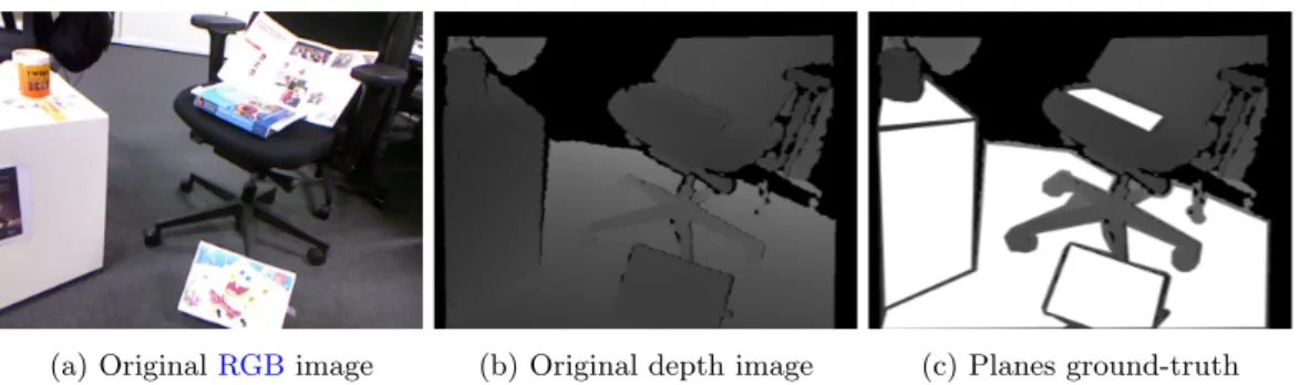
Segmentation is a process that is used to divide an image up into smaller segments where every pixel inside a segment shares the same characteristics. An example of this can be seen in figure1.
(a) OriginalRGBimage (b) Original depth image (c) Planes ground-truth
Figure 1: One example of segmentation from a depth image from the data set used by Javan Hemmat et al. [20].
These segments can then be used in other algorithms in order to gain an understanding of the environment. There exists many different methods that can be used to segment RGB-D
images. Such methods can be based on the Metropolis algorithm [21], the Gaussian Mixture Model (GMM)[22], graph cut theory [23], and a number of other methods.
There are however some differences between these methods. TheGMMbased method focuses on segmenting the foreground from the background. The purpose of this segmentation is to remove
unnecessary information in order to increase the performance of other algorithms focused on areas such as object recognition. Other methods are more focused on segmenting the entire image into coherent parts that can then be further analyzed. Both of these segmentations can be done in video-rate with algorithms running in parallel on aGPUwith the background-foreground segmentation running at 30FPSas shown by Amamra et al. [22] and the coherent part segmentation proposed by Abramov and Pauwels is running between 7 and 111FPS[21] depending on the image resolution. The drawback with segmentation is that it does not provide an environment recognition in itself as the data produced by it must be further processed by other methods. This means that even if the segmentation process can be performed at video-rate speeds it is not guaranteed that the complete environment understanding can.
2.2.3 Plane Segmentation
One segmentation method that can be used to gain at least some understanding of an unknown environment is the segmentation of planar surfaces. An example of this type of segmentation can be seen in [20, Fig. 5]. Important areas of an indoor environment such as floors, walls, and tables are relatively large planar surfaces and thus recognizing these parts leads to an understanding of the environment. With an RGB-D camera this is mainly done with one of many segmentation techniques [4,24, 25, 26,20,27,28,29,30].
This approach to segmentation is commonly known as plane segmentation and a wide variety of methods have been developed using this approach. Video-rate performance running on aCPU
have been met in some of these articles depending on the resolution of the depth images used. The performances range from 7FPSatVideo Graphics Array (VGA)resolution and 30FPSatQuarter QVGA (QQVGA)resolution as shown by Holz et al. [4] and up to 25 FPSat VGAresolution to 130FPSatQQVGAresolution as shown by Wang et al. [29]. One approach to plane segmentation running on either a CPU or a GPU results in 4 FPS when running on the CPU as shown by Hemmat et al. [26] and 100FPSon the GPUas shown by Hemmat et al. [20] atVGAresolution. Frequencies much higher than video-rate performance can thus be achieved when using parallel computing on aGPU. Other plane identification approaches that reaches video-rate performance is a plane extraction approach running at 35FPS atVGAresolution proposed by Feng et al. [25] and a fast plane segmentation running between 2 and 50 FPS at VGA resolution and Quarter VGA (QVGA)resolution as shown by Zhang et al. [30] where video-rate performance is achieved atQVGAresolution. Both of these approaches barely reaches video-rate performance running on aCPU. These approaches have all been evaluated on different data sets containingRGB-Dimages. These data sets are either constructed for the specific approach or are one of several public data sets such as the liris data set [31] and theRGB-D SLAMbenchmark data set [32].
2.2.4 Semantic Segmentation
Another segmentation method that can be used to gain an actual environment understanding is semantic segmentation [33,34,35,36,37,38,39,40,41]. Instead of only identifying planar surfaces this method classifies segments into distinct semantic classes and thus an understanding of objects in the environment is also achieved. An example of this can be seen in [33, Figure 4.]. There are different approaches on how the classification part of this method is performed with some opting for the use of conditional random fields [34, 40] and others support vector machines [37]. Other approaches utilize a combination of both [39]. There are also approaches to this method that includes the use of random forests [38,40,41] or cuboids [35].
Semantic segmentation yields a much deeper understanding of an unknown environment than plane segmentation and thus it would be preferred to semantically segment an unknown area in order to manipulate it with a service robot. However, this approach to environment understanding focuses more on classification accuracy than computational speed. This means that most authors report their performance only in terms of accuracy and there are very few cases where the compu-tation time is shown. The two cases where compucompu-tational speed is reported leads toSotAspeeds between 1.4 FPS, as shown by Wolf et al. [40], and 2 FPS as shown by Wolf et al. [41] which is far from video-rate performance even on non-embedded systems and therefore it is not a suit-able method to use on an embedded system with even lower computational power. Most of these approaches have been evaluated on the NYU version 1 [42] and version 2 [28] data sets.
2.3
Video-rate Plane Segmentation
According to the study ofSotAenvironment understanding techniques presented in the previous section only a few methods that can be used for environment understanding reached video-rate speed. The area with the most methods that did this was plane segmentation and thus it is the chosen area that is explored further in this thesis. There were a total of four methods that reached video-rate speed and this section describes the background in depth for these methods. This background research is used as the basis for the choice of which method that is used in the implementation part of this thesis.
2.3.1 Local Surface Normals Based Plane Segmentation
One approach for achieving video-rate performance plane segmentation is by utilizing local surface normals as proposed by Holz et al. [4]. This approach reaches speeds of approximately 16FPSon
VGAresolution images. These normals are calculated by computing two tangential vectors to the local surface of a point piand calculating the cross product of them. Due to the possibility of noisy
or non-existing depth data from aRGB-D camera in certain regions, a smoothing algorithm that takes the average tangential vectors from the neighborhood is used. The spherical coordinates, (r, φ, θ), are also computed where r is the Cartesian distance between the plane and the origin when it comes to plane segmentation in this method.
The second step of this method is clustering. A normal spaced3-Dvoxel grid is created and the surface normals are mapped to their corresponding grid cell. Each cell containing points above a threshold are considered an initial cluster. These cells are then compared with their neighbors and if two surface normal orientation grids are lower than the cluster threshold and below the desired accuracy the clusters are merged. In order to be able to merge multiple clusters, each merge is saved. This means that a merge of cluster a and b can be compared to a merge of cluster a and c to evaluate which is better.
The third step is to separate each plane into its own cluster. Working with the assumption that every point in a cluster are laying on the same plane the averaged and normalized surface normals are used to calculate the distance from the origin of the plane to the point. The distance will differ for points on a different but parallel plane which is used in order to split the clusters into plane clusters. A logarithmic histogram is used in order to reduce the impact of noise for points further away from the camera.
The final step of this method is used to detect obstacles and objects. This is done by exploiting that both the robot and all objects are either standing on or are supported by horizontal surfaces. All horizontal plane segments are then identified with the help of the camera orientation and extracted. Then aRANdom SAmple Consensus (RANSAC)algorithm [43] is used to optimize and sort out residual outliers from the plane model. This model consists of the average normals and plane-origins in the plane clusters. Then the cluster points are projected onto the plane to calculate the convex hull. This step is then repeated for all relevant horizontal planes. The remaining points that do not exist on a horizontal plane are then investigated. If the point is located both above a planar surface within a certain distance and within that convex hull it is added to that object candidates cluster. If the object candidate does not contain a number of points above a specified threshold it is discarded. When all points have been investigated the centroid and the bounding box of each object candidate is computed. The classification between object and obstacles are done by analyzing their size.
The evaluation of this method is done by comparing the resulted surface normals with the more accurate and computational heavy method of calculating surface normals when the real neighborhood is used withPrincipal Component Analysis (PCA)[44]. The size of the neighborhood linearly depends on the distance from the camera which means that a larger neighborhood is used further away from the camera.
2.3.2 3-D Edge Based Plane Segmentation
Another method that shows video-rate performance is based on the detection of 3-Dedges in a depth image as proposed by Hemmat et al. [20]. This method reaches speeds of almost 100FPS.
The idea behind this method is to use the intrinsic properties that 3-D planes have in order to restrict the searching area to specific areas found between3-Dedges.
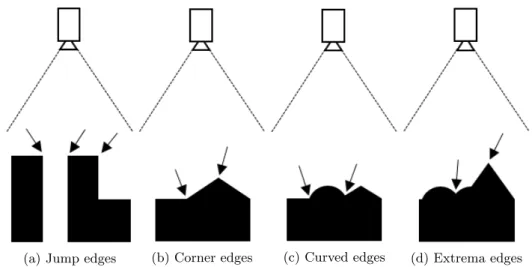
The first step in this method is to detect all edges in a depth image. One important thing to note is that there are several different types of edges that appear in depth images. The four types of edges that are used for this method are jump edges, corner edges, curved edges, and extrema edges. Jump edges are characterized by a sharp increase in the distance from the camera observing the edge. This type of edge occurs when there is a hole in a surface or where there is a gap between two surfaces. Corner edges are found where two planar surfaces meet. Curved edges are found wherever a non-planar surface meets a planar surface. The last type of edge, the extrema edge, is found in local maxima and minima of a surface. It is also important to note that a 3-Dedge can match more then one of these type definitions. For example, a corner edge where two planar surfaces meet can also be an extrema edge if the planes meet in such a way that a local extreme point occurs.
In order to detect these edges some type of edge detection algorithm must be used. However, algorithms that are traditionally used to detect edges in intensity images does not work for depth images. The reason for this is that they only work for edges that display a change in the gray-scale level that can be modeled as a ramp or step while the different types of edges in depth images can not as explained by Coleman et al. [45]. The method used to detect 3-Dedges in this approach scans the image in one pixel wide strips. There are four different strips that are used in this process and they are vertical, horizontal, left-diagonal, and right-diagonal. The different types of edges are then detected by the change of the depth between the pixel in these strips based on the criteria that must be met for an edge to belong to a certain edge-class.
After all edges have been detected the next step is to form candidate planes. This is done by forming one pixel wide strips between the detected edges and traversing these strips in order to determine if they form a line segment or not. This is also done with strips going horizontal, vertical, left-diagonal, and right-diagonal. These line segments are then merged into the candidate planes by merging the points where the line segments intersect. When this step is completed the image has been segmented into planar surfaces but there is still one more step that must be performed in order to validate that the surfaces found are actual planes.
The third and the final step of this methods is the plane validation step. This step is necessary for several reasons. The first one is to verify that the candidate planes are actual planar surfaces. The second is to merge several planar surfaces into one if they are part of the same surface but for some reason divided. This can happen when a planar surface is partially occluded by another object as an example. The third reason for this validation step is to ensure that the detected planes are larger then a minimum size. This validation step can be used in order to filter out small planar surfaces that can be detected on virtually any object or to remove smaller planar surfaces if only large ones such as floors or tables are sought after. The first part of the validation is done by converting the candidate planes into point clouds and calculating the eigenvalues through
PCA. These eigenvalues are then used to determine how curved a surface is and if the result meets a certain threshold the plane is deemed planar. The second part of the validation merges plane candidates by analysis of the normal vectors of the planes that are candidates for merging. The last part of the validation is done by ensuring that the plane candidate contains a specified minimum number of points.
The approach is then validated on a number of data sets collected by the authors. 2.3.3 Cartesian Voxel Grid Based Plane Segmentation
This video-rate performing method, that reaches a speed of 25FPS, is based on creating a voxel grid in the3-DCartesian space and merging plane candidates which have similar normals as proposed by Wang et al. [29].
First theRGB-Dimage is converted into a3-Dpoint cloud. Then a voxel grid is created based on the point cloud. The least squares estimation method is used to approximate a plane utilizing the plane equation containing every point in the voxel. The next step is to cluster the voxels into larger planes. As each voxel now contains a plane candidate, its plane normal is compared to the neighboring voxels plane normal and if they are similar enough they are clustered together. If the size of the cluster is larger then a predefined threshold it is considered to be a plane.
The next step is to refine the plane segmentation by considering the points that do not belong to any of the voxels defining a plane. The area around the voxel is then examined and if no plane is found within a distance r then no point in the voxel is considered to be a part of any plane. However, if a plane is found in the neighborhood of the voxel, then the distance from each point in that voxel to the plane is calculated and if it is lower than a threshold it is considered part of the plane.
The last step of this plane segmentation algorithm is to merge the planes that could describe a larger planar surface. This is achieved by comparing the normal of each plane segment to the plane adjacent to it and if the two normals are similar enough the planes are merged. This step is repeated until every plane segment have tried to merge with its neighbors.
The final part of this method is the detection of obstacles. Working with the idea that obstacles lies on the floor or close to the wall all planes detected are extracted. The larger planes are filtered out and removed from the point cloud as they are considered to be walls or ground, so that all the points remaining in the point cloud are potential obstacles. A similar approach to the coarse plane segmentation in this method is utilized in this part. A voxel grid is constructed and a growing algorithm is used to construct obstacles candidates. If two adjacent voxels contain above a threshold of points they are clustered together and considered to be obstacles.
The evaluation of this method was was done by Wang et al. on the public dataset from [31] and one private dataset and the results were then compared.
2.3.4 Agglomerative Clustering Based Plane Segmentation
The final method that reaches video-rate plane segmentation is based on the line regression algo-rithm [46] but adapted for3-Dusage by Feng et al. [25]. This method achieves speeds of up to 35
FPS. Instead of performingAgglomerative Hierarchical Clustering (AHC)on a double linked list as is the case for 2-D usage the clustering is performed on a planar graph.
The first step of this method is to initialize the planar graph. The point cloud is divided into a number of equally large nodes according to a size set by the user. However, in order for their adaptation of AHC to work properly certain nodes displaying a number of properties must be removed. The first property that leads to the removal of a node is a too high plane fittingMean Squared Error (MSE). The reason for this is that non-planar surfaces have a high plane fitting
MSEand there is thus no reason to use these nodes in order to segment out the planar surfaces as explained by Feng et al.. The second property that leads to node removal is missing depth data. The reason for this missing data is that theIR sensor used inRGB-Dcameras have trouble with objects made from certain materials such as glass. The third property that leads to node removal is depth discontinuity. This occurs when a node contains parts of two surfaces that are not close to each other in3-D space. These nodes are removed due to bad results obtained through thePCA
that is used in the later stages of the method. The fourth property that causes node removal is plane boundaries. If a node contains points that are on two different planes that share a boundary such as a corner it will increase the plane fittingMSEof whichever plane it merges into.
The next step of the algorithm is the AHC. First a min-heap is constructed that contains all the nodes in order to make it easy to find the node with the smallest plane fitting MSE. The node with the lowest plane fittingMSEis then merged with the neighboring node that results in the lowest combined plane fitting MSE. However, if this MSE exceeds a user defined threshold a plane segment is found and removed from the graph. After this process is complete a coarse segmentation of planar surfaces is complete. However, in order to refine this segmentation a final step is performed on the coarse segments.
The end-goal for this step is to remove three types of artifacts that are present after the coarse segmentation. The first artifact that is removed are the jagged edges of the coarse planes that occurs in the boundary regions of the planes. This type of artifact is removed by eroding these regions in order to obtain a smoother edge. The second type of artifact that occurs is unused data points. This is solved by region growing the new boundaries pixel-wise in order to assign all unused points to a plane. The last type of artifact that occurs is oversegmentation. This is solved by utilizing the sameAHCas in the first step of the method in order to combine the oversegmented planes into correctly segmented ones.
3
Method
The work done in this thesis has been based on the engineering design process [48]. The first step of this process is to specify the problem and to gain an understanding of why this problem is important to solve. The second step is the research step. The purpose of this step is to analyze existing methods to gain an understanding of what has been done before. This step leads to a number of possible ways to solve the problem specified and the solution that will be implemented is heavily based on this step. The third step is to propose a solution based on the research followed by an implementation of said solution. This solution is then validated and evaluated. Based on the result some, or all, parts of this process are then iterated in order to refine the final result. This whole process can be summarized as:
• Define the problem
• Conduct background research • Proposal of solutions
• Choose best solution • Implementation • Test and evaluate
• Propose improvements and redesign
3.1
Hardware
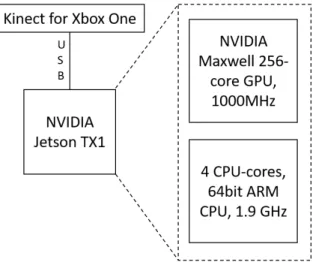
The choice of hardware that is used in this thesis is based on enabling the use of a vision system on an embedded system. The chosen hardware is described in this section along with a motivation to why it has been chosen. The complete hardware set-up can be seen in figure2.
Figure 2: An overview of the hardware part of the system.
3.1.1 Depth Camera
The depth camera that is chosen for this thesis is the Kinect for Xbox One. The main idea behind the choice of anRGB-D camera over a stereo vision system is that theRGB-Dcamera is simpler to work with. The reason for this is that there is no need to perform the same undistortions and rectifications that are needed to obtain the disparity map and in turn the actual distance to objects. The Kinect for Xbox One also works well in indoor environments as this is the environment it is designed to be used in and the same environment that this thesis is aimed at.
3.1.2 Embedded System
In order to be able to test GPU-accelerated algorithms an embedded system with a GPU was required. The main reason for why GPU-accelerated algorithm instead of FPGA-accelerated al-gorithms were the focus of this thesis work is mainly due to the limited time-scope. As GPU -accelerated algorithm can be implemented with general-purpose programming languages instead of hardware descriptive languages the development phase is simplified and thus also shortened and more time can be allocated to background research and proper testing and validation. Another reason for GPU based algorithms over FPGA based ones was that the literature study showed more methods that usedGPUs or had future work that aimed to parallelize the method with a
GPUoverFPGAsand therefore more methods could be investigated.
The NVIDIA Jetson TX1 is an embedded system with a GPU and it is aimed at embedded computer vision and thus it is a good choice for this thesis. It was also available for a reasonable price and different resources such as JetsonHacks6 showed that the Kinect for Xbox One and the
NVIDIA Jetson TX1 were compatible with each other. This compatibility is possible due to it being a Linux based platform and there are already software such as libfreenect2 [49] that can be used to integrate the Kinect with Linux.
3.2
Software
This section will describe the environment understanding method that is implemented in this thesis along with a motivation to why it was chosen. It will also give an overview on how this method is actually implemented in the software.
3.2.1 Environment Understanding
The goal for this thesis is video-rate environment recognition and the literature study showed that the most diverse approach to this problem is plane segmentation. Based on theSotAin this field four methods were further investigated in section2.3. Three of these methods were implemented exclusively on a CPU and even though there are parts of these that can be parallelized they are not designed for it. However, one of the methods have been designed to be run on aGPU
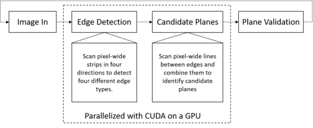
and thus it is deemed to be the most promising solution. This method, 3-D edge based plane segmentation [20], is described in section 2.3.2 and it is displaying a computational speed that is much higher than the 30 FPS that is the target for this thesis. This means that even if the performance lowers significantly due to the reduced computational power of an embedded system video-rate performance can still be achieved. An overview of this method can be seen in figure3.
Figure 3: An overview of the software part of the system.
6Guide on how to use the Kinect for Xbox One with the NVIDIA Jetson TX1. http://www.jetsonhacks.com/
After this method has been implemented it will be evaluated against the same data set that it is originally evaluated on as described by Hemmat et al. [20]. This evaluation will compare the performance of the method when it is running on an embedded system to when it is running on a workstation. An evaluation will also be performed in order to gain an understanding on how the method performs when the input data comes from a Kinect for Xbox One instead of a Kinect for Xbox 360.
Due to the time limitations for this thesis one solution will be focused on during the implemen-tation stage in order to properly implement, validate, and test the solution.
3.2.2 GPU Parallelization
As theGPUon the NVIDIA Jetson TX1 embedded system is an NVIDIA CUDA-enabledGPUthe parallelization is done with the use of CUDA. CUDA enables general-purpose computing on CUDA-enabled GPUs which is used in order to accelerate the parts of the environment understanding methods that are suited for parallel computation.
3.2.3 Programming Language
As CUDA supports C, C++, and FORTRAN one of these languages is thus necessary in order to be able to utilize the GPU to accelerate the chosen method. Due to a lack of knowledge of FORTRAN and the fact that the libfreenect software lacks a FORTRAN wrapper it is out of the question. The instruction videos from NVIDIA that show the basics on how to use the Jetson TX1 platform were helpful during the implementation stage of this thesis and they are showing examples in C++. For this reason C++ is used over C to implement the environment recognition method as it reduced the time that was needed to learn how the system works.
4
Jetson TX1 Setup
The Jetson TX1 used in this thesis is running L4T 24.2.1 as the operating system which is a custom Ubuntu 16.04 version provided by NVIDIA. L4T, along with CUDA Toolkit for Jetson, which contains CUDA 8.0 and OpenCV4Tegra 2.4.13, were installed using Jetpack 2.3.17. Other software and libraries that are used in order to realize the implementation in this thesis is libfreenect2,The Point Cloud Library (PCL)v1.7.2, and Eigen 3.3.38
7JetPack for L4T (Jetson Development Pack) is an on-demand all-one package that bundles and in-stalls all software tools required to develop for the NVIDIA Jetson Embedded Platform.[Accessed: 2017-03-20]https://developer.nvidia.com/embedded/jetpack-2 3 1
8Eigen is a C++ template library for linear algebra: matrices, vectors, numerical solvers, and related algo-rithms.[Accessed: 2017-03-20] http://eigen.tuxfamily.org/index.php?title=Main Page
5
Software
The main part of the 3-D edge based plane detection method is implemented according to the description by Hemmat et al. [20]. This includes the 3-D edge detection, the forming of plane candidates, the plane validation, and the merging of validated plane candidates.
5.1
Depth image acquisition
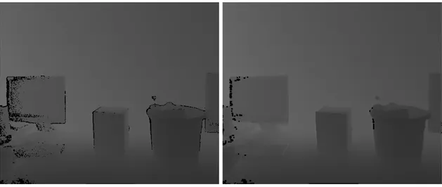
In order to use the Kinect for Xbox One camera on the Linux based Jetson TX1 platform the libfreenect2 software is used. This makes it possible to retrieve depth images from theToFcamera with a resolution of 512x424 pixels. However, due to the characteristics of theToFcamera there will be a number of pixels that lack depth data. This problem mainly occurs on edges of objects and can be seen in the depth image as pepper noise. In order to mitigate this problem where there are only a small number of pixels that lack depth data a morphological filter is applied. This filter, a closing filter, consists of a dilation of the image followed by an erosion. This filter removes parts of the pepper noise, as seen in figure 4, in the depth image that are created due to the lack of depth data.
(a) Unfiltered depth image (b) Filtered depth image
Figure 4: The same depth image shown with and without closing filter. The noise due to missing depth data has noticeably decreased and a more coherent depth image is obtained. Note that the images have been made 16 times brighter for this visualization.
This filtered depth image is then scaled down in order to decrease the computation time. This is done to ensure that the plane segmentation can run at the required 30FPS.
5.2
3-D Edge Detection
The method described by Hemmat et al. defines four different 3-Dedge types that are detected and they are jump edges, corner edges, curved edges, and extrema edges. As these edges occur under different circumstances, as can be seen in figure5, different methods must be used to detect them.
(a) Jump edges (b) Corner edges (c) Curved edges (d) Extrema edges
Figure 5: Illustration of how the four different types of 3-D edges can occur seen perpendicular from the camera view.
However, the first step of these methods, which is the allocation of neighbouring pixels in neighbour arrays according to figure6, is similar in all of them. These neighbour arrays are then used in opposite pairs in order to detect the different edges. The difference is the number of neighbouring pixels that are used. This number depends on a user set threshold that can differ between different edge types. This whole3-Dedge detection is implemented in CUDA in order to parallelize the process.
(a) Vertical (b) Horizontal (c) Left diagonal (d) Right diagonal
Figure 6: An illustration on how the different opposing neighbour arrays are populated during the first step of the3-Dedge detection algorithm. Every square represents a pixel in an array of pixels.
5.2.1 Jump edges
In order to detect jump edges one pixel, the one closest in each direction, is assigned to each neighbour array. A jump edges is then detected if equation1is true. This means that if any pixel in a neighbour array fulfills the criteria the pixel under analysis is a jump edge.
∃p ∈ P : |pdepth− pc
depth| > tje (1)
where: p = Pixel
P = Two opposite neighbour arrays pc = Pixel under analysis
tje= Threshold value for jump edges
5.2.2 Extrema edges
For extrema edges the neighbour arrays are populated with nee pixels each. In order for a pixel
occurs when all pixels in two opposing neighbour arrays are either be larger, or smaller, then the pixel under analysis by an amount dictated by the threshold value.
∀p ∈ P : pdepth> pcdepth∗ tee (2)
∀p ∈ P : pdepth< pcdepth/tee (3)
where: p = Pixel
P = Two opposite neighbour arrays pc= Pixel under analysis
tee= Threshold value for extrema edges
5.2.3 Corner edges
The first step in the corner edge detection is to assign ncoe number of pixels to the neighbour
arrays. Two lines are then formed between the ends of the two neighbour arrays, P1and P2, and
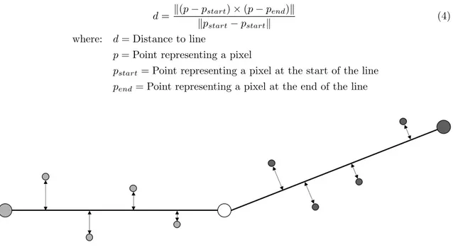
the point that represents the pixel that is under analysis. A point that represents a pixel is defined as (x, y, z) = (column, row, depth). The distance between the other points in a neighbour array and the corresponding line is then calculated according to equation4. This can be seen in figure
7.
d = k(p − pstart) × (p − pend)k kpstart− pstartk
(4) where: d = Distance to line
p = Point representing a pixel
pstart= Point representing a pixel at the start of the line
pend= Point representing a pixel at the end of the line
Figure 7: A visualization of the distance from the points in two opposite neighbour arrays to the lines formed between the end points of a neighbour array and the point that represents the pixel under analysis.
If both equation5and6are true for the calculated distances a third line is formed. This line is formed between the centre points of the two neighbour arrays and the distance is then calculated for every point that is found within this interval. If equation7is true for these distances then the pixel under analysis is a corner edge.
∀p ∈ P1: d < tcoe (5) ∀p ∈ P2: d < tcoe (6) ∀p ∈ P : d > tcoe (7) where: p = Pixel P1= Neighbour array P2= Neighbour array
P = Inner half of P1and P2
d = Distance to line
tcoe= Threshold value for corner edges
5.2.4 Curved edges
Curved edges are detected almost in the same way as corner edges. First two neighbour arrays with ncue pixels are formed. Then two lines are formed between the ends of the neighbour arrays
and the pixel under analysis and the distance between these lines and the corresponding points are calculated. If one, and only one, of equation8 and9is true the third line is formed. The distance for all the points in this interval is then calculated and if equation10is true then the pixel under analysis is a curved edge.
∀p ∈ P1: d < tcue1 (8) ∀p ∈ P2: d < tcue1 (9) ∀p ∈ P : d > tcue2 (10) where: p = Pixel P1= Neighbour array P2= Neighbour array
P = Inner half of P1 and P2
d = Distance to line
tcue1= First threshold value for curved edges
tcue2= Second threshold value for curved edges
5.3
Plane Candidates
The next part of the software forms the plane candidates. This part of the segmentation is also realized on the GPUusing CUDA. The first step in this part is to retrieve all left diagonal and right diagonal pixel segments that are longer than the threshold tlengthand bounded between two
3-D edges. This is visualized in figure8b where left diagonal segments are shown over a depth image with3-Dedges shown as black. These segments are then evaluated with equation4in order to decide if a segment is a line or not which is determined by the threshold tline. A segment is
considered a line if all points on the segment are within a certain distance of the line formed by the start and end point of the segment. The segments that are not considered a line are then removed which can be seen in figure8c.
(a) OriginalRGBimage (b) Left diagonal segments (c) Left diagonal lines
Figure 8: Visualization of the difference between segments and lines in the forming of plane can-didates. Notice how most segments on the trash can, which is a curved surface, are removed after the line evaluation.
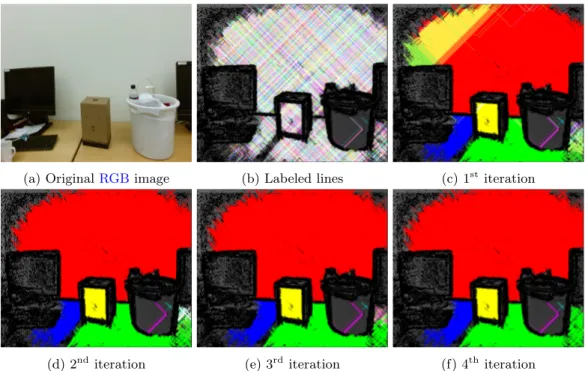
This is done in order to remove segments from non-planar objects such as cylindrical trash cans. Once these lines are established the next step is to label each individual line. Then an iterative merging process is initiated, as seen in figure9, that merges lines that cross each other. Two lines are considered to be crossing each other if they either share a pixel or of they have adjacent pixels.
(a) OriginalRGBimage (b) Labeled lines (c) 1stiteration
(d) 2nditeration (e) 3rd iteration (f) 4th iteration
Figure 9: Visualization of the plane merging process. First all lines are assigned a label. Then every pair of crossing lines is evaluated in parallel and assigned the same label. This process is then repeated until all lines have merged into plane candidates.
5.4
Plane Validation
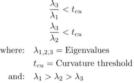
The third step of the3-Dedge based plane detection method is to ensure that the plane candidates are valid planes. In order for a plane candidate to be valid there are two criteria that must be fulfilled. The first is that the plane must be larger than a user defined size tsize. The second is that
the curvature of the plane must be lower than a user defined threshold tcu. In order to evaluate
these two criteria the plane candidates are converted to point clouds. This is done by utilizing
PCL.9If the point cloud then contains more than a user defined number of points the plane is valid 9PCL is a standalone, large scale, open project for 2D/3D image and point cloud processing. http://pointclouds.org/ [Accessed: 13-03-2017]
from a size perspective. In order to validate the curvature of the plane candidate the eigenvalues are used. These eigenvalues are calculated from the point cloud usingPCA. The curvature of the plane is valid if both equation11and 12are true.
λ3 λ1 < tcu (11) λ3 λ2 < tcu (12) where: λ1,2,3= Eigenvalues tcu= Curvature threshold and: λ1> λ2> λ3
This process is visualized in figure10where the planes that are either to small or has a greater curvature than allowed are removed.
(a) Plane candidates before validation (b) Planes after validation
Figure 10: Visualization of the difference between the plane candidates and the actual validated planes. Notice how the plane candidates that are located on the trash can have been removed due to violating both the size and the curvature criteria.
5.5
Plane Merging
The final step of the algorithm is to merge validated plane candidates that belong to the same plane. This is done in order to ensure that a plane that is divided by some occlusion is detected as two parts of the same plane. In order for a merge to occur two criteria must be fulfilled. The first is that the planes must be parallel to each other. The two planes are parallel if equation13
is true.
kn1× n2k < tpar (13)
where: n1= Normal of the first plane
n2= Normal of the second plane
tpar = Parallelity threshold
The second criteria that must be fulfilled is that the two validated plane candidates must lie on the same planar surface. This is done by making sure that the normals for both the planes is perpendicular to the vector that connects the centres of mass of the planes. This is true if equation
n1· γ < tp (14)
n2· γ < tp (15)
where: n1= Normal of the first plane
n2= Normal of the second plane
γ = A vector that connects the centre of mass of both planes tp= Perpendicularity threshold
(a) Validated planes before plane merging. (b) Validated planes after plane merging.
Figure 11: Visualization of the merging of validated planes. The two planes that are detected on the two adjacent tables are merged into one.
After this final step a final post-processing step is applied to the validated and merged planes. This post-processing consists of another morphological filter. If just one pixel is erroneously de-tected as an edge this pixel is never included in any plane candidate. However, for these pixels that lie inside large planes we assume that an erroneous edge has been detected. In order to remove these small empty areas inside the planes a closing filter is applied, as seen in figure12, in order to merge these areas with the plane.
(a) Planes before the closing filter has been applied (b) Planes after the closing filter has been applied
Figure 12: Visualization of the effect of the closing filter on the validated planes. Notice how the small holes in the planes have been filled.
5.6
Embedded Optimizations
In order to use this method on an embedded system, the Jetson TX1, with frame rates at 30FPS
some optimizations had to be done. The largest optimization was scaling down the depth image in order to reduce the number of pixels that has to be processed. The effect of down-scaling the depth image from the Kinect for Xbox One can be observed in figure13. The same planar surfaces are detected even when the image is down-scaled to half the original resolution. However, some details are lost as the detected edges are wider in the down-scaled images in comparison to the full-scale images. This is due to the kernel size, which is as small as possible even for the full-scale images, of the morphological filter that is used on the detected edges in order to close them properly.
(a) Full-scale office (b) Full-scale kitchen (c) Full-scale living room (d) Full-scale bathroom
(e) Half-scale office (f) Half-scale kitchen (g) Half-scale living room (h) Half-scale bathroom
Figure 13: The result of the plane segmentation on both the full-scale and the half-scale depth images.
The other optimization was to move the parts of the algorithms that forms plane candidates from the CPU to the GPU. This meant that a new iterative plane merging algorithm that is able to be used on aGPU was developed. The reason for this optimization is that the original implementation used a dual-layer pipeline where theCPU and GPU parts ran in parallel as the ratio between the execution times were almost 1:1 for the original workstation implementation. In order to maintain a ratio close to 1:1 on the embedded system this optimization had to be done. As there is not enough time to process every frame when running the algorithm on full resolution depth images this ratio enables the highest speed possible. Some other optimizations include the use of OpenCV4Tegra 2.4.13 which is optimized for Tegra use and minor code optimizations compared to the parts of the original implementation, acquired from Hani Javan Hemmat [50], that were used in the paper where Hemmat et al. [20] proposed this method.
6
Evaluation
In order to evaluate this implementation of video-rate plane segmentation of depth images with optimizations for embedded systems an evaluation of the quality and the execution were performed.
6.1
Quality
The quality evaluation of the method in this thesis is done by calculating both the Structural SIMilarity (SSIM)[51,52] and the Data-To-Model Coverage (D2MC), which is the percentage of identical pixels between two images, between a series of nine ground-truth images and the result of the3-Dedge detection and plane segmentation on the same images. These images are a sample data set provided by Hani Javan Hemmat and they are a part of the data set collection that Hemmat et. al used in the evaluation of their implementation [20]. Hani Javan Hemmat also provided the result of their implementation on the same images and theSSIMand D2MCon these images compared to the ground-truth images will be used as the comparison. For theSSIMthe following parameters are used according to the recommendations of the authors of the method; k1 = 0.01,
k2= 0.03, Gaussian window with size according to equation16, L = 255, and a downscaling factor
according to equation16.
F = max(1, round(min(N, M )/256)) (16) where: F = Window size or downscaling factor
N = Number of rows in the image M = Number of columns in the image
One important issue to note is that the depth images in the data set are taken using a Kinect for Xbox 360 and the actual implementation in this thesis used a Kinect for Xbox One. However, this evaluation will be used to validate that the embedded implementation of the method is working correctly.
6.2
Execution
The execution evaluation of the method implemented for this thesis is done by measuring both the time it takes to execute every step of the method and also the time it takes for the whole method. The CUDA kernels will be timed with the cudaEventRecord function while the parts that run on theCPUwill be timed with C++11 <chrono> library.
As the time it takes to process each frame is different depending on how many edges are found, and thus how many segments that are formed, the performance of the algorithm varies between different environments. In order to properly evaluate the performance, in terms of execution speed, of this implementation it will be tested in a number of different environments. These environments range from typical office environments to different home environments such as living rooms and kitchens.
7
Results
This section presents the result from both evaluations performed on the method implemented in this thesis.
7.1
Evaluation of Quality
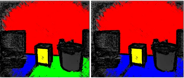
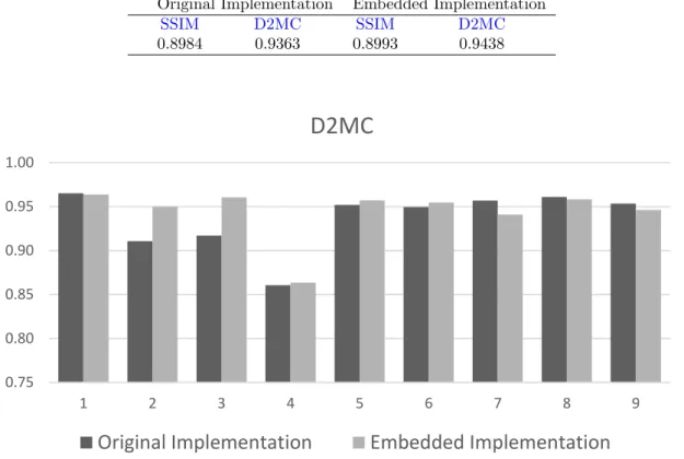
The result from the evaluation of quality can be seen in table 1. This table shows the average value of theSSIMandD2MCon the sample data set. For bothSSIMandD2MCthe higest result possible is one. Thus a value close to one indicates good performance. The result on the individual images can be seen in figure14forD2MCand in figure15forSSIM. The actual segmented planes can be seen next to the corresponding ground-truth in figure22-30in appendixA.
Table 1: Result from evaluation of quality Original Implementation Embedded Implementation
SSIM D2MC SSIM D2MC 0.8984 0.9363 0.8993 0.9438 0.75 0.80 0.85 0.90 0.95 1.00 1 2 3 4 5 6 7 8 9
D2MC
Original Implementation
Embedded Implementation
0.75 0.80 0.85 0.90 0.95 1.00 1 2 3 4 5 6 7 8 9
SSIM
Original Implementation
Embedded Implementation
Figure 15: The result of theSSIMfor every image in the sample data set.
These results were obtain with the following thresholds and number of neighbours: Jump edges: tje= 20
Extrema edges: tee= 0.98, nee= 4
Curved edges: tcue1= 2.9, tcue2= 4, ncue= 12
Corner edges: tcoe= 5.4, ncoe= 16
Plane candidates: tlength= 8, tline= 0.13
Plane validation: tsize= 650, tcu= 0.0325
Plane merging: tpar = 0.03, tps= 0.15
7.2
Evaluation of Execution
The result in terms of average FPS from the execution evaluation can be seen in table 2. All the results presented in this section are an average of the performance of the algorithm over 1800 frames. The time that is not accounted for in the different graphs that are presented when compared to the total execution time is spent on morphological filtering, resizing the depth image, and overhead from theGPUmemory management.
Table 2: AverageFPS
Office Kitchen Living Room Bathroom Half-scale 30.21FPS 30.30FPS 30.26FPS 30.25FPS
The results for full scale depth images were obtained with the following thresholds and number of neighbours:
Jump edges: tje= 60
Extrema edges: tee= 0.98, nee= 4
Curved edges: tcue1= 13.1, tcue2= 3.5, ncue= 8
Corner edges: tcoe= 6.6, ncoe= 16
Plane candidates: tlength= 15, tline= 0.12
Plane validation: tsize= 1000, tcu= 0.0325
Plane merging: tpar= 0.03, tps= 0.15
For the half scale depth images the thresholds and number of neighbours were configured as: Jump edges: tje= 60
Extrema edges: tee= 0.98, nee= 4
Curved edges: tcue1= 4.5, tcue2= 3, ncue= 6
Corner edges: tcoe= 7.5, ncoe= 12
Plane candidates: tlength= 8, tline= 0.3
Plane validation: tsize= 300, tcu = 0.0325
Plane merging: tpar= 0.03, tps= 0.15
7.2.1 Full-scale depth images
Figure16shows the ratio between theCPUandGPUexecution times for full-scale depth images in four different indoor environments. These environments are a generic office environment, a kitchen, a living room, and a bathroom. The ratios for the different environments are 1:2.19, 1:1.89, 1:1.88, and 1:1.82. 35.63 77.94 Full-scale: Office CPU GPU 43.57 82.45 Full-scale: Kitchen CPU GPU 40.53 76.27
Full-scale: Living Room
CPU GPU
42.23 76.74
Full-scale: Bathroom
CPU GPU
Figure 16: Ratio between theCPU and GPU execution times for full-scale depth images. The ratio is not 1:1 but the dual-layer pipeline is still effective even at this ratio. The time presented for each part is in milliseconds.
Figure 17 shows the execution times of the four different edge detection kernels in the four different test environments for full-scale images. The most time consuming edges to detect are corner edges and curved edges.
0 0.05 0.1 0.15 0.2 0.25
Office Kitchen Living Room Bathroom
[ms] Jump Edges 0 0.05 0.1 0.15 0.2 0.25 0.3 0.35 0.4 0.45
Office Kitchen Living Room Bathroom
[ms] Extrema Edges 0 5 10 15 20 25 30 35 40
Office Kitchen Living Room Bathroom
[m s] Corner Edges 0 5 10 15 20 25 30
Office Kitchen Living Room Bathroom
[ms]
Curved Edges
Figure 17: Average execution time for the edge detection of the four different edges in full-scale depth images of four different indoor environments.
In figure18the execution times of the forming of plane candidates and the plane validation on full-scale images are presented. The plane validation part contains both the actual validation of the planes and the final merging of planes.
0 1 2 3 4 5 6 7 8 9 10
Office Kitchen Living Room Bathroom
[m s] Plane Candidates 0.00 5.00 10.00 15.00 20.00 25.00 30.00 35.00 40.00 45.00 50.00
Office Kitchen Living Room Bathroom
[ms]
Plane Validation
Figure 18: Average execution time for the forming of plane candidates and the plane validation and merging in full-scale depth images of four different indoor environments.
7.2.2 Half-scale depth images
Figure19shows the ratio between theCPUandGPUexecution times for half-scale depth images in the four different indoor test environments. The ratios for the test environments for half-scale images are 1:1.85, 1:1.85, 1:1.84, and 1:1.77.
10.02 18.57 Half-scale: Office CPU GPU 10.70 19.76 Half-scale: Kitchen CPU GPU 9.71 17.90
Half-scale: Living Room
CPU GPU
10.73 18.96
Half-scale: Bathroom
CPU GPU
Figure 19: Ratio between theCPUand GPUexecution times for half-scale depth images. While not 1:1 it is close enough to benefit from a dual-layer pipeline. The time presented for each part is in milliseconds.
Figure20shows the execution times of the four different edge detection kernels in the four differ-ent test environmdiffer-ents for half-scale images. For half-scale depth images the most time consuming edges to detect are corner edges and curved edges.
0 0.01 0.02 0.03 0.04 0.05 0.06 0.07 0.08 0.09 0.1
Office Kitchen Living Room Bathroom
[m s] Jump Edges 0 0.05 0.1 0.15 0.2 0.25
Office Kitchen Living Room Bathroom
[ms] Extrema Edges 0 1 2 3 4 5 6 7 8
Office Kitchen Living Room Bathroom
[m s] Corner Edges 0 1 2 3 4 5 6
Office Kitchen Living Room Bathroom
[m
s]
Curved Edges
Figure 20: Average execution time for the edge detection of the four different edges in half-scale depth images of four different indoor environments.
In figure21the execution times of the forming of plane candidates and the plane validation on half-scale images are presented.
0 0.5 1 1.5 2 2.5 3 3.5
Office Kitchen Living Room Bathroom
[m s] Plane Candidates 0.00 2.00 4.00 6.00 8.00 10.00 12.00
Office Kitchen Living Room Bathroom
[ms
]
Plane Validation
Figure 21: Average execution time for the forming of plane candidates and the plane validation and merging in half-scale depth images of four different indoor environments.