Mattias Hjort
Sogol Kharrazi
Olle Eriksson
Magnus Hjälmdahl
Limit handling in a driving simulator
VTI r
apport 861A
|
Limit handling in a driving simulator
www.vti.se/publications
VTI rapport 861A
Published 2015
VTI rapport 861A
Limit handling in a driving simulator
Mattias Hjort
Sogol Kharrazi
Olle Eriksson
Magnus Hjälmdahl
Diarienr: 2011/0510-25
Omslagsbilder: Hejdlösa Bilder AB Tryck: LiU-Tryck, Linköping 2015
Abstract
The purpose of this work has been to investigate how the driving simulator performs at the handling limit of a vehicle and improve its function so that the simulator feels and behaves more like a real vehicle when driving on the limit.
Tests were performed with a Volvo S40, the same vehicle model for which the driving simulator vehicle dynamics model is based upon. Based on these test results the vehicle model that is currently used in VTI’s driving simulator III was modified in order to better simulate vehicle characteristics when driving on the handling limit.
A method for validation of handling characteristics was developed. The method is based on the double lane change manoeuvre, and comprise a subjective and an objective part. The method was regarded to work well, and the validation tests showed that the modified vehicle model closer captures the
understeer and time lag properties of a real Volvo S40 compared to the original model. Still, additional improvements need to be made before the model can be regarded as fully useful for on-the-limit driving situations.
Title: Limit handling in a driving simulator
Author: Mattias Hjort (VTI)
Sogol Kharrazi (VTI) Olle Eriksson (VTI)
Magnus Hjälmdahl Namn (VTI)
Publisher: Swedish National Road and Transport Research Institute (VTI) www.vti.se
Publication No.: VTI rapport 861A
Published: 2015
Reg. No., VTI: 2011/0510-25
ISSN: 0347-6030
Project: Limit Handling
Commissioned by: VTI
Keywords: Limit handling, driving simulator, double lane change, field test
Language: English
Referat
Körsimulatorstudier som involverar körning på gränsen till fordonets förmåga (handling-gränsen) behöver fordonsmodeller som på ett korrekt sätt kan modellera dessa situationer.
Syftet med detta arbete har varit att undersöka hur VTI:s körsimulator presterar vid körning på gränsen till fordonets förmåga och att förbättra dess funktion så att simulatorn i högre grad upplevs och beter sig som ett riktigt fordon i denna situation.
Tester utfördes med en Volvo S40, samma fordon som simulatorns fordonsmodell är baserad på. Utifrån resultaten från dessa tester modifierades fordonsmodellen i VTI:s körsimulator III för att bättre kunna simulera körning på handling-gränsen.
En metod för validering av handling-egenskaper togs fram. Metoden är baserad på double lane change manövern, och består av en subjektiv och en objektiv del. Metoden ansågs fungera väl, och
valideringstesterna visar att den modifierade fordonsmodellen bättre beskriver understyrnings-karakteristik och tidsrespons hos en riktig Volvo S40 jämfört med den ursprungliga modellen. Dock behövs ytterligare förbättringar av modellen innan den kan anses som fullt användbar vid limit handling.
Titel: Limit handling i en körsimulator
Författare: Mattias Hjort (VTI) Sogol Kharrazi (VTI) Olle Eriksson (VTI)
Magnus Hjälmdahl Namn (VTI)
Utgivare: VTI, Statens väg och transportforskningsinstitut www.vti.se
Serie och nr: VTI rapport 861A
Utgivningsår: 2015
VTI:s diarienr: 2011/0510-25
ISSN: 0347-6030
Projektnamn: Limit Handling Uppdragsgivare: VTI
Nyckelord: Limit handling, körsimulator, double lane change, fälttest
Språk: Engelska
Preface
The present study has been initiated and funded by VTI as an internal strategic development project. It has been conducted in order to create increased possibilities and understanding for forthcoming driving simulator studies where modelling of a vehicle at the handling limit is necessary. The project has been carried out by Mattias Hjort and Sogol Kharrazi (the department of Vehicle technology and simulation), Magnus Hjälmdahl (Human-vehicle-transport system interaction) and Olle Eriksson (Infrastructure maintenance).
Other VTI employees that have contributed to the project are Jonas Andersson Hultgren, Fredrik Bruzelius, Erik Olsson, Andreas Jansson, Harry Sörensen, and Sven-Åke Lindén.
Linköping, January 2015
Mattias Hjort Project Manager
Quality review
Review seminar was carried out on 15 December 2014 where Fredrik Bruzelius reviewed and
commented on the report. Mattias Hjort has made alterations to the final manuscript of the report. The research director Jonas Jansson examined and approved the report for publication on 7 May 2015 The conclusions and recommendations expressed are the author’s/authors’ and do not necessarily reflect VTI’s opinion as an authority.
Kvalitetsgranskning
Granskningsseminarium har genomförts 15 december 2014 där Fredrik Bruzelius var lektör. Mattias Hjort har genomfört justeringar av slutligt rapportmanus. Forskningschef Jonas Jansson har därefter granskat och godkänt publikationen för publicering 7 maj 2015. De slutsatser och rekommendationer som uttrycks är författarens/författarnas egna och speglar inte nödvändigtvis myndigheten VTI:s uppfattning.
Innehållsförteckning
Summary ...9 Sammanfattning ...11 1. Background ...13 1.1 Purpose ...13 1.2 Scope ...14 1.3 Work plan ...142 Pre study and method development...16
2.1 The slalom manoeuvre ...17
2.2 The double lane change manoeuvre ...17
2.3 Driving simulator tests ...18
2.3.1 Without motion system ...19
2.3.2 With motion system ...19
2.4 Outcomes of the pre-study ...19
3 The vehicle model ...21
3.1 Existing vehicle model ...21
3.2 Vehicle model “simcar14dof” vs. test data ...22
3.3 Candidate Vehicle Models ...25
3.4 Tyre model ...27
3.4.1 The MF model used in VTI driving simulator ...28
4 Validation at the handling limit ...30
4.1 Validation procedure ...30
4.1.1 Field tests ...30
4.1.2 Driving simulator test ...31
4.2 Subjective evaluation of vehicle behaviour ...32
4.3 Objective evaluation of vehicle behaviour ...32
5 Validation results...33
5.1 Subjective evaluation of vehicle behaviour ...33
5.2 Objective evaluation of vehicle behaviour ...38
6 Discussion and conclusions ...41
References ...43
Appendix I – Equations of the Vehicle Model ...45
Appendix II – Questionnaires ...55
Summary
Limit handling in a driving simulator
by Mattias Hjort (VTI), Sogol Kharrazi (VTI), Olle Eriksson (VTI) and Magnus Hjälmdahl (VTI)
Experiments in driving simulators which study driving and driver behavior close to the vehicle limit demands models that are valid in the non-linear region. With the rapid evolution of active safety systems and semi-autonomous driving systems an increased demand of such experiments is expected. The purpose of this work has been to investigate how the driving simulator, and in particular how the vehicle model, performs at the handling limit of a vehicle and improve its function so that the simulator feels and behaves more like a real vehicle when driving on the limit. Open loop track tests were performed with a test vehicle that is very similar to the one that is modelled in the simulator. Based on these test results the vehicle model currently used in VTI’s driving simulator III was modified in order to better simulate vehicle characteristics when driving on the handling limit. In addition to the original version of the vehicle model, two candidate models were created.
In order to evaluate the effectiveness of applied modifications in the simulator and to compare it to real driving it was also necessary to develop a methodology for performing validations of handling characteristics. The method uses the double lane change manoeuvre, with test drivers performing the manoeuvre first on the test track and then in the driving simulator. The method was divided into a subjective and objective part. The subjective evaluation used questionnaires filled out by the test drivers, while the objective relied on measurements of driver inputs and vehicle response.
It was concluded that subjective evaluation method worked well and did provide useful results. The objective evaluation used a cross correlation method, which provided some valuable insights, but the method needs further improvements for the application considered in this study. One of the main questions in this study was to investigate the fidelity of the timing of the vehicle response in the models, a question that the cross correlation method currently is not able to address.
The validation tests showed that the original vehicle model is more neutral and stable than the real vehicle, and has a too fast response, while resulting in excessive yaw rate. It also lacks the nuances of the real vehicle during the manoeuvre.
In comparison, the new models exhibit some of the nuances of the real vehicle during the manoeuvre, especially for steering response. The yaw rate is also comparable to the real vehicle. However, the vehicle response was too slow during the latter part of the manoeuvre, making the models harder to drive compared to the real vehicle.
This study has helped in understanding how the current vehicle model could be improved for simulating on-the-limit driving, although the method has not yet been fully developed. Both the subjective and the objective parts seems essential for a proper model evaluation. It was shown that the derived vehicle model closer captures the understeer and time lag properties of a real Volvo S40 compared to the original model. Still, additional improvements needs to be made before the model can be regarded as fully useful for on-the-limit driving situations.
Sammanfattning
Limit handling i en körsimulator
av Mattias Hjort (VTI), Sogol Kharrazi (VTI), Olle Eriksson, (VTI) och Magnus Hjälmdahl (VTI)
Körsimulatorstudier som involverar körning på gränsen till fordonets förmåga (handling-gränsen) behöver fordonsmodeller som är valida inom det icke-linjära området. Med den snabba utvecklingen av aktiva säkerhetssystem och autonoma fordon finns ett ökat behov av den typen av studier i framtiden.
Syftet med detta arbete har varit att undersöka hur VTI:s körsimulator, och i synnerhet fordons-modellen, presterar vid körning på gränsen till fordonets förmåga och att förbättra dess funktion så att simulatorn i högre grad upplevs och beter sig som ett riktigt fordon i denna situation. Open loop-tester utfördes med en personbil mycket lik det fordon som fordonsmodellen är baserad på. Utifrån
resultaten från dessa tester modifierades fordonsmodellen i VTI:s körsimulator III för att bättre kunna simulera körning på handling-gränsen. Utöver den ursprungliga fordonsmodellen togs två snarlika kandidatmodeller fram.
För att utvärdera de nya fordonsmodellerna i simulatorn och jämföra den med körning i verklig bil behövde en metod utvecklas för handling-jämförelse vid körning på handling-gränsen. Metoden använder manövern double lane change (dlc) med testförare som utför manövern först på testbana och sedan i simulatorn. Metoden är uppdelad i en subjektiv och objektiv del. Till den subjektiva
utvärderingen används formulär som besvaras av testförarna, medan den objektiva utvärderingen använder sig av mätningar av förarens rattutslag och fordonsrespons.
Den subjektiva utvärderingsmetoden ansågs fungera väl och gav användbara resultat. Den objektiva utvärderingen baserades på en korskorrelationsmetod, vilken gav en del värdefulla insikter, men metoden behöver utvecklas ytterligare för den tillämpning som använts i denna studie. En av huvud-frågorna var hur väl tidsrespons från rattutslag kan modelleras, något som korskorrelationsmetoden inte kan utvärdera i dess nuvarande form.
Valideringstesterna visade att den ursprungliga fordonsmodellen är mer neutral och stabil jämfört med det riktiga fordonet, och har också en för snabb respons och resulterar i för hög girhastighet. Den saknar också en del av de nyanser som det riktiga fordonet uppvisar under manövern.
I jämförelse så uppvisar de nya modellerna några av det riktiga fordonets nyanser under manövern, speciellt när det gäller styrrespons. Girhastigheten är också jämförbar med det riktiga fordonets. Fordonsresponsen är dock för långsam under den senare delen av manövern, vilket gör dess modeller svårare att köra jämfört med det riktiga fordonet.
Denna studie har resulterat i en ökad förståelse för hur den nuvarande fordonsmodellen kan förbättras för simuleringar vid körning på handling-gränsen, även om metoden ännu inte är fullt utvecklad. Både den subjektiva och objektiva delen verkar nödvändiga för en korrekt utvärdering. Sammanfattningsvis så visades att de nya modellerna bättre beskriver understyrningskarakteristik och tidsrespons hos en riktig Volvo S40 jämfört med den ursprungliga modellen. Dock behövs ytterligare förbättringar av modellen innan den kan anses som användbar vid limit handling.
1.
Background
Experiments which study driving and driver behaviour close to the vehicle limit demands reliable models. This is something that we at VTI so far has not studied to a larger extent, and part of the reason is that we are lacking the tools to do so. An example is testing of Active Safety systems, where focus has been on field tests since driving simulators do not perform well enough in situation where the vehicle is close to the handling limit. However, field tests have their share of problems, e.g. repeatability, learning effects, test drivers compared to a population of normal drivers, measurement accuracy etc. Field tests are also often more expensive and suffer from practical problems as weather and road/test track conditions. If it was possible to, in a reliable way, perform such tests in a driving simulator the costs for testing and development could be radically reduced. The quality of measures of driving behaviour with respect to the element of surprise could also be increased, since such tests are very difficult to perform in field due to both practical and safety related problems.
Experiments that compare different constructions of the same system, e.g. FCW (Forward Collision Warning) with haptic or audio warning are not that sensitive with respect to the vehicle model, since they are compared to each other. Typical measures are driver reaction times, which are not directly affected by the vehicle model. Other measures, such as TTC (Time To Collision), minimum headway and TLC (Time to Line Crossing) have not relied on precise vehicle models, since the results for the tested systems are directly compared to each other, and inaccuracies in the vehicle model to a large degree cancel out. The industry has so far not demanded absolute values of the measures, but has been content with the relative performance of different system solutions. However, we foresee a growing demand of absolute measurement values, in order to conclude that a system is good enough, and not only say that system A is better than system B.
The evolution of active safety system is also heading in a direction toward more or less autonomous safety systems, such as Volvo City Safety, auto brake, collision mitigation by braking, collision avoidance by braking/steering. These systems interact either when a collision cannot be avoided and try to reduce damages of the outcome, or at the very last moment when an accident can be avoided by making maximum use the vehicle’s handling properties. To test these systems in a driving simulator, a vehicle model that performs well at the handling limit is required.
We also foresee a number of comfort and eco systems that will require a vehicle model that can perform closer to the vehicle limit than the current model. Examples of such systems are autonomous driving and platooning.
Another example involving situations close the vehicle handling limit would be driving in slippery conditions, or tests of different tyre models. However, before conducting simulator tests involving such situations, the simulator should be validated with respect to its handling properties.
1.1
Purpose
The driving simulators at VTI has not been constructed for on-the-limit driving. We know from experience that for simulations on dry asphalt the driving simulator III is easier to handle during a fast double lane change compared to a standard vehicle in reality. In contrast, for low friction conditions like slippery ice, the simulator may be more difficult to handle compared to a real car. Although the advanced vehicle model in VTI’s driving simulator has not been made for on-the-limit driving, steps in that direction has been taken using simpler models. For example, a diploma work was carried out [The] in 2012 where a simple vehicle model was parameterised and tested in slalom and double lane change manoeuvres.
The purpose of this work has been to investigate how the driving simulator performs at handling limit of a vehicle and improve its function in such situations.
In order to evaluate the effectiveness of applied modifications in the simulator and to compare it to real driving it was also necessary to develop a methodology for performing validations of handling characteristics.
1.2
Scope
It was decided to limit the changes of the driving simulator to the vehicle model. Thus, no
modifications of the motion cueing algorithms, or simulator hardware were considered in this project. Since the vehicle model is the central part of the simulation, it made sense to prioritize that, especially since the model never has been tuned for on-the-limit driving.
Furthermore, it was decided that it would not be possible within the project to conduct a full set of tyre measurements in order to create a new tyre model.
1.3
Work plan
After searching the literature for suitable methods for subjectively and objectively describing vehicle handling properties some initial test drives were conducted in the driving simulator. This resulted in a rough idea for how handling when driving on the limit could be compared for real driving and simulator driving. A work plan consisting of the following points were decided upon:
1. Conduct a pre-study with field tests and driving simulator tests in order to a. Develop the validation methodology
b. Compare the difference between real driving and simulator driving
2. Study the existing vehicle model used in the simulator and identify the model parts that can be improved or parameters that can be adjusted for an enhanced performance at the handling limit
3. Conduct track tests where the vehicle behaviour is measured in various manoeuvres in order to tune the vehicle model in the driving simulator.
4. Tune the vehicle model based on the results from the track test, which should result in a candidate vehicle model that could be compared with the original vehicle model in the validation tests.
5. Perform validation tests where the test drivers are driving a vehicle in limit handling situations on a test track, and then the following day repeat the driving in the simulator comparing both the original and the candidate vehicle model.
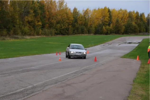
The existing vehicle model represents a Volvo S40 of a model somewhere around year 2000. In order to adjust and validate the vehicle model, a Volvo S40 of year model 2000, was acquired, see Figure 1. It was fitted with new Pirelli P6000 tyres. The vehicle is fitted with ABS (Anti-lock braking system), but does not have ESC (Electronic Stability Control).
Figure 1 - The Volvo S40 of year model 2000 that was acquired for the field tests. (Photo: Mattias Hjort).
The pre-study is described in chapter 2, the track tests and the work with the vehicle in chapter 3, while the validation methodology is described in chapter 4. The results are presented in chapter 5, followed by a discussion and conclusions in chapter 6.
2
Pre study and method development
To get an initial assessment on how the driving simulator compares to real driving in situations close to a vehicle handling limit, a field test at Mantorp Park racing track, followed by simulator drives, was carried out in October 2012. Another purpose of the pre-study was to find out how to describe
handling properties of a vehicle and what questions to ask for subjective evaluation of it. In total 9 test drivers from VTI participated.
Two manoeuvres were tested on wet asphalt: a slalom manoeuvre and a double lane change
manoeuvre. Both manoeuvres are well suited for exploring handling characteristics of a vehicle close to the limit, and are also suitable for simulator implementation. It is known that the vehicle behaviour in both slalom and double lane change is strongly dependent on the vehicle speed. Therefore it was important to note down entry and exit speeds for each test drive. The slalom track was set up so that on-the-limit driving occurred around 60 km/h and the drivers were instructed to drive through it with constant speed if possible.
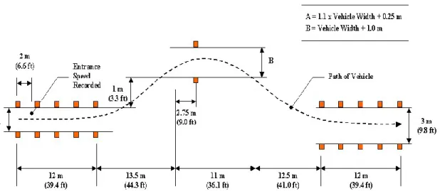
For the double lane change, the modified ISO manoeuvre from NHSTA was used (see Figure 2), which on wet asphalt usually leads to on-the-limit driving at speeds in the range of 55 to 70 km/h. During the double lane change manoeuvre the drivers released the gas throttle and pressed down the clutch at the entry, so that the vehicle coasted down through the manoeuvre; three different phases of the manoeuvre were identified:
1. The entry-section. This represents the first turn to the left by the driver after passing the initial corridor of cones.
2. The mid-section. This phase begins just before the mid cones. The driver must steer to the right to pass the cones and continue steering towards the right lane.
3. The exit-section. The driver needs to steer to the left again to direct the vehicle for the last corridor of cones; while passing them it may be necessary to counter steer in order to avoid skidding.
Figure 2 - The NHTSA modified ISO 3888-2 double lane change course layout. The driver is entering the manoeuvre from the left
It was decided that the following questions should be answered after each manoeuvre:
Does the vehicle understeer/oversteer?
How fast is the steering response?
How much is the degree of perceived control?
In the case of double lane change manoeuvre, the questions were posed for all the three sections (entry, mid and exit). Additionally for the exit section, drivers were asked to specify if a tail swingout occurred and if counter steering was necessary.
2.1
The slalom manoeuvre
The slalom track was set up along a centre line with a distance of 24 metres between each cone. The cones were also diplaced ±0.5 metres from the central line, alternating between left and right of the line. The track was repeatedly wetted to ensure wet track condtions as evident in Figure 3.
Figure 3 - Pre-study field tests: the slalom track (Photo: Mattias Hjort).
General observations from the test drivers were:
Difficult to perform the manoeuvre while keeping up the speed; needs a lot of throttle.
The car is ploughing through the track; heavy understeering. However, with large steering wheel inputs the car can be provoked into oversteer and spinout.
Slow steer response; the steering wheel must be turned a few meters (more than a second) ahead of a cone in order to pass
Difficult to control the vehicle at higher speeds. Around speed of 75 km/h, there is a sudden limit where the car becomes over steered and may result in a spinout. Too much to think about when assessing vehicle behaviour at the same time.
2.2
The double lane change manoeuvre
The cone setup for this pre-study was essentially the same as the NHTSA modified ISO manoeuvre shown in Figure 2. The entry corridor length was reduced for practical reasons, and a car width of 1.75 metres was used. The track was repeatedly wetted to ensure wet track condtions. The drivers drove through the manoeuvre at speeds ranging from 45 to 70 km/h.
Figure 4 - Pre-study field tests: the slalom track (Photo: Mattias Hjort).
General observations from the test drivers for each section were: The entry-section:
The car understeers
The car has a slow steer response; steering should begin early and large steering wheel angle should be used.
The mid-section:
It takes time to change direction of the car The exit-section:
The car responds well
The car does not oversteer much
The car rolls a lot
It is hard to lose control of the car
Furthermore, it was clear that there were too many questions for an unexperienced test driver to answer, for a manoeuvre that only takes about 4 seconds to run through. It was difficult for the driver to register everything; a passenger may be able to assist in answering certain questions, like roll and pitch movement.
2.3
Driving simulator tests
The day after conducting the pre-study field tests the drivers had to drive through the same slalom and double lane change manoeuvres in VTI’s driving simulator III in Linköping. Since the driving
experience could be strongly influenced of the motion queuing algorithms it was decided to perform the test drives in the simulator both with and without motion system activated. All drivers began driving with the motion system deactivated.
A general observation was that most of the drivers started driving in the same way as they had done on the test track, which led to immediate failure. After a while the drivers adjusted their steering inputs and they could better follow the cone tracks.
2.3.1
Without motion system
General impressions from the slalom driving were:
The steer response was much faster in the simulator compared to real driving; it was not necessary to steer as violently as in reality.
It was simpler to perform the maneuverer and control the car.
The car understeered less compared to real driving; it was even oversteering. It felt like the car is steering too much.
The car had too much yaw movement.
It was hard to accurately localize the cones
General impressions from the double lane change were similar to the impressions after driving the slalom manoeuvre, additional observation was that speed reduction in the simulator was much smaller compared to reality. This made it more difficult to control the exit section of the manoeuvre in the simulator; i.e. the car was unstable in the exit section.
2.3.2
With motion system
Activating the motion system changed the impression of the test drivers to some extent. The motion queueing algorithms used for this test were the same as those that are used for normal driving in SIM III. This means that the applied lateral forces in the motion system have been scaled down to 50% of the full simulated force.
General impressions from the slalom driving, which were different from the without motion system case, were:
It was more realistic compared to driving without motion system being activated and it was easier to perform the manoeuvre with activated motion system.
The degree of perceived control was still more compared to real driving.
Activating the motion system made the vehicle feel more understeered
Too large lateral accelerations were felt in the simulator.
Too much roll in the simulator.
For the double lane change tests with the motion system activated, the number of test persons were reduced due to simulator sickness. Still there were some additional impressions from the test drivers, compared to the without motion case:
The go-cart feeling that was present when driving without motion system disappeared; it was not much different from real driving anymore.
The driving experience in the exit section was improved compared to driving without motion system being activated.
2.4
Outcomes of the pre-study
In summary it was concluded that the driving experience in the driving simulator is not too far from the reality when the vehicle is close to its handling limit, however there are differences and the main ones are:
The steer response is faster in the simulator
The car understeers less in the driving simulator
The driver perceives more control over the car, except in the exit section of double lane change manoeuvre, in the driving simulator
The experienced lateral movement is more in the simulator
The experienced retardation is less in the driving simulator
As mentioned earlier, another purpose of the pre-study was to gain knowledge on how to evaluate the driving simulator performance at the handling limit of a vehicle; and to use it as a base for the
methodology development for the main validation study. The main findings are summarized in the following paragraphs.
The comparison results achieved from the slalom and double lane change manoeuvres were quite similar. Thus, considering the limited resources and the problem of excessive tyre wear with long severe manoeuvring on the test track, it was decided to use only one manoeuvre in the main study. Double lane change was chosen due to the fact that it is more representative of the real traffic situations which occur on the road. Furthermore, the double lane change manoeuvre can be divided into three distinct sections, which makes it easier for the drivers to describe their experience during the manoeuvre and rate the vehicle/simulator characteristics in a questionnaire. Another drawback of the slalom test is that it is not easy to keep the speed constant during the manoeuvre.
Since the fast steering response in the simulator was identified as a major issue, it was decided that the driver input (steering wheel angle) and vehicle response (e.g. lateral acceleration and yaw rate) should be recorded during the main validation study, so that the objective comparison of the simulator performance with a real vehicle would be possible.
The gained experience in the pre-study was also used for drafting the questionnaire for the main validation study. It helped to identify the questions which should be asked to capture the main differences between the driving experience in the simulator and in a real car; and to determine questions that are difficult for the test persons to relate to and should be avoided.
Finally, it was also concluded that the simulator study should be performed with activated motion system.
3
The vehicle model
One of the first steps in the project was to study the existing vehicle model used in the simulator and identify the model parts that can be improved or parameters that can be adjusted for an enhanced performance at the handling limit. In the next sections, first the existing vehicle model is described, followed by the description of implemented improvements.
3.1
Existing vehicle model
The existing vehicle model1 represents a Volvo S40 of a model somewhere around year 2000; it is
modelled as a car body (sprung mass) connected to the four wheels via suspension which is represented by a spring-damper assembly at each wheel. The vehicle model has the following 14 degrees of freedom:
Linear planar motion, i.e. longitudinal and lateral motion (2DOF)
Rotations, i.e. roll, pitch and yaw (3DOF)
Vertical motion of the sprung mass (1DOF)
Wheels vertical motion (4DOF)
Wheels rotational speed (4DOF)
Generated forces and moments at the tyre are calculated using the Magic formula (MF) tyre model. The MF parameter set that currently is used in the vehicle model of the driving simulator is the result of the EU project VERTEC, which is further described in section 3.4.1. Each tyre model includes both high and low friction, which in principal could be changed by adjusting the value of the lambda parameter for peak friction.
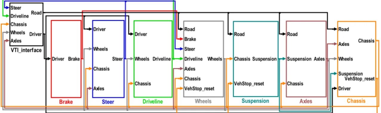
The existing vehicle model is written in FORTRAN and is documented in a report from 1984 (Nordmark 1984) which does not include the applied modifications since then. Due to the difficulties associated with working with the FORTRAN model, it was decided to rebuild the model in Matlab-Simulink within the limit handling project. The resulted Simulink model, referred to as “simcar14dof”, is divided into subsystems to make it more user friendly and easier to work with and modify when necessary, see Figure 5.
Figure 5 - Subsystems of the simcar14dof model in Simulink.
The constituent subsystems of the simcar14dof model are:
Brake: Since the actual brake hardware is available partially in the car cabin, this subsystem is quite simple. The inputs are the brake pressures at each wheel and the outputs are the resulted braking torques.
1 The model is commonly referred to as “Snlib” internally within the FTS group.
Notice: Shake is not included! Road Brake Steer Driveline Axles Chassis VehStop_reset Wheels Wheels Steer Driveline Chassis Wheels Axles Road Driver VTI_interface Road Chassis VehStop_reset Suspension Suspension Driver Wheels Chassis Axles Steer Steer Driver Wheels Chassis Driveline Driveline Road Axles Wheels Suspension Driver Chassis VehStop_reset Chassis Driver Brake Brake Road Suspension Chassis Axles Axles
Steer: The inputs are the driver steering input as well as wheel forces and chassis parameters which are required to calculate the outputs, namely steering angles at wheels and the steering wheel torque felt by the driver.
Driveline: In this subsystem, the engine, gearbox and clutch are modelled. The inputs are the driver inputs (acceleration and clutch pedals and the gear) as well as vehicle speed and wheel rotational speeds. The outputs are driving torque, gear (in case of an automatic gearbox) and engine speed.
Wheels: In this subsystem the rotational speed, longitudinal slip, lateral slip and camber angle of each wheel is calculated and Magic formula tyre model is used to calculate the consequent tyre forces and moments.
Suspension: In this subsystem, the suspension spring, damper and anti-roll bar are modelled; the tyres stiffness is also considered. The inputs are the road surface and chassis parameters such as roll and pitch and the outputs are the resulted suspension forces at each wheel.
Axles: In this subsystem, the axle loads are calculated, using the suspension forces and vehicle accelerations.
Chassis: In this subsystem, the chassis parameters, including longitudinal, lateral, vertical, roll, pitch and yaw motions are calculated. The main inputs are the tyre and suspension forces. More details on the modelled subsystem and the corresponding equations are provided in Appendix I.
3.2
Vehicle model “simcar14dof” vs. test data
The Simulink model was built based on the existing FORTRAN model with rather minor reforms and was validated against the FORTRAN model which showed a good match. For further investigation of the model fidelity, comparison with test measurements were performed. The Volvo S40 test vehicle, described in section 1.3, was equipped with a VBOX data acquisition system, including a GPS receiver and an inertial measurement unit (IMU), which logged signals such as speed, accelerations and yaw rate at a frequency of 100 HZ.
Figure 6 - Sensors to measure steering wheel torque and angle. (Photo: Mattias Hjort).
It was intended to use the VTI steering robot for measuring the steering wheel angle; however, the robot did not fit on the steering column of the Volvo S40. Therefore, a steering wheel sensor for measuring both steering wheel torque and steering wheel angle was developed at VTI measurement lab and mounted on the car, see Figure 6.
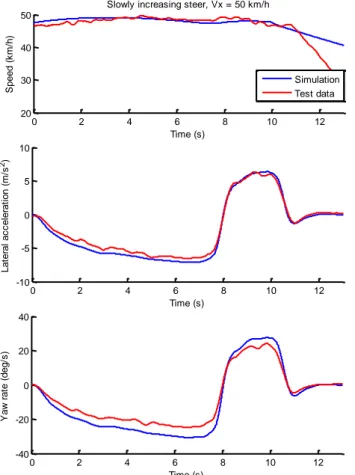
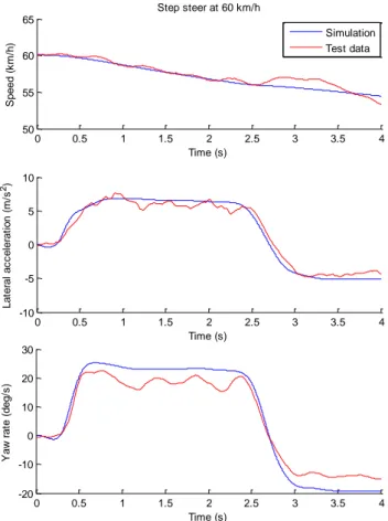
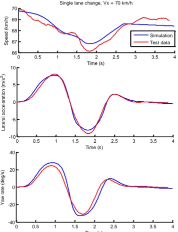
Test manoeuvres were performed on a dry asphalt test track, including step steer, slowly increasing steer and single and double lane changes. The logged steering wheel angle data was used as input to the simcar14dof model, to simulate same manoeuvres. The throttle input in the model was manually adjusted to get similar speed profile during the manoeuvre. The manual tuning approach was chosen over regulating the speed, since it was believed that it will result in a more realistic driving torque pattern with sufficient agreement with the test speed. The comparison results show that the vehicle model is more responsive than the actual car; both lateral acceleration and yaw rate are built up faster in the model. The visual inspection of the yaw rate plots from the actual car and the simulation, indicate a time shift about 50 msec. Furthermore, the peak values of yaw rate, and in some cases the lateral acceleration, are higher in the model compared to the measurements data; the difference is significant for the yaw rate peak, see Figure 7 to Figure 10.
Figure 7 - The simcar14dof model output vs. test data in a slowly increasing steer manoeuvre.
0 2 4 6 8 10 12 20 30 40 50 Time (s) S p e e d ( k m /h )
Slowly increasing steer, Vx = 50 km/h
0 2 4 6 8 10 12 -10 -5 0 5 10 Time (s) L a te ra l a c c e le ra ti o n ( m /s 2) Simulation Test data 0 2 4 6 8 10 12 -40 -20 0 20 40 Time (s) Y a w r a te ( d e g /s )
Figure 8 - The simcar14dof model output vs. test data in a step steer manoeuvre.
Figure 9 - The simcar14dof model output vs. test data in a double lane change manoeuvre.
0 0.5 1 1.5 2 2.5 3 3.5 4 50 55 60 65 Time (s) S p e e d ( k m /h ) Step steer at 60 km/h 0 0.5 1 1.5 2 2.5 3 3.5 4 -10 -5 0 5 10 Time (s) L a te ra l a c c e le ra ti o n ( m /s 2) Simulation Test data 0 0.5 1 1.5 2 2.5 3 3.5 4 -20 -10 0 10 20 30 Time (s) Y a w r a te ( d e g /s ) 0 1 2 3 4 5 6 46 48 50 Time (s) S p e e d ( k m /h )
Double lane change, Vx = 50 km/h
0 1 2 3 4 5 6 -10 -5 0 5 10 Time (s) L a te ra l a c c e le ra ti o n ( m /s 2) Simulation Test data 0 1 2 3 4 5 6 -40 -30 -20 -10 0 10 20 30 Time (s) Y a w r a te ( d e g /s )
Figure 10 - The simcar14dof model output vs. test data in a single lane change manoeuvre.
3.3
Candidate Vehicle Models
Based on the outcome of the comparison of the simcar14dof model outputs with test track measurement, some adjustments were applied to the model.
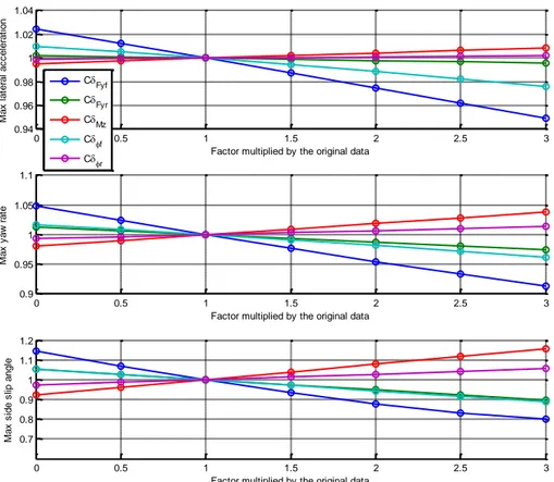
First the sensitivity of model response to some parameters which were expected to have considerable influence on the yaw rate and lateral acceleration were investigated; the considered parameters were: suspension compliance for lateral force (CδFy), suspension torsional compliance (CδMz), roll steer
coefficient (Cδφ), centre of gravity distance from front axle (lf), mass (m) and height of centre of gravity
(hCG). The achieved results for a single lane change manoeuvre at 70 km/h are shown in Figure 11 and
Figure 12.It was concluded that the centre of gravity distance from front axle is the most appropriate parameter to alter, since it can decrease the yaw rate considerably, without affecting the lateral acceleration as much. It should be noted that although the centre of gravity position is relatively easy to measure compared to the other investigated parameters, the purpose of this parameter study was not to quantify the vehicle parameters; but to identify the importance of the correct quantification of a vehicle parameter and its effect on the experienced driving; thus, the position of centre of gravity was altered about 10% to investigate this. To tune the yaw rate response, altering the tyre model parameters were not considered, due to their direct effect on the lateral acceleration which was not desirable.
In order to avoid excessive fast response to the driver steering and to improve the modelled steering system compliance, a first order low-pass filter with time constant of 50 msec was applied to the steering wheel input; the time constant was chosen based on the observed time difference in the vehicle response between reality and simulation. Additionally, the modelled relaxation length of the tyres was adjusted to include the dependency of the relaxation length on the vertical load on the tyre; in the original model a fixed relaxation length is considered. Relaxation length is the distance that a tyre rolls before the lateral force reaches 63% of its steady-state value.
0 0.5 1 1.5 2 2.5 3 3.5 4 66 67 68 69 70 Time (s) S p e e d ( k m /h )
Single lane change, Vx = 70 km/h
0 0.5 1 1.5 2 2.5 3 3.5 4 -10 -5 0 5 10 Time (s) L a te ra l a c c e le ra ti o n ( m /s 2) Simulation Test data 0 0.5 1 1.5 2 2.5 3 3.5 4 -40 -20 0 20 40 Time (s) Y a w r a te ( d e g /s )
Figure 11 - Normalized changes in the maximum lateral acceleration, yaw rate and side slip angle vs. changes in the vehicle parameters.
Figure 12 - Normalized changes in the maximum lateral acceleration, yaw rate and side slip angle vs. changes in the vehicle parameters.
0 0.5 1 1.5 2 2.5 3 0.94 0.96 0.98 1 1.02 1.04
Factor multiplied by the original data
M a x l a te ra l a c c e le ra ti o n 0 0.5 1 1.5 2 2.5 3 0.9 0.95 1 1.05 1.1
Factor multiplied by the original data
M a x y a w r a te 0 0.5 1 1.5 2 2.5 3 0.7 0.8 0.9 1 1.1 1.2
Factor multiplied by the original data
M a x s id e s lip a n g le CFyf CFyr CMz C f C r 0.8 0.85 0.9 0.95 1 1.05 1.1 1.15 1.2 0.9 0.95 1 1.05 1.1 1.15
Factor multiplied by the original data
M a x l a te ra l a c c e le ra ti o n 0.8 0.85 0.9 0.95 1 1.05 1.1 1.15 1.2 0.8 0.9 1 1.1 1.2 1.3
Factor multiplied by the original data
M a x y a w r a te 0.8 0.85 0.9 0.95 1 1.05 1.1 1.15 1.2 0.5 1 1.5 2 2.5
Factor multiplied by the original data
M a x s id e s lip a n g le hCG lf m
The last modification was applied on the lambda parameters of the Magic Formula tyre model to simulate a wet asphalt; as the main validation study, described in Chapter 4, was conducted on a rainy day. Further descriptions are provided in next section.
To conclude, the simulator study was performed with three candidate vehicle models. The original FORTRAN model (model A), the modified Simulink model according to the above described adjustments (model B) and another candidate vehicle model (model C), which only differed from model B by having a smaller time constant (25ms) in the added filter to the steering wheel input. The reason for constructing Model C was that the initial simulations with model B indicated that although it captures the first part of a steering manoeuvre accurately, it results in excessive lag times for following steering inputs.
3.4
Tyre model
For a given pneumatic tyre and road condition, the tyre forces due to slip follow a typical
characteristic. The characteristics can be accurately approximated by a special mathematical function which is known as the "Magic Formula". The parameters in the magic formula depend on the type of the tyre and the road conditions. These parameters can be derived from experimental data obtained from tests. The tyre is rolled over a road at various loads, orientations and motion conditions. The Magic Formula tyre model is mainly of an empirical nature and contains a set of mathematical formulae, which are partly based on a physical background. The Magic Formula calculates the forces (FX, FY) and torques (Mz, MY) acting on the tyre at pure and combined slip conditions, using
longitudinal and/or lateral slip (, ), wheel camber and the vertical force Fz as input quantities. An extension has been provided to also describe transient tyre behaviour. An extensive description of the Magic Formula model can be found in [Pac].
Figure 13 - Magic Formula input and output variables.
Within the description there are separate models describing pure braking and pure steering conditions, resulting in so called slip curves for the forces and torques.
For combined braking and steering, both a longitudinal and a lateral force are generated. These are constructed from the pure slip equations using specific weighing functions.
All the forces described above are steady state forces. In reality, when for example a steering angle is applied on a wheel, the lateral force is not generated immediately. There is a transient behaviour for a few tenths of a second, where the force is built up, which can be described by introducing a relaxation time.
In total some 80 parameters are needed to describe the tyre forces and torques. If a single parameter value is altered, it is impossible to know in advance how this change will affect the generated forces. To allow for a simpler way to change for example the friction level between the tyre and road, an
additional set of parameters was introduced, called the lambda-parameters. Using the lambda
parameters facilitate changes to the slip curves, but may still result in unwanted effects concerning the tyre behaviour in different situations.
3.4.1
The MF model used in VTI driving simulator
The MF parameter set that currently is used in the vehicle model of the driving simulator is the result of the EU project Vertec, which ended 2006. Together with Pirelli, Nokian and other partners, VTI developed MF parameter sets for a passenger car tyre and a heavy truck tyre. Measurements were done on both high friction (dry and wet asphalt, as well as Pirelli’s tyre test machine which uses a sand paper surface) and low friction (ice, done in VTI tyre test facility and snow measured by Nokian). The basic MF parameters of a specific tyre were derived by Pirelli derived from their measurements in the MTS Flat-Trac III machine. Different lambda parameters to be used with this basic MF set were derived from the ice, snow and asphalts measurements. The parameter optimization were all done by Pirelli and were then distributed to all the partners.
For the passenger car tyre model there are both a high and low friction version. For the low friction model the lambda parameters can be changed in order to represent friction level ranging from smooth ice to rough ice and to packed snow. However, this cannot be achieved by only adjusting the value of the lambda parameter for peak friction, since slip curves on ice and snow are qualitatively very different. Instead, a whole number of lambda parameters have to be adjusted for each specific friction level, following a scheme by Pirelli. For the high friction model the lambda parameters were all set to one. VTI is currently using two slightly different models for high friction: one for dry asphalt and one for wet asphalt.
All the measurements at Vårgårda were performed on dry asphalt (it was not allowed to put water on the track since it was also being used as a landing strip for airplanes), and the tuning of the vehicle model was hence performed with the dry asphalt tyre model. The plan was to conduct the validation tests at Mantorp Park also in dry conditions, but unfortunately it was raining during those tests. Thus for the validation tests in the driving simulator it was decided that a wet tyre model should be used. From brake tests performed at Mantorp Park it was seen that the maximum retardation on the wet asphalt during ABS braking was around 7.5 m/s2. This was quite lower than the existing tyre model for
wet asphalt. Thus, for the validation tests a tyre model with lower peak friction than either of the two existing dry and wet asphalt tyre models was needed. Since the dry asphalt model had been used for tuning the vehicle model it was chosen as a basis for a new wet asphalt tyre model. The friction level of the new wet asphalt model was lowered by adjusting the lambda parameters for longitudinal and lateral peak friction coefficient. Since adjusting the tyre model essentially is also an adjustment of the vehicle model itself, it was decided to use the original wet asphalt tyre model when using vehicle model A in the driving simulator, and the new wet asphalt tyre model for model B and C. This decision was made to ensure that model A is representing the driving simulator limit handling
behaviour before the project was carried out. Longitudinal and lateral friction forces at a wheel load of 4000 N for the original and new wet asphalt tyre model are shown in Figure 14
The dry asphalt model has a higher cornering stiffness compared to the original wet asphalt model. Unfortunately, by a mistake the cornering stiffness of the new wet asphalt model was increased an additional 30 percent due to changes in the lambda parameter for slip stiffness. However, for limit handling situations this increased cornering stiffness will likely have only a minor impact on the driving experience since the tyres are mostly in high slip angle region during the performed
manoeuvres and the increased stiffness only affect the tyre lateral force at the linear region where the slip angle is low. Thus, effects of this increased stiffness on the results of the validation tests are expected to be insignificant.
Figure 14 - Longitudinal and lateral slip curves at 4000 N wheel load. Black curves represents original wet asphalt tyre model and red curve the new wet asphalt tyre model.
-1 -0.8 -0.6 -0.4 -0.2 0 0.2 0.4 0.6 0.8 1 -1 -0.5 0 0.5 1 Slip N o rm a liz e d l o n g it u d in a l fo rc e ( F x /F z )
Longitudinal friction force
-30 -20 -10 0 10 20 30 -1 -0.5 0 0.5 1
Slip angle [deg]
N o rm a liz e d l a te ra l fo rc e ( F y /F z )
Lateral friction force
4
Validation at the handling limit
The evaluation aims at verifying that the simulator feels and behaves like a real vehicle when driving on the limit. For this comparison both subjective measurements through questionnaires and objective measurements through data logging in the vehicle. The comparison was made using a double lane change manoeuvre both on a test track and in the driving simulator. 7 drivers were included in the study who drove the car in both experiments. The speed upon entering the manoeuvre was
predetermined and gradually increasing: 55, 60 and 65 km/h. The manoeuvre involved only steering input from the driver. Four repetitions for each speed and driver were carried out.
The number of failed manoeuvres was 7, 8 and 17 in 55, 60 and 65 km/h respectively for the seven drivers on the test track. It showed that the vehicle was on the handling limit already at 65 km/h and there was no reason to try 70 km/h; it would have been beyond the limit and just worn out the tyres.
4.1
Validation procedure
4.1.1
Field tests
The validation tests on the test track was carried out on November 21, 2013 at Mantorp Park racing track. This time we had access to their main straight section, which allowed for a setup on the track where the road surface was essentially flat, as seen in .Figure 15
To record driver input and vehicle response both steering wheel sensor (developed by VTI) and GPS logging at 100 Hz with a VBOX was mounted in the car. An inertial measurement unit (IMU) was also used for measuring accelerations and rotational speeds, see Figure 16.
Figure 16 - Measurement equipment for validation tests: steering wheel sensor (left), VBOX (middle), IMU (right). (Photo: Mattias Hjort).
The drivers worked in pairs with the person not driving sitting in the passenger seat and taking notes according to a predefined schema. Measures of interest are steering response, yaw behaviour and level of control. A few test runs was allowed for the driver to adapt to the car, the surrounding track and the cruise control before the experiment started. The car had a GPS speedometer and the driver had plenty of time to set the cruise control before entering the manoeuvre for the first run and could then press resume to get the same speed in the following runs. The car had manual gearbox and the driver was instructed to clutch down at start of the manoeuvre.
When rating, the driver first drove through the manoeuvre twice according to the procedure described above, then stopped and completed the questionnaire. Then two more runs were carried out and the driver went through the questionnaire again, correcting where necessary. The reason for this procedure was that it forced the drivers to think of the attributes that should be rated, what attributes they were certain about and what attributes needed extra attention during the third and fourth run. If needed the driver could choose to carry out more runs, this was however never needed. In total each driver used roughly 40 – 60 minutes for the field test.
The car was the Volvo S40 described in section 1.3. The air temperature was about +1 C with a mild rain. The asphalt was not new but mostly even with small cracks. The test was made in daylight except for the last driver who finished after the sun had started to set. It should be pointed out that the
temperature was below the ideal, and that the driving was not intense enough to keep the tyres warm. This may have made a direct comparison with the driving simulator more difficult.
4.1.2
Driving simulator test
The driving simulator runs were made the day after the field tests. Each test person drove the simulator with all the three versions of the vehicle model, described in section 3.3, and filled in the questionnaire for each model; the order of the vehicle models was randomised and blind to the drivers. The
evaluation of the simulator behaviour replicated the evaluation of the vehicle as much as possible using the same manoeuvre and the same questionnaire. However, the drivers were alone in the simulator and the simulator questionnaire was complemented with an overall assessment comparing the simulator with the real car with respect to each attribute.
When driving the simulator the driver was not limited to a certain number of runs through the manoeuvre since it does not take as long time to do an extra run in the simulator as on the test track. This meant that the drivers drove a few times until they had a feel for the simulator behaviour, completed the questionnaire, did a few more runs, went through the questionnaire and corrected it where appropriate. The top speed was limited by the simulator to 55, 60 and 65 km/h. The driver
accelerated but could not exceed the pre-set top speed, “declutch” was automatic at entry of the manoeuvre so the driver just let go of the accelerator pedal; automatic gearbox was used during the driving.
4.2
Subjective evaluation of vehicle behaviour
The subjective evaluation was based on the drivers’ ability to rate the vehicles behaviour going
through the double lane change manoeuvre. In order to attend to different aspects of vehicle behaviour, the manoeuvre was divided into three sections: entry, mid and exit. The response was on a nine grade rating scale with five descriptive words on the scale. The reason for using a nine grade scale was that it was of interest to capture small differences when increasing speed and with too few options there was a risk that small differences would not be noted, alternatively that all responses would be at the end of the scale. See Appendix II for the full questionnaire.
In the field test, the rating was done sitting in the car using a pen and paper questionnaire including six different attributes, loosely based on [Pau1]. The attributes were: 1) over- or understeer; 2)
controllability; 3) speed of steering response; 4) possibility to repeat manoeuvre; 5) tail swingout; and 6) effort of steering. For all three sections the driver should rate the vehicle behaviour according to the six attributes above, meaning that for each speed there were 18 different ratings.
The subjective evaluation in the simulator used the same questionnaire as on the test track with the addition of one question in each of the attributes and vehicle models, asking the driver to compare the experience in the simulator to the experience in the real vehicle. This made it possible to observe if the drivers overall impression of the difference between the real vehicle and the models was in line with their more detailed rating of how the vehicle and models behaved. This rating of the overall experience was not separated into entry, mid and exit sections (see Appendix II). The reason for the overall rating was that there was a concern that it would be too difficult for the drivers to perform comparable observations in the field one day and in the simulator the next, given the fact that the drivers are not professional test drivers.
The evaluation is based on mean ratings for the drivers without the use of any inferential statistics. Sample means could be biased because of partial non response and to avoid that, we instead used least squares means when a model was fitted to the available data. The model was a 3-way ANOVA model with driver, speed, section and all 2-factor interactions as explanatory variables.
4.3
Objective evaluation of vehicle behaviour
Three different signals has been studied in the objective analysis. The steering wheel angle has been regarded as the input signal, and the resulting yaw rate and lateral acceleration are output signals. Comparisons of objective measures were carried out following a proposal by [Ste1]. It uses cross correlation as a limit handling parameter, studying the cross correlation between input signal (steering wheel angle) and various output signals such as lateral acceleration and vehicle yaw rate. A time shift is introduced between input and output signal. The time shift resulting in maximum correlation between input and output signals is defined as lag time. The results are then evaluated in terms of maximum correlation and lag times for various speeds. In addition to the cross correlation analysis, the maximum values of steering wheel angle, lateral acceleration and yaw rate during the double lane change manoeuvre in the vehicle and in the simulator (with the three vehicle models) were studied and compared.
5
Validation results
5.1
Subjective evaluation of vehicle behaviour
The analysis of the vehicle field test, as well as the driving simulator test using the three vehicle models, showed that the six attributes could be paired into three groups where the answers to both attributes in that group showed similar pattern. The paired questions in each group are:
Group 1:“Did the vehicle oversteer or understeer?” and “How did you experience the vehicles steering response?”
Group 2:“Did you feel that you had control over the vehicle” and “How did you experience the manoeuvers repeatability”
Group 3: “How much did you experience the tail swingout?” and “How much effort was needed to steer?”
The vehicle models were denoted A, B and C, where model A is the original FORTRAN model, model B the modified Simulink model with 50 ms added time lag, and model C the modified Simulink model with 25 ms added time lag.
The average results from group 1 are shown in Figure 17. A does not understeer as much as the real vehicle does, especially through the midsection. It is more neutral and stays neutral as speed increases while the real vehicle understeers more with higher speed. The steering response is also experienced as quicker for model A. Models B and C, both imitate the behaviour of the real vehicle well with regard to level of under/oversteer, as well as steering response changes with increasing speed.
As shown in Figure 18, drivers felt they have most control over model A. In fact, the controllability of Model A is ranked higher than the real vehicle, especially at low speeds. The tendency for the real vehicle at low speeds was that the feeling of control was reduced through the mid-section and regained again at the exit; this pattern was not seen for model A. For models B and C the feeling of control was much lower already at the low speeds and it seems that the limit is reached already at 55 or 60 km/h, since the control is lost in the midsection and not regained at the exit. For the real vehicle and for models A and C pattern of both control and repeatability is almost unchanged when increasing speed from 55 to 60 km/h, but the controllability and repeatability level decreases at 65 km/h. For model B, this change happens already at speed of 60 km/h.
With respect to tail swingout, model A imitates the real vehicle rather well, but with a little less swingout at the mid-section at 60 km/h, see Figure 19. Models B and C have more tail swingout already at lower speeds and there is little effect of increased speed for model B and no effect of increased speed for model C. This can be explained by the fact that the limit is reached already at 55 km/h.
Higher speed results in an increased effort to steer in all models. The increased effort in A is however not of the same magnitude as for the real vehicle. This is in line with model A having a higher rating on control and being more neutrally steered. Models B and C require more steering effort at low speeds in comparison with the real vehicle. In model C the “effort to steer” curves follow the real vehicle curves but for a 5km/h higher speeds; e.g. the curve for speed of 65 km/h for the real vehicle matches the 60 km/h curve for model C.
One would expect to see similar patterns in the oversteer/understeer graph and the tail swingout graph. This was however not the case, and it seems like the interpretation of understeer/oversteer among the test drivers is how slow/fast the steering response is, which is evident from comparing the graphs in Figure 17.
Of the three models, B and C behaved relatively similar to each other while A differed. Overall the behaviour of model A is more neutral and stable then for the real vehicle. It replicates the real vehicle fairly well but does not have the nuances of the real vehicle, like the increased understeer through the
mid-section. Model B does show some of the nuances of the real vehicle, especially for steering response. There is however a mismatch between the speed – response ratio were model B reaches limit handling at much lower speeds. Model C has, like model B, the nuances of the real vehicle but reaches limit handling at lower speeds. The major results are also summarized in Appendix III.
In an additional question for each attribute in the simulator questionnaire, the drivers were asked for an overall comparison of their experience in the simulator to their experience in the real vehicle. The assessment of this comparison was in line with the difference seen between simulator and real vehicle in the detailed rating.
In the simulator questionnaire, the drivers were asked to compare the experienced lateral motions between the simulator and the real vehicle by checking one of nine boxes ranging from "Much more powerful" to "Much less powerful". The drivers experienced that the lateral motions in the simulator was slightly more powerful than in the real vehicle, on average one scale step away from the neutral alternative on this nine grade scale. The drivers rating did not depend on the speed. The lateral forces in the motion cueing of the simulator are scaled down to about 50 % as mentioned in section 2.3.2, but the drivers respond to this question indicate that there might be a need for further reduction of lateral forces.
Figure 17 - Subjective evaluation of “oversteer/understeer” and “steering response”. The dashed lines in the lower plots are the field test results.
Figure 18 - Subjective evaluation of “controllability” and “repeatability”. The dashed lines in the
Figure 19 - Subjective evaluation of “tail swingout” and “Effort to steer”. The dashed lines in the lower plots are the field test results.
5.2
Objective evaluation of vehicle behaviour
As described in section 4.3, three different signals were studied for the objective evaluation of the vehicle and models behaviour at handling limit. The steering wheel angle (SWA) has been regarded as the input signal, and the resulting yaw rate and lateral acceleration are output signals. Comparisons of objective measures were carried out using cross correlation as a limit handling parameter, studying the cross correlation between input signal and the output signals, after introducing a time shift between them. The time shift resulting in maximum correlation between input and output signals is defined as lag time. The results were then evaluated in terms of maximum correlation and lag times for various speeds.
Figure 20 shows the recorded steering wheel angle and yaw rate from a single field test drive. From visual inspection of the curves the time lag between input and output signal seems to be about 0.10 sec throughout most of the manoeuvre. However, there is a discrepancy during the exit section of the manoeuvre when the driver tries to straighten up the car and the time lag is closer to 0.05 sec (occurs between 3.0 and 3.5 sec in the graph).
Figure 20 - Steering wheel angle (SWA) and result ng yaw rate in field test and simulations from a single field test drive at 60 km/h.
When the recorded steering wheel angle is run through the three vehicle models the resulting yaw rate curves exhibit a different behaviour. It is clear from the figure that model A is too responsive during the first turn of the manoeuvre, while models B and C are closer to the field test data. On the other hand, during the mid-section when the driver begins to steer back, model A is now in phase with the field test data, while B and C are too slow. Which model that is closest to reality changes along the time line, and it is clear that neither of them accurately captures the dynamics of the manoeuvre. This non-constant time lag effect may pose a problem when using the cross correlation method with a constant time lag for comparing the models.
In Figure 21 the maximum values of the steering wheel angle, lateral acceleration and yaw rate is shown for each test drive – field tests and driving simulator tests combined. It is clear that the peak lateral acceleration level of model A better represents the actual field test conditions in comparison with models B and C. The reason for this could be that the peak friction level of the new wet tyre model was set a bit too low; in addition the changes made to the vehicle model for tuning the yaw rate response, also lowers the lateral acceleration that can be achieved.
Furthermore, maximum steering inputs are bigger for models B and C, while model A better
represents the field tests, which is not surprising considering that model A is more responsive. On the other hand, inspection of the maximum yaw rate shows that models B and C are well in line with the
0 1 2 3 4 5 6 -40 -30 -20 -10 0 10 20 30 40 Time (s) Y a w r a te ( d e g /s ) Field test Sim Model: A Sim Model: B Sim Model: C SWA / 4
field tests, while model A results in far excessive yaw rate. In essence, models B and C have a general understeer behaviour that is closer to the real vehicle, which is also evident from the subjective evaluation.
Figure 21 - Comparison of field tests and simulator tests: maximum absolute values of steering input, lateral acceleration and yaw rate.
Figure 22 - Comparison of field tests and simulator tests: Correlation between input signal (swa) and output signals (yaw rate and lateral acceleration).
The dynamics of the different models compared to the field tests is evaluated using the cross
correlation method; the results are shown in Figure 22. It is clear that for the field tests the correlation between input and output signals is quite high for the lower speed, but becomes increasingly worse as the speed is getting higher, particularly for the yaw rate. Since the correlation method does not seem to be useful for situations where the vehicle is close to the handling limit even for the field tests, the method should be revised or complemented with an additional evaluation tool.
The general impression is that the driving simulator models have lower correlation values than the field test. Particularly model A shows low correlation for lateral acceleration during the limit handling conditions at 65 km/h. 50 55 60 65 70 0 100 200 300 400 500 600 Speed (km/h) S W A ( d e g )
Max steering wheel angle
50 55 60 65 70 0 2 4 6 8 10 Speed (km/h) L a t a c c e le ra ti o n ( m /s 2)
Max lateral acceleration
field test Sim Model: A Sim Model: B Sim Model: C 50 55 60 65 70 0 20 40 60 80 100 Speed (km/h) Y a w r a te ( d e g /s )
Max yaw rate
50 55 60 65 70 0.5 0.6 0.7 0.8 0.9 1 Speed (km/h) C o rr e la ti o n
correlation yaw rate
field test Sim Model: A Sim Model: B Sim Model: C 50 55 60 65 70 0 0.1 0.2 0.3 0.4 0.5 Speed (km/h) T im e s h if t (s )
Time shift yaw rate
50 55 60 65 70 0.5 0.6 0.7 0.8 0.9 1 Speed (km/h) C o rr e la ti o n
correlation lat acc
50 55 60 65 70 0 0.2 0.4 0.6 0.8 Speed (km/h) T im e s h if t (s )
It can be concluded that the cross correlation method can be useful, but needs to be tailored for the application considered in this study. This is due to the fact that the time shift between input and output signals is not constant during the double lane change manoeuvre, complicating the evaluation. One possible solution is to divide the manoeuvre into sections with piecewise constant time lag and utilize the cross correlation method on the individual sections. However, more work is needed to verify this. One of the impressions from the pre-study was that the speed reduction was too low in driving simulator, which would make the manoeuvre more difficult to pass. However, comparing the speed through the manoeuvre for the simulator tests to the field tests showed that the speed reduction in the simulator is indeed accurate. This is shown for one test driver in Figure 23. The impression that the speed reduction is smaller in the simulator is most likely due to the motion queueing.
Figure 23 - Comparison of field tests and simulator tests for one test driver: vehicle speed as a
function of distance (left graph), steering wheel angle (right graph). Field tests (black), model A (red), model B (green) and model C (blue).
0 10 20 30 40 50 60 40 45 50 55 60 65 70 Distance (m) S p e e d ( k m /h ) 0 10 20 30 40 50 60 -400 -300 -200 -100 0 100 200 300 400 500 Distance (m) S te e ri n g w h e e l a n g le ( d e g )