DEFINING, ANALYZING AND
DETERMINING POWER LOSSES - DUE
TO ICING ON WIND TURBINE BLADES
ZANDRA CANOVAS LOTTHAGEN
School of Business, Society and Engineering Course: Degree Project in Energy Engineering Course code: ERA403
Credits: 30 hp
Program: Master of Science in Engineering Energy Systems
Supervisor: Jan Sandberg (MDH),
Emil Thalin (Siemens Gamesa Renewable Energy)
Examinor: Konstantinos Kyprianidis Custumer: Mälardalen Univeristy, MDH Date: 2020-06-06
ABSTRACT
The wind power industry is one of the fastest-growing renewable energy industries in the world. Since more energy can be extracted from wind when the density is higher, a lot of the investments made in the wind power industry are made in cold climates. But with cold climates come harsh weather conditions such as icing. The icing on wind power rotor blades causes the aerodynamic properties of the blade to shift and with further ice accretion, the wind power plant can come to a standstill causing a loss of power, until the ice is melted. How big these losses are, depend greatly on site-specific variables such as elevation,
temperature, and precipitation. The literature claims these ice-related losses can correspond to 10-35% of the annual expected energy output. Some studies have been made to
standardize an ice loss determining method to be used by the industry, yet a standardization of calculating these losses do not exist. It was therefore interesting for this thesis to
investigate the different methods that are being used. By using historical Supervisory Control and Data Acquisition (SCADA) data for two different sites located in Sweden, a robust ice determining code was created to identify ice losses. Nearly 32 million data points are being analyzed, and the data itself is provided by Siemens Gamesa which is one of the biggest companies within the wind power industry. A sensitivity analysis was made, and it was shown that a reference dataset reaching from May to September for four years could be used to clearly identify ice losses. To find the ice losses, three different scenarios were tested. The three scenarios use different temperature intervals to find ice losses. For scenario 1 all data points below 0 degrees are investigated. And for scenario 2 and 3 this interval is stretching from 3 degrees and below versus 5 degrees and below. It was found that Scenario 3, was the optimal way to identify the ice losses. Scenario 3 filtered the raw data so that only data points with a temperature below five degrees was used. For the two sites investigated, the annual ice losses were found to lower the annual energy output by 5-10%. Further, the correlation between temperature, precipitation, and ice losses was investigated. It was found that low temperature and high precipitation is strongly correlated to ice losses.
Keywords: Wind Power, De-icing, Defining, Ice losses, Task19, Temperature threshold,
PREFACE
This thesis is the final work of my Master of Science in Engineering Energy systems at Mälardalen University in Sweden. I want to send many thanks to Siemens Gamesa Renewable Energy for allowing me to conduct this thesis. A special thank you to my supervisor from Siemens Gamesa Renewable Energy, Emil Thalin, for giving me the rare opportunity to get insight into such an extraordinary field and for giving me the
trustworthiness to realize his idea. I want to send many thanks to Mikkel Findinge for helping me with the syntax in RStudio and for showing me that no questions are too dumb. At last, thanks to my supervisor Jan Sandberg, for valuable, engaging, and eye-opening discussions.
Västerås in June 2020 Zandra Canovas Lotthagen
CONTENT
1 INTRODUCTION ...1 Background ... 2 Aim ... 2 Research questions ... 3 Delimitation ... 3 2 METHODOLOGY ...4 Literature review ... 4Data collecting and handling ... 5
Further clarifications ... 5
3 LITERATURE STUDY ...6
Pitch regulated turbines ... 6
Power curve ... 7
Issues with Power Curve Modelling ... 8
3.2.1.1. DIFFERENCE IN TURBINE MODELS & CUT-IN/CUT-OFF ...8
3.2.1.2. SINGLE TURBINE VERSUS WIND FARM ...8
3.2.1.3. CORRELATION FACTORS ...9
SCADA data ...10
Methodology Approaches ...11
Classification of icing losses...11
Task 19 ...14
3.3.2.1. REFERENCE POWER CURVE ... 14
3.3.2.2. ICING EVENTS ... 15
3.3.2.3. PRODUCTION LOSSES DUE TO ICING ... 15
Kjeller Method ...16
De-icing systems ...17
Blade heating ...17
OWI – Operation with Ice ...18
2
4 PROPOSED ICE DETERMINING METHOD ... 20
Site information ...20
Reference Curve ...21
Data pre-processing ...21
Threshold calculations ...22
Defining ice losses ...22
Scenarios ...22
Data pre-processing ...23
Calculating ice losses...23
Correlation factors ...25 Sensitivity Analysis ...26 Reference curve ...26 Temperature threshold ...26 5 RESULTS ... 27 Reference curve ...27
Actual power curve ...29
Scenario 1 ...29 Scenario 2 ...30 Scenario 3 ...33 Alarm codes ...35 Ice-losses ...36 Sensitivity Analysis ...37 6 DISCUSSION... 38 Data pre-processing ...38 Ice losses ...39
Data accuracy and correlation ...41
Sensitivity analysis ...42
Reference curve ...42
3
7 CONCLUSIONS ... 44
8 SUGGESTIONS FOR FURTHER WORK ... 45
LIST OF FIGURES
Figure 1 - A characteristic power curve for a pitch regulated wind turbine, Inspired by Sohoni et al. (2016). ... 7 Figure 2 - Typical process scheme over ice-loss identification of SCADA data with a Power
curve approach. ... 10 Figure 3 - Normal vs abnormal power curve. Retrieved from: Papatheou et al. (2017). ...12 Figure 4 - Reference curve for Site 1. The y-axis is showing the percentage of the maximum
nominal power and the x-axis showing the wind velocity in m/s. ... 28 Figure 5 - Reference curve for Site 2. The y-axis is showing the percentage of the maximum
nominal power and the x-axis showing the wind velocity in m/s. ... 28 Figure 6 - Actual power curve for Site 1. Scenario 1. From the upper left corner to the right are
the years: 2019 and 2018. To the lower-left corner to the right are the years: 2017 and 2016. ... 29 Figure 7 - Actual power curve for Site 2. Scenario 1. From the upper left corner to the right
are the years: 2019 and 2018. To the lower-left corner to the right are the years: 2017 and 2016. ... 30 Figure 8 – Actual power curve for Site 1. Scenario 2. From the upper left corner to the right
are the years: 2019 and 2018. To the lower-left corner to the right are the years: 2017 and 2016. ... 31 Figure 9 - Actual power curve for Site 2. Scenario 2. From the upper left corner to the right
are the years: 2019 and 2018. To the lower-left corner to the right are the years: 2017 and 2016. ... 32 Figure 10 - Actual power curve for Site 1. Scenario 3. From the upper left corner to the right
are the years: 2019 and 2018. To the lower-left corner to the right are the years: 2017 and 2016. ... 33 Figure 11 - Actual power curve for Site 2. Scenario 3. From the upper left corner to the right
are the years: 2019 and 2018. To the lower-left corner to the right are the years: 2017 and 2016. ... 34 Figure 12 - Reference curve for Site 1 with reference data. From the left to the right: Scenario
LIST OF TABLES
Table 1 – Explanatory nomenclature table for Equation 1 and Equation 2 ...14
Table 2 - Methodology assumptions ...19
Table 3 - Average winter temperature and precipitation Site 1. ... 25
Table 4 - Average winter temperature and precipitation Site 2. ... 25
Table 5 - Annual ice losses Site 1, Scenario 2, turbines with OWI vs. turbines with no OWI. 30 Table 6 - Table over the number of unique alarms existing in the processed data after the different filtrations for Site 1. ... 35
Table 7 - Table over the number of unique alarms existing in the processed data after the different filtrations for Site 2. ... 35
Table 8 – Site 1: Normalized annual ice-losses for all scenarios. ... 36
Table 9 - Site 2: Normalized annual ice-losses for all scenarios. ... 36
Table 10 - Site 1, 2019: Normalized ice losses for new temperature thresholds 1.5° C and 6° C. ... 37
Table 11 - Site 1, 2019: Normalized ice losses with reference curves with data from Jan-Dec and June-July. ... 37
DEFINITIONS
Definition Description
OWI Software for operating wind turbines with iced blades Bin A section of data points which falls within the same
ABBREVIATIONS
Abbreviation Description
° C Degrees Celsius
CO2 Carbon dioxide
IEA International Energy Agency
IEC International Electrotechnical Commission
K Degrees Kelvin
NAN Not a Number
O&M Operation & Maintenance
OWI Operation with Ice
RES Renewable Energy Source
SCADA Supervisory Control and Data Acquisition
SMHI Swedish Meteorological and Hydrological Institute
1
1
INTRODUCTION
Fossil fuels are being replaced by renewable energy sources (RES) within the next couple of decades; this has made the demand for renewable-powered electricity to grow rapidly. The incentives for the growing demand for RES are founded in climate change action plans from international agreements such as the Paris agreement made in 2015. The consensus of climate change action plans is that global warming exists and that humans are the reason for the carbon dioxide (CO2) emissions causing this global warming (van der Linden et al., 2015). The transport sector stands for most of the emissions causing air pollution at ground level from CO2, which makes primary drivers for the electricity increase. Fossil fueled vehicles need to be replaced, considering electric vehicles are estimated to be over 1 billion in the years to come. Not to mention, the electricity used by industries and residential buildings, this transition has paved the way for RES such as wind and solar power (IRENA, 2019b). Wind power has been underestimated in numerous energy outlook reports globally throughout the years (Marti, 2017), mainly because no one had foreseen the expansion of wind power made in China (Kåberger, 2020). Despite this, wind power is projected to be one of the world’s biggest energy sources in just 30 years: about 86 percent of the power
generation is estimated to consist of renewable energy sources, and 50 percent of the final energy consumption - an increase from today’s share of 20 percent (IRENA, 2019b). Onshore and offshore wind together are envisioned to stand for more than one-third of the total electricity demand in 2050, and most investments in wind power are made in cold climate countries (IRENA, 2019a). By 2050 the payoff for each United States Dollar (USD) spent on transforming the global energy system will have an outcome of at least 3 USD and provide 7 million jobs worldwide (IRENA, 2019b).
Wind power is created by aerodynamic drag and aerodynamic lift on the wind turbine rotor blades. When the aerodynamic characteristics are changed, it is immediately affecting the power production (Davis, 2014). As of in all energy processes, high efficiency is critical to have a feasible energy production. For wind power, the theoretical maximum efficiency is 59 percent of the energy content of the free wind flow. For manufacturers to assure high energy production to their customers, power losses must be minimized. To do that, the losses need to be identified. Much research is being done on this topic in the wind power industry. The losses can be categorized into aerodynamic energy loss, mechanical loss, and
electromechanical losses. Power losses can be further investigated through Supervisory Control and Data Acquisition (SCADA), a system used by manufacturers to trace turbine operational data and other weather-related data. The most common events for a reduction in power generation of wind turbines are down-rating, pitch control malfunction, erosion on wind turbine blades, wind speeds exceeding the boundaries for safe operation, and cold climates: icing on wind rotor blades (Aziz et al., 2019).
2
Background
In Sweden, the goal for 2040 is to have a 100 percent renewable energy production for which wind power is expected to stand for the central part of the country’s energy mix (IRENA, 2020). As mentioned earlier, most investments in wind power are made in cold climate countries. Wind power is generated by transforming kinetic energy in the wind, which is mostly affected by wind flow since a doubling of it gives eight times the power to mechanical energy in the turbine. Cold climates generally have a higher wind velocity and higher air density, which results in higher kinetic energy (Stoyanov et al., 2020).
Be that as it may, there are some problems in colder climates in the form of icing on rotor blades, which can cause big power losses. Ice accretion increases aerodynamic drag and decreases aerodynamic lift (Davis, 2014). The most frequent problems caused by ice losses are reduction of aerodynamic efficiency due to characteristic change in blade aerodynamics, turbine loads, components lifetime, increase in the noise created by blades, safety hazards, and measurement errors. The annual production losses due to icing are relatively high and can stand for 10 % up to 35 %, according to Hansson et al., (2016) and Yirtici et al., (2019). Therefore, many wind turbines are installed with a de-icing system and other systems that are used to overhaul the losses as fast as they occur.
It is challenging to identify when ice losses occur compared to identifying other events, and there is no standardized way of determining when the icing is affecting power production and cause depletion (Davis, 2014). The methods used today are general and miss several essential factors. The International energy agency (IEA) started Task 19, “Wind energy in Cold
Climates” in 2002, which later developed the “Task 19 Ice Loss Method” which is a method for determining ice losses (Laakso et al., 2009). Another method for determining ice-losses is the Kjeller method created by the consulting firm Kjeller Vindteknikk. Both methods are used widely in the industry.
Aim
In this report, the first issue is to define ice-losses and to examine further when they occur. This will be done by developing a code that can calculate power production losses due to direct icing on rotor blades by analyzing historical SCADA data from wind farms. The result should be able to be used as a solid model to identify when ice losses occur and why to demonstrate the importance of de-icing systems. The aim is to investigate further whether the geographical location and other factors such as temperature or precipitation have any correlation with the ice losses.
3
Research questions
• How are energy losses due to icing defined in terms of temperature thresholds and power curve degradation?
• Can ice-losses be identified by analyzing SCADA data?
• Can a model be developed to determine the power losses due to icing?
• How substantial are the energy losses due to direct ice formation on rotor blades of a wind power plant?
• Do factors such as temperature and/or precipitation have any correlation with ice losses?
Delimitation
To tailor this report in the size of a master’s thesis, the work has been delimited, and the following points will not be considered:
• The production of energy in the technical aspects will be evaluated yet the economic aspects of lost energy production will not be considered in the report.
• Factors like noise and ice throw are not evaluated.
• Wear and tear on materials and mechanical parts are not within the scope of this thesis. • This model can only be used for SCADA data from pitch-regulated turbines, which is the most
4
2
METHODOLOGY
Initially, a literature study is made to gather information and evaluate the methods that are used today to determine ice-losses to assess the right approach for this thesis. As mentioned in the Introduction section, there are two significant methods of determining ice-losses that are used today: The Kjeller method and the IEA Task 19. The literature study should also consist of different types of approaches to clean data for not a number (NAN) type of values and inaccurate data such as outliers which can affect the end result. Further, some frequently used terms are clarified under section 2.3 to avoid any misunderstandings.
Literature review
Different library databases such as Primo are used to search for relevant studies. Google scholar is also being used as the main gateway. The search is mainly filtered to 2016-2020 to get the latest discoveries in this fast-growing wind industry, but due to a narrow research field, the author has been forced to go beyond this time span. Some literature has also been gathered from the University library. The foundation of the analysis is based on SCADA data received from the partnership company, Siemens Gamesa Renewable Energy, which is one of the largest companies within the wind power business (Reuters, 2016) and will in this report be referred to as SGRE. The site location will, however, not be mentioned in this report, and the site names will be anonymized, identified as Site 1 and Site 2. The ice losses will be normalized with a manipulation factor, and the results will be normalized to the percentage of the rated power of the turbine - a precaution to delimit the risk of exposing confidential information in a competitive industry.
SCADA data or Supervisory Control and Data Acquisition is an industrial control system that is used in the wind power industry to monitor, gather, and process real-time data. The data is typically stored in a 10-minute resolution with records for numerous parameters for every turbine 365 days/year. There are four major categories of data variables: environmental parameters (e.g., wind speed, wind direction, ambient temperature); electrical parameters (e.g., active power); component temperatures (e.g., gearbox bearings temperature) and control variables (e.g., pitch angle, rotor speeds). Other information gained from SCADA is status codes and alarms. (Aziz et al., 2019)
5
Data collecting and handling
Information about the wind power industry in general, but also recognition of problems regarding icing, and possible solutions to these will be received from the attendance at the Winter Wind conference held in Åre, Sweden. Winter Wind is the biggest conference in the world that treats wind power in cold climates. Each year scientists, engineers, manufacturers, developers, consultants, investors, wind farm owners, and Operation & Maintenance (O&M) providers, as well as representatives from government agencies from all over the world, gather in Sweden to discuss the challenges of generating wind power in cold climates.
The data given by SGRE will be normalized in this thesis, and site names will be modified due to the confidentiality and rivalry agreement made within SGRE. To begin with, SCADA data will be investigated for one month at a time for one site. A method for cleaning of data will then be selected, and that is when the data can be analyzed. When the model has been validated with sensitivity analyses, and the results have been confirmed by the findings of other similar reports, the model should be able to be extended to other wind power parks within SGRE and in a prolonged time resolution of several years. The resulting power losses are manipulated with a factor. These manipulated figures should give insight into the
difference between the calculated ice losses without releasing any official figures of the power losses.
This means that the software for which the model is to be calculated must handle big data. Because of this, the software RStudio, which operates with the program language R, which is chosen since it is a language for statistical computing and graphics. RStudio can also handle big numbers of data points easy and is open access, which makes it very applicable in this type of investigation.
Further clarifications
Operation with ice (OWI) is the name of the software used by Siemens Gamesa. The same type of software is used by many manufacturers but goes under other names. The software is further explained in section 3.4 but will be referred to as OWI.
Bin is a common term in the wind power industry used to describe an interval. More
thoroughly, it is a term for describing a section of data points with multiple wind speeds that fall within the same range. The range can vary, but, commonly, a range covers 0.5 m/s per bin. The concept of binning was established to get smooth power curves.
6
3
LITERATURE STUDY
Yirtici et al. made a report in 2019, where they investigated a methodology to evaluate ice-induced power losses on horizontal axis wind turbines by predictions of ice formations and investigated different types of ice formations. According to Yirtici et al. (2019), it is well-known that icing occurs when supercooled droplets in the atmosphere access a surface such as a turbine blade. Droplets may either freeze instantly and form rime ice on the surface or may run downstream and freeze to later form a glazed ice structure. The blades have the crucial task of capturing the wind flow. Icing affects the aerodynamic performance of the rotor blades by lowering the lift force, which increases the drag force. Aerodynamic disruption can lead to a complete stoppage of the turbine, which can end with a full power loss.
There is a high interest in optimizing the wind power industry. Numerous studies have been made to model safe forecast methods for wind power production. Pinpointing when
production losses due to icing are happening is difficult: yet not impossible. Several studies (Byrkjedal et al., 2015; Gonzalez et al., 2019; Homola et al., 2009; Skrimpas et al., 2016; L. Zhang et al., 2018) have managed to identify power losses due to icing. However, it is important to emphasize that the number of methods that exist to identify ice losses is equal to the number of studies, which makes the variance in methods used very high.
In the literature, studies with sensitivity analyses are, in general, absent. Mainly since the primary aim in most studies is the reduction in prediction error of the forecasting or they have other agendas. Rather than to solely identify icing losses. This makes a gap in the literature, a gap which the author of this report is hopeful to be able to fill by this literature study.
Pitch regulated turbines
The power output controlled by the velocity at a predetermined level is called power regulation. This predetermined level can vary between manufacturers but is usually set to between 12 and 16 m/s. It can also be set to an appropriate level based on the wind
conditions at the site, or the ratio between the rotor length and the generators rated power (Sathyajith, 2006). Wind power turbines have their maximum aerodynamic performance at a given angle of attack. The angle of attack of a blade profile changes with the wind velocity and the rotor speed. In a pitch-controlled wind turbine, there are electronic sensors that
continuously monitor the variations in power produced by the system. The output power is checked several times in a second. With the variations in power output, the pitch control mechanisms are activated to adjust the blade into a desirable angle. When the wind reaches rated speed, the blades are turned, so the power does not exceed the rated power (Wizelius, 2015).
7
Power curve
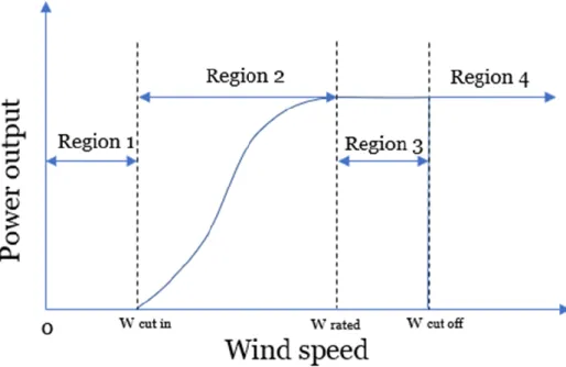
In “Handbook for wind energy engineering” from (2017), Letcher explains the characteristic power curve for a pitch regulated turbine. Letcher defines the minimum speed for which electricity can be generated as cut-in speed. All wind speeds below a threshold, which is typically around 4 m/s, does not generate enough rotational power to kick-start the turbine. This is illustrated in Region 1 in Figure 1. Region 2 in Figure 1 shows how the power
generated is increasing with higher wind speeds which is then regulated in Region 3 when the rated power is obtained. The rated power is defined by the maximum rotational speed limit for which the rotor is allowed to run. This speed limit is often set by the manufacturer to increase the longevity of the blades by preventing and minimizing bird impacts, rain and erosion according to Letcher. At the cut-off wind speed at typically 25 m/s, which is also the maximum wind speed, the rotor is brought to a standstill by a break to prevent structural damages. The wind speeds over 25 m/s generate power but are regulated to not exceed the 25m/s threshold for safety reasons by pitching the blades.
Figure 1 - A characteristic power curve for a pitch regulated wind turbine, Inspired by Sohoni et al. (2016).
Power curves are an easy way to illustrate the relationship between the output power and wind speed. A typical power curve for a pitch regulated wind turbine has a cut-in speed and a cut-out speed. In Figure 1, inspired by Sohoni et al. (2016), a power curve is shown, which is typical for a pitch regulated wind turbine.
8
Issues with Power Curve Modelling
Many attempts have been made to identify periods of nominal and fault operations of wind turbines with the help of power curves, and some have further tried to calculate production losses and tried to identify them. The methods vary a lot, but the most used way is to look at power curves. Power curves can be helpful when checking the performance of a turbine. It can be used for forecasting production or, if data is at hand, to calculate power losses. As earlier mentioned, different assumptions are made when trying to identify icing, and there is no standardization, which makes the results very variant. A few minor deviations in
assumptions and limitations can cause considerable alterations in the final result, causing disparity site-wise giving questionable results.
In 2016 Vaishali Sohoni, S.C. Gupta and R. K. Nema wrote in their critical review on
modeling wind turbine power curves that there are several essential issues to consider while modeling a power curve. They stated five main issues; Difference in turbine models, Cut-in and Cut-off behavior, Single versus a group of turbines, Influencing factors, and International Electrotechnical Commission (IEC) 61400-12-1 Standard. Four issues being of enough
relevance to get a further explanation in the titles that follow.
3.2.1.1. Difference in turbine models & Cut-in/Cut-off
Power curves will differ depending on manufacturers and models. The characteristics will then be different depending on the cut-in and cut-off behavior of the turbine. There are two main ways of handling turbines near cut-in and cut-off wind speeds; Pitch regulation and stall regulation. Stall regulated turbines have solid rotor blades, whereas pitch-regulated wind turbines which are dominating the market today can pitch the rotor blades.
The cut-off and cut-in fluctuation behavior that occurs between shut down and restart of the turbine affects the productivity of the turbine. The effect has on the productivity change depending on wind patterns and terrains referred to as hysteresis in the literature, where turbulent winds require more frequent starting and stopping.
3.2.1.2. Single turbine versus Wind farm
A prediction of the power output is always given by the manufacturer; this prediction is presented in a power curve for the specific turbine type at hand. Wind energy production is highly affected by the stochastic nature of the wind. In a wind farm, one turbine can have a different power output from a nearby turbine of the same turbine model. This can be caused by shadowing effects, also called wakes. A single wind turbine causes the downstream wind (the wind behind the plant), which disturbs the upstream wind flow for a nearby plant. The difference can also lay in wear/tear, aging, dirt, or ice deposition on blades. Sohoni et al. stress the importance of considering this while modeling big wind power farms.
9
3.2.1.3. Correlation factors
Correlation factors or influencing factors, as one might call them, are factors that cause the power curve to depart from the theoretical value. By taking various site-specific factors into account, it can be easier to understand the resulting power curve. The wind is the prime factor that affects the power output, and therefore the power curve. Trees, buildings, and other topologies at site influence the direction and velocity of wind streams. Blade geometry, which is disturbed when there is ice build-up on blades, leaves the aerodynamics of the blade alteration, which causes power output deterioration.
Air density is changed due to pressure, temperature, and humidity on site. And is directly correlated to ice accretion and, therefore, power production. By normalizing data from air density just like St. Martin et al.,(2016) did in their report, it is much more likely that outliers from other influencing parameters will be found and that the power production losses are better reflecting the reality. The vibration of the nacelle and tower is also a factor caused by ice accretion. In 2016, Skrimpas et al., a study where they detected ice build-up by utilizing a power curve and nacelle vibration data.
Temperature is a critical factor for ice accretion; water freezes as the temperature go below 0 degrees Celsius. Depending on the temperature, different types of ice formations are created. There are typically two types of icing conditions stalked about in the wind industry:
metrological icing and instrumental icing. Metrological icing occurs when the metrological conditions for ice accretion are favorable. Rime ice forms at temperature from 0° C down to -40° C. Glaze ice, however, is usually formed at a combination of high speeds, high
temperatures (between 0° C and -6° C), and high liquid water content (Yirtici et al., 2019). Instrumental icing is periods when ice remains at a structure and/or an instrument. Logically, ice does not disappear at the same time as the temperature goes above 0° C.
10
SCADA data
What Sohoni et al. fails to mention it their report from 2016, is the fact that wind speed measurements on a turbine are made by an anemometer that is placed in the back of the rotor. This means that the anemometer is placed in the wake of the rotor leading to big uncertainties regarding the actual wind velocities. Laakso et al., (2010) claim in their study that the wind speed underestimations can be as high as 30%. Manufacturers are using a correction factor in SCADA to improve the accuracy of the data, yet there is still a big uncertainty with the measurements.
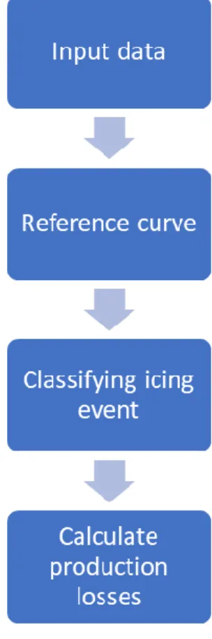
In the studies where SCADA data have been available, the structure for identifying icing losses follows the same structure which is illustrated in Figure 2. The input data or the SCADA is used to make a reference power curve that should reflect the ideal power production of a turbine and/or an entire site. A reference power curve is a curve for the optimal performance of a turbine or can be made to represent an entire wind farm. SCADA provides alarm codes which are normally indicating that the turbine is operating in normal condition versus when it is not. A classification of when icing is supposedly happening is done and the data is then filtered based on classifications of icing events. The production losses are then calculated by identifying the ice-losses which is done by comparing the reference curve with the data points classified as icing events.
11
Methodology Approaches
Hansson et al. (2016) wrote a report on quantification of icing losses in wind farms as a part of Energiforsk’s research program Vindforsk IV which was carried out by Kjeller Vindteknikk. In the report, three main ways of defining ice-losses were found and further explained. The first method presented; estimated ice losses based on a comparison between summer and winter power curves. Turbulence, atmospheric stability, and air density may be substantially different during winter as compared to summer which is an issue that Energiforsk highlight in their report. This would inadequately represent the expected power during winter with the power curve estimated based on summer data.
The second method, based on analyzing the variations around the power curve and assuming these variations will equal out if analyzed over a long enough time. Possible deviations from this would then be caused by icing. Energiforsk means that this method can give reasonable estimations of icing long-term but when shorter periods are investigated the method fails to estimate icing losses.
Lastly, a method of putting a threshold value on the power curve and identify periods when the power production comes below these threshold values as periods with icing is presented. The power tends to fluctuate around a given power curve depending on other parameters such as wind direction, atmospheric stability, and turbulence. Energiforsk points out that the method might not be able to find all the cases for which icing losses occur, but might, on the other hand, identify periods that can be associated with icing although icing is not the problem.
Classification of icing losses
Research by Aziz et al. (2019) amongst others (Byrkjedal et al., 2015; Davis et al., 2015; Hansson et al., 2016; Sohoni et al., 2016) have used SCADA data to create prediction models and/or models for measuring icing losses. SCADA covers all the data needed to perform power curves. Depending on the data needed at hand, a dataset from SCADA can cover millions of data points which makes it a powerful source of knowledge. There are however different assumptions made while making power curves. Byrkjedal et al., use the same method as Davis et al., where SCADA data is used to calculate the power curve by taking the median power values from wind speeds binned with 0.5 m/s intervals, an IEC standard according to Sohoni et al. (2016).
12
In the report by Byrkjedal et al. from 2015, an operational forecasting model for icing is developed for four wind farms located in Sweden. Data from 12 Swedish metrological stations are used to develop the model. The reference data that is used for the model calculates the power curve by using SCADA data. The report is therefore interesting to look at since the reference data use the median power output values from all wind power sites, and divide, or bin, them into 0.5 m/s intervals. Data for periods with curtailed power output is removed, they are also looking at alarm codes. An alarm code is removed along with the data from the pro- and preceding 10-minute time steps. The data is further analyzed by filtering all data points which have a temperature below 3 °C if these fall below the 10th percentile threshold of the median power for more than 3 consecutive time steps or 30-minutes they are classified as icing. Even though the main purpose of the study was to forecast icing, the resulting ice-losses identified from the SCADA data are highly interesting to look at. The ice-ice-losses for the sites were observed to be 22%, 9%, 10%, and 13% respectively for each site. Justification as to why the results diverge is yet to be given.
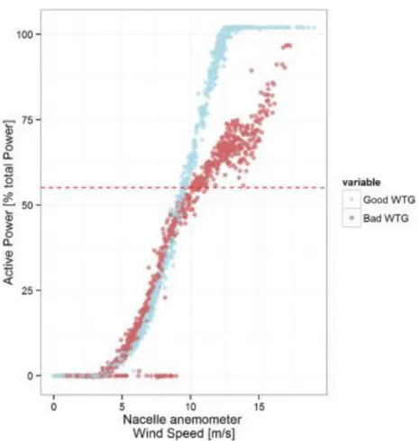
Figure 3 - Normal vs abnormal power curve. Retrieved from: Papatheou et al. (2017).
The approach for data cleaning made by Byrkjedal et al. (2015b) was to first remove data points when the turbine was identified to be in a derated state. Thereafter, data points with error codes that could not be linked to icing were removed. The data point before and after the error code was also removed since the error flags were only given to the classic 10-minute interval given by SCADA. The only indications for icing were therefore the data points
13
uncertainty with this method is that there is no way to know exactly when the error occurred due to the 10-minute time step of the SCADA data.
In a report by Davis et al. (2015) four wind parks with known icing occurrences were investigated and compared with each other. Three different methods were used to observe indirect ice detection using a power curve deviation. Davis et al. (2015) concluded that setting an ice threshold of the 10th percentile of the observed power curve data during normal
operation with a 2-h minimum duration was the best approach for identifying ice-losses. The reference power curve was based on 40 % of the total percentile to fit the local regressions since the raw data made the percentile curves quite ragged due to outliers. The suggestion is to base the percentile on data for at least one year. Further, a smoothing function was
suggested to be applied to the percentile to remove outliers which would be caused by limited numbers of data points. A positive 2.5° C bias in the nacelle temperature was also found in one of the two turbines that were studied. They also investigated different scenarios where the temperature threshold for iced data was set from -2° C to +4° C.
Homola et al. wrote a report in 2009 about energy production losses due to iced blades and instruments for three wind power sites in Norway and Sweden. They use power curves to identify ice losses with both 10-minute and 1-hour historical data, it is however not specified if the data is SCADA data. Since the expected power curve is based on data of the median power production between the 1st of May to 1st of October where data points with an ambient temperature above +2° C were used, it is safe to imply that the data in hand is indeed given by SCADA. They divide the wind speeds into 0.5 m/s bins, just as (Byrkjedal et al., 2015; Davis et al., 2015). Wind speeds lower than 5 m/s were filtered out due to the nonlinearities associated with starting and stopping the turbine. An 85% threshold was set to identify low power production due to ice. The difference between the expected power from the power curve and the actual power was counted as a power loss.
In comparison to the other studies mentioned, Homola et al. (2009) use a reference power curve that uses both non-iced data and iced data. The method is, therefore, underestimating the power losses since the power curve is based on all data to generate the power curve. Some problems with overproduction which were linked to the anemometers were also identified. The anemometers were giving a too low value which thereby gave an unrealistic good power production. However, the calculated losses were only 0.5 percent for this site with Siemens turbines which in contrast to the other two sites is very low, mainly due to the faulty values from the anemometer. The threshold was therefore modified to 115 percent of expected power plus 50kW for velocities over 3 m/s. The second site had a production loss of 5 percent whereas the third site had more than four times higher production losses during winter compared to summer, both being Vestas turbines. For the third turbine that means that the average production losses where 27.9% during winter compared to 6.6% during summertime.
14
Task 19
Though it might seem like there is no standardized way of detecting ice-losses, IEA founded a task group in 2002 called: Task group 19 – a division in IEA founded to gather and provide information about wind energy in cold climates. In 2019, Task 19 published a method for determining production losses. The method, called task 19 IceLoss method (2019), use SCADA data to calculate icing losses and is publicly available as a Python code released on GitHub in 2019. The method is acknowledged by the industry, yet due to its recently being published, there are no studies made to validate the method.
The method complies with Energiforsk’s findings of three types of methods. However, Task 19 IceLoss method combines the three methods mentioned by Energiforsk in a new way which deals with the main issues also stated by Energiforsk. Task 19 further affirm a warning about nacelle temperatures which in some cases have shown a constant bias of +2 to 3°C due to radiation heat of the nacelle. Task 19 also states that ice build-up deteriorates the power output or results in overproduction due to iced anemometers.
3.3.2.1. Reference Power Curve
The structure of the method is based on percentiles of the reference power curve which is created by non-iced data classified by data points above an ambient temperature of 3° C. Air density is corrected to hub height and since air pressure is normally not given by SCADA data, static pressure is calculated based on on-site elevation above sea level. Site air density and pressure are then used to calibrate nacelle wind speeds as follows:
Equation 1 𝑤𝑠𝑖𝑡𝑒= 𝑤𝑠𝑡𝑑∗ (𝜌𝑠𝑡𝑑 𝜌𝑠𝑖𝑡𝑒) 1 3 = 𝑤𝑠𝑡𝑑∗ ( 𝑃𝑠𝑡𝑑 𝑇𝑠𝑡𝑑 𝑃𝑠𝑖𝑡𝑒 𝑇𝑠𝑖𝑡𝑒 ) 1 3 Equation 2 𝑤𝑠𝑖𝑡𝑒= 𝑤𝑠𝑡𝑑∗ (𝑇𝑠𝑡𝑑 𝑇𝑠𝑖𝑡𝑒(1 − 2.25577 ∗ 10−5∗ ℎ)5.25588) 1 3
Table 1 – Explanatory nomenclature table for Equation 1 and Equation 2
wsite Calibrated nacelle speed
wstd Measured nacelle wind speed
Tsite Nacelle ambient temperature (K)
Tstd 15°C (288.15 K) ambient temperature
Psite Air pressure at site
Pstd 101325 Pa ambient air pressure
h Site elevation in meters above sea level
𝝆𝒔𝒕𝒅 Calculated density at site
15
To make the power curve calculations, the data is binned with the same range as the wind speeds. Only bins with at least 6 hours of data are used to get a representative result. Several calculations are made for the bins:
• Median output • Standard deviation • 10th percentile
• 90th percentile
• Power curve uncertainty i.e. standard deviation divided by power • Sample count in the bin
3.3.2.2. Icing Events
Icing events are divided into three different classes by Task 19; a) decrease in production, b) standstill, c) overproduction due to the iced anemometer. Icing event class a) is started if the temperature is below 0°C, and power is below the 10th percentile of the reference power curve for 30-minutes or more. It ends if power is above the 10th percentile for 30 minutes or more. For each 10-minute data point, it is decided whether that data point is classified as affected by ice or not. If the data point is classified as an iced-data point, and if nearby data points are also ice affected so that the data points create a 30-minute consecutive trace of ice-related data, then the data points are ice-losses.
Icing event class c) is started if the temperature is below 0°C AND power is above the 90th percentile of the reference power curve for 30-minutes or more. It ends if power is below the 90th percentile for 30 minutes or more. While icing event b) follows the same idea as icing event a) with a 10th percentile curve, the difference is that the icing event starts when the power is below 10th percentile AND results in a shutdown for at least 20 minutes. It ends if the turbine is started AND the power is above the 10th percentile for 30 minutes or more.
3.3.2.3. Production losses due to icing
Once the icing events have been identified the production losses can be calculated. The difference between the reference and actual measured output power for each time step is calculated.
16
Kjeller Method
Kjeller Vindteknikk is a consultancy company within the wind power and wind engineering industry in the Nordics. In their report, Hansson et al. (2016), together with Energiforsk, investigate six different methods, which are being analyzed. These methods can be divided into two different groups, where the first group is depending on one or more ice-free turbines on a wind power farm to be used as references. The other group which is preferred by
Hansson et al. (2016), is based on wind and production data.
In the same report, a methodology for the post-construction of estimating production losses due to icing is presented. By adjusting varying densities according to IEC 61400-12-1 a taking the median wind speed bins at very 0.5 m/s just as others have (Byrkjedal et al., 2015; Davis et al., 2015; Homola et al., 2009; Task19, 2019) and filtering out the following data:
• Data with alarm codes and the time step after the alarm occurred.
• Data for periods with curtailed power output (i.e., periods when the wind turbine is operating in a lower capacity than it should).
• Data that may be affected by icing, temperatures below 3°C.
• Occasions when nacelle wind speed is more than two meters above cut-in, and the power production is less than 5 kW.
A reference power curve is then constructed by making a 10-percentile power curve for each turbine and not site-wise like Task19 (2019). This does also mean that Kjeller Vindteknikk did not take the overproduction due to iced anemometers into account is this paper, in contrast to Task 19, where a 9o-percentile power curve is also used. Hansson et al., (2016), emphasize the need for a long-term reference dataset since there is a considerable variation in power output from one year to another. Furthermore, it is assumed that there is less icing on turbines at locations with low elevation and that it is more icing on turbines at high elevation locations, which are then validated in the report. Another distinctive difference is that Kjeller Vindteknikk filter away the nacelle wind speeds around the cut-in. Since the cut in is normally 4 m/s, all the data points with wind speeds below 6 m/s are not being
accounted for by Kjeller in the reference curve.
The ice-losses are, however, defined almost identically to Task19 (2019). The 10th percentile is used as a reference. All data points which are below this reference, have a temperature below 3° C, have a turbine which indicates normal operation, and that this happens three time steps in a row, are classified as ice losses.
17
De-icing systems
De-icing systems are a fairly new phenomenon in the wind power industry, and it was not until 2004 when the first de-icing systems were installed by Enercon (The Ice Issue - The Ice Issue | Winterwind | Where Theory Meets Practice, n.d.). De-icing systems depend greatly on measurements. Placed at the top of the wind turbine tower, the hub is located. Here, sensors are placed to check numerous weather data to operate the wind power plant and to maximize power production safely. When icing occurs, these sensors can be shut down or be unable to gather accurate information. This can cause misdirection of the rotor or that the steering of the plant stops operating event though the wind is within the legal speed limits (4-25m/s). Fakorede et al. (2016) wrote a comparison between ice protection systems where they concluded that improving the cold-climate performance of wind turbines has become a “sine qua non” condition, meaning it is a necessary action for the continued development of the wind power industry. While they state numerous de-icing systems, there are two that this literature study will focus on: Blade heating and OWI.
Blade heating
When discussing blade heating, there are generally two types of systems that are intended: Heated air and Electrically heated mats. These systems are implemented in the rotor blades. For Electrically heated mats, the system consists of heating coils or carbon fibers that are placed strategically on the blades, either inside the membrane or laminated on the surface of the blades. The coils are then heated by electricity taken from the grid at standstill; shown as negative power production in the SCADA data. The heated air technology is also used at a standstill; the concept is to inject warm air into the blades and warm the ice by heat flux. This system is used both for de-icing purposes but also for anti-icing, which prevent ice accretion. Normally, one of these two systems are used but there are also examples when they have been used together. Wallenius & Lehtomäki (2016) write in their overview on cold climate wind energy challenges, that a combination of surface heating and hot air heating could lead to better coverage of ice protection in terms of efficiency over a wider area of ambient conditions.
For the blade heating to be turned on the sensors need to detect icing, normally, this is done by checking the reference power curve with the actual power production and the ambient temperature. If the sensors are detecting high wind, low temperature, and low power
production (or in some cases: no production) the turbine is shut down. It is when the rotor is completely still that the heating is put on for a certain amount of time, then the ice is
estimated to have time to slide off and the rotor is yet put in motion. If the power production is still low, the system is required to stop once again for another de-icing cycle. This
procedure will continue until a production within proximity of the reference power curve is reached.
18
One reason for not operating with blade heating would be the risk for ice-throw. Ice from the rotor blades can be thrown 90 meters at a very high speed, which can cause a severe health and safety risk for the surrounding environment (Davis et al., 2015). The main reason for not running any kind of blade heating while running the turbine is however another. In 2011, Oliver Parent and Adrian Ilinca wrote a critical review on anti-icing and de-icing techniques for wind turbines. The reason that cooling of the blade from the slipstream would be so high that it would require extreme amounts of energy from the grid to heat the blade which would not make it beneficial to run the heating system
Blade heating can be both expensive and very power consuming. Since the blade heating requires the plant to stop the turbine, the possibility to produce power with slight
ice-formation is completely removed, which means that we have a power loss higher than due to the actual icing. Yet, removing the ice makes further ice formation impossible, and the turbine will be able to operate without standing still.
OWI – Operation with Ice
OWI is a software for active pitch control. The system is not an ice protection technique, as Ville Lehtomäki mentions in his report for IEA in 2016, it is used for pitching the rotor blades in the optimal direction of the wind to keep the turbine operating throughout an icing event. When ice is formatted on rotor blades, the angle of attack is changed. What the OWI then does is that it uses the pitch system to find the optimal angle for maximum power
production. It does not require additional power consumption and is easily installed in already erected pitch-regulated turbines.
Lehtomäki (2016) also mention that pitch systems can suffer when exposed to cold weather; insufficient lubrication of components can damage gears. When a turbine can no longer operate the pitch system, it will either have to wait until the ice melts, or it must rely on a blade heating system. Y. Zhang et al. (2020), therefore, propose a combination of electric heating and active pitch regulation to have a rapid and efficient de-icing.
19
Summary literature review
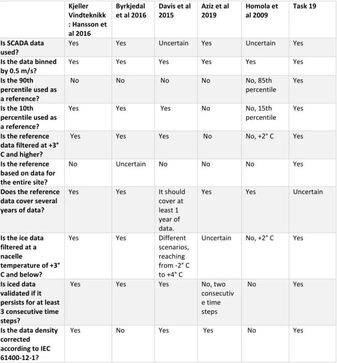
In Table 2, an overview is given for the different methodology approaches made by the earlier studies mentioned. Here, the most significant assumptions for this thesis are summarized.
Table 2 - Methodology assumptions
Kjeller Vindteknikk : Hansson et al 2016 Byrkjedal et al 2016 Davis et al 2015 Aziz et al 2019 Homola et al 2009 Task 19 Is SCADA data used?
Yes Yes Uncertain Yes Uncertain Yes
Is the data binned by 0.5 m/s?
Yes Yes Yes Yes Yes Yes
Is the 90th percentile used as a reference? No No No No No, 85th percentile Yes Is the 10th percentile used as a reference?
Yes Yes Yes No No, 15th
percentile
Yes
Is the reference data filtered at +3° C and higher?
Yes Yes Yes No No, +2° C Yes
Is the reference based on data for the entire site?
No Uncertain No No No Yes
Does the reference data cover several years of data?
Yes Yes It should
cover at least 1 year of data.
Yes Yes Uncertain
Is the ice data filtered at a nacelle
temperature of +3° C and below?
Yes Yes Different
scenarios, reaching from -2° C to +4° C
Uncertain No, +2° C Yes
Is iced data validated if it persists for at least 3 consecutive time steps?
Yes
Yes Yes No, two
consecutiv e time steps
No Yes
Is the data density corrected
according to IEC 61400-12-1?
20
4
PROPOSED ICE DETERMINING METHOD
The assumptions made in the formation of this method hold its ground in the approaches made by the studies in the literature study. A combination of threshold power curve based on turbine operational status and measured temperature criterion was used to create the ice determining code. The code from which ice loss data will be extracted is made in R-studio with the datasets given by an SGRE server. Firstly, the code is downloading data by choosing the site, tower height, alarm codes, and the dates from the year to be analyzed. It is after the data-download that the data is processed.
From the literature study, it is concluded that the power curve should be based on the use of polynomial values to look at the linear regression. Further, the maximum theoretical power production is defined as the production of the turbine as if it was to operate with blades free from ice. The ice losses are calculated based on data for one site at a time. To ensure ice-free data, the reference power output data is based on data between the warmest months for Sweden, i.e., May throughout September. What alarm codes for which the central part of the filtrations was done on, is based on the combination of two recommendations made by other internal reports from SGRE, which has tried to make similar identifications of ice losses from SCADA data. Before any filtration is done on the raw data, NAN values are removed. Also, for both reference and ice datasets, the density is corrected by using the same calculation as Task19 (2019), stated in Equation 2 found in the literature study.
Site information
Two sites are initially investigated; they will be called Site 1 and Site 2. They are both located in the middle of Sweden. However, Site 2 is located higher up in the country compared to Site 1. Site 1 has 26 turbines installed with a tower height of 122.5m, whereas Site 2 has 48
turbines installed with a tower height of 115m. The turbines for both sites are of model SWT-113 from Siemens.
Site 1 has blade heating installed with electric heating mats on all turbines from the initial installation of the turbines. OWI was installed at Site 1 in the middle of December 2015 on 13 of the 26 turbines at the site. It was not until late November in 2017 that the remaining turbines were installed with OWI. A test was made on the site in the winter between 2017-2018, to investigate the performance of OWI, turbines with equal power production were identified and divided into pairs of two. These twin-turbines were then evaluated by running OWI on just one of them to compare the power production between an OWI turbine and a non-OWI turbine. Site 2 operates with OWI on all turbines; the installation of OWI was done in December 2016.
21
Reference Curve
The methods in the literature study suggest that a reference dataset should be used to form a reference curve. Therefore, a reference dataset is made where the 90th and the 10th percentile is used as threshold to identify iced affected data points. Percentiles are a robust metric and can be used to capture the variance of a variable, according to Davis et al. (2015). The 90th percentile is extracted to see if data points that are affected by an iced anemometer can be identified, yet these data points are not counted as ice losses. The curve itself, is based on data from four different years, site-wise, to eliminate fluctuations caused by elevation of different sites, precipitation and to ensure that the data is ice-free. The gradient and constant for each bin are used as a reference for the upper and lower threshold to identify the data points which are affected by ice.
From the literature study, it was unclear what kind of data was preferred to use for a reliable reference curve. While Hansson et al. (2016) use data for one turbine as reference and Task19 (2019) use data for an entire site, the amount of historical data that the reference is supposed to use is rather unclear, yet most of the literature suggests data from at least one year. In this thesis, the reference curve is based on 4 different years: 2016, 2017, 2018, and 2019. These years were chosen to smooth out the variation in power output from one year to another, which is emphasized by Hansson et al., (2016) in the literature study.
Data pre-processing
The data pre-processing is a crucial stage since filtering out data open the possibility that iced or non-iced data has been filtered out wrongly. The reference data is therefore filtered with five different filters to out rule iced data:
• Filter1: Filters out all data points that are below 3 degrees Celsius. • Filter2: Filter based on data that have sufficient wind for production.
• Filter3: Filter away all data points which have a power output of 0 kW or below.
• Filter4: Filters out all alarm codes that have a power limit, which is not based on the nominal operation.
22
Threshold calculations
In the linear equation, found in Equation 3 below, k is the gradient, and m is the constant for the slope of the line. Linear interpolation is used by both Task19 (2019) and Hansson et al. (2016). Both the gradient and the constant are calculated for the upper 90th percentile and the lower 10th percentile by binding the data into intervals of 0.5 m/s. The length between the minimum and the maximum velocity is therefore split by 0.5 to get the optimal number of bins. The gradient for each bin is then calculated with Equation 4, where y represents the measured power from the dataset, and x is the velocity given in the dataset. The m-constant could then easily be extracted with Equation 5.
Equation 3 𝑦 = 𝑘 ∗ 𝑥 + 𝑚 Equation 4 𝑘 = 𝑦[𝑖+1,1]− 𝑦[𝑖,1] 𝑥[𝑖+1,1]− 𝑥[𝑖+1,1] Equation 5 𝑚 = 𝑦 − 𝑘 ∗ 𝑥
Defining ice losses
Scenarios
A difference in temperature between the tip of the blade and nacelle is not uncommon. The distance from the tip of the rotor to nacelle is 56,5m for both Scenarios in this study; it is a parameter that needs to be taken into consideration. The temperature threshold used for the significant part (Byrkjedal et al., 2015; Hansson et al., 2016; Task19, 2019) of the studies in the literature study, is set to 3° C. However, there is no clear explanation to why this would be the optimal temperature.
Three scenarios are therefore analyzed to see how much-iced data is discovered when the temperature filter is changed from a temperature of 0 to 3 and 5 degrees Celsius. The scenarios are a type of sensitivity analysis but are referred to as “scenarios” to make it more distinguishable from the sensitivity analysis explained in the title further down, which is not as extensive as the scenarios.
23
Data pre-processing
The dataset will cover at least 6x24x365 data points since the data is in a 10min resolution. Which equals to 52 560 data points for each turbine. As mentioned earlier, the data needs to be downloaded. To get the relevant data, 46 different variables where downloaded, leaving each site-dataset to be at least a 46x 52 560*turbines matrix. To minimize the number of data points, the dataset is filtered early in the code. Instead of filtering out the data points which can be connected to ice, which is done in the reference curve, these are the points that should be highlighted and saved in the new, minimized, dataset.
• Filter 1: Filter the operational status of the turbine and takes away the turbine stoppage not related to icing. Such as the untwisting of cables or wind speeds that are too high.
• Filter 2: Filters out all alarm codes that have a power limit which is not based on the nominal operation.
• Filter 3: Filter based on data that have sufficient wind for production.
• Filter 4: Filters out all alarm codes about actual turbine status which cannot be related to icing.
When downloading the data, the variables must be chosen beforehand. Date, time, velocity, power output, temperature, and alarm code are therefore extracted. The alarm codes are many and are divided into different categories. The categories concerned are stated below:
Description of alarm category Filtered on
Turbine operational state Stops which can be caused by icing Source of active power limit Limits defined by Nominal and
Converter power
Newest turbine alarm code Icing events and normal production. Actual turbine status Sufficient wind for production
These alarms have multiple codes for various occasions, and one year of data can have hundreds of different codes. To make the process of finding the relevant alarm codes more efficient the data is filtered based on codes that are only connected to icing events and normal production by looking at the newest turbine alarm code.
Calculating ice losses
Data points found below the 10th percentile threshold that also have a temperature below 0 degrees for Scenario 1, 3 for Scenario 2 or below 5 degrees for Scenario 3, and have a turbine that is operating normally is not enough to count as a data point affected by ice. If the
mentioned requirements are met and they are found for no less than 3 consecutive time steps, that is when the data point is defined as affected by ice.
24
In the code, the reference gradient and the slope constant are together with the measured velocity used to calculate the expected power output for every data point in every bin. In this part of the code, all NAN values are removed so that every single data point that has gone through the data pre-processing and is checked against the calculated expected power value. This is a very time-consuming step in the code and the most important part. The measured data point which is then highlighted as smaller than the calculated expected power, is then saved as data affected by ice.
The icing events are then found and can be extracted. The ice losses are calculated by using the difference between the expected power and the actual measured power. Since the data is given as kW for 10 minutes, the data was converted to kWh by dividing the power output with 6. Thereafter the code summarized the data for each turbine and year. Further processing of the data was made in Excel to convert the annual ice losses to both MWh and in percentage for an entire site.
25
Correlation factors
Since temperature and precipitation have a big impact on ice build-up, it is interesting to see whether any correlation can be found between the annual ice losses, temperature, and precipitation. January, February, and December are what SMHI defines as winter months, which is why the average temperatures and precipitation given in the tables below are based on the monthly average precipitation for these months. The SMHI data was given by the metrological station closest to the site location and were extracted from SMHI – Swedish Meteorological and Hydrological Institute (2020). Only data for the investigated years were extracted.
Table 3 - Average winter temperature and precipitation Site 1.
Year Monthly (Dec/Jan/ Feb) average temperature [°C]
Monthly (Dec/Jan/ Feb) average precipitation [mm]
2016 -7.93 23.07
2017 -7.30 27.13
2018 -9.37 43.80
2019 -6.10 30.77
Table 4 - Average winter temperature and precipitation Site 2.
Year Monthly (Dec/Jan/ Feb) average temperature [°C]
Monthly (Dec/Jan/ Feb) average precipitation [mm]
2016 -7.77 39.13
2017 -5.93 44.20
2018 -8.53 39.50
2019 -6.77 34.77
The reason for this data being extracted from SMHI is that precipitation is not something that can be found in SCADA. Precipitation measurements are made by additional software that is not connected to SCADA, and since the data is not measured in the same time
resolution as SCADA it was not investigated whether it could be possible to merge these two data sets.
26
Sensitivity Analysis
To validate the assumptions made for the ice loss determining method, a sensitivity analysis has been performed.
Reference curve
A sensitivity analysis is made for the power reference curve. The raw data for the power reference curve was changed from May-Sep to Jan-Dec, and June-July to see how much-iced data could be explained by adding more/fewer data points. Hence it was only analyzed for 2019 on Site 1 on Scenario 2, where the temperature threshold was set to 3° C.
Temperature threshold
A minor sensitivity analysis was also made on the temperature thresholds beyond the ones in Scenario 1, 2, and 3. In this analysis, a threshold was set to 1.5 and 6 degrees respectively to see how much more/fewer ice losses that could be found. It was however conducted for data from the year of 2019 on Site 1, with a reference curve based on data from May to September (the same reference curve as for the scenarios).
27
5
RESULTS
The ice losses found in Table 5, Table 8 and Table 9 will be presented with a manipulation-factor to normalize the values. Therefore, the actual ice losses, which are first calculated in percentage of the expected power output, is divided with a number. This number will be unknown to the reader yet known by the author of this report and SGRE. The normalized ice losses are then multiplied with 100. This normalization is further explained by Equation 6. Both sites are divided by the same number so that it is possible to show a ratio between the two different sites.
Equation 6
𝑁𝑜𝑟𝑚𝑎𝑙𝑖𝑧𝑒𝑑 𝑖𝑐𝑒 𝑙𝑜𝑠𝑠𝑒𝑠 =𝐴𝑐𝑡𝑢𝑎𝑙 𝑎𝑛𝑛𝑢𝑎𝑙 𝑖𝑐𝑒 𝑙𝑜𝑠𝑠𝑒𝑠
𝑚𝑓𝑎𝑐𝑡𝑜𝑟 ∗ 100
This is done to avoid exploiting confidential data from the owner of the wind farms.
Additionally, it is important to highlight the fact that the power curves in the sections below have thousands of data points. And that what may seem like one data point might have hundreds or thousands more that are on top of each other, or very close to one another.
Reference curve
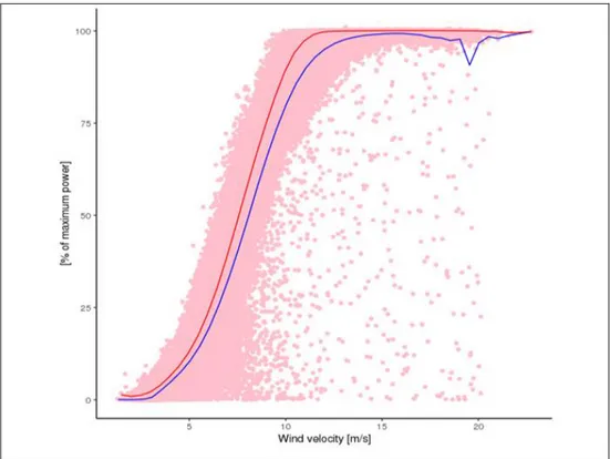
In Figure 4 and Figure 5, the reference power curves for the two sites are presented. These reference curves are used in Scenario 1, 2, and 3. The reference curves are based on data between May-Sep in the years of 2016-2019. The blue line represents the 10th percentile while the 90th percentile is represented by the red line. The pink points in the actual power curves below represent the reference curve data. A distinctive dip can be seen in the 10th percentile line for Site 2. Both reference curves have a 10th percentile and a 90th percentile line which seamlessly merge at the highest bins. The reference curve for Site 1 has undeniably several data points near a zero power production at higher wind speeds above 10 m/s than the reference curve for Site 2 shows.
28
Figure 4 - Reference curve for Site 1. The y-axis is showing the percentage of the maximum nominal power and the x-axis showing the wind velocity in m/s.
Figure 5 - Reference curve for Site 2. The y-axis is showing the percentage of the maximum nominal power and the x-axis showing the wind velocity in m/s.
29
Actual power curve
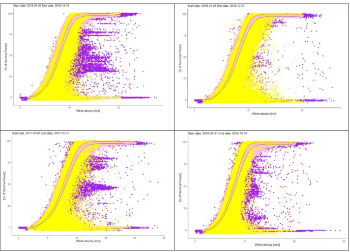
The colored diagrams that are featured in the sections below are the actual power curves of the sites, presenting the turbine power data and the nacelle wind speeds. The blue line represents the 10th percentile, while the 90th percentile is represented by the red line. The pink points in the actual power curves below represent the reference curve data. The purple points are the raw data for the specific year, whereas the yellow points are the data points that are affected by ice. The points below the 10th percentile is therefore defined as ice losses while the yellow points above the 90th percentile are the data points that are affected by an iced anemometer.
Scenario 1
In Scenario 1, a temperature threshold of 0° C is set to identify ice losses. As can be seen in Figure 6 and Figure 7, the actual power curves are departing from the reference curves. Site 1 is diverging more distinctively than Site 2. In Figure 6, the power curves for 2016, 2017, and 2019 show a clear deviation from the reference curve. This type of deviation can also be detected in 2016 for Site 2, although not as definite as for Site 1. The ice losses for 2018 in Figure 6 are more concentrated near a zero power output.
Figure 6 - Actual power curve for Site 1. Scenario 1. From the upper left corner to the right are the years: 2019 and 2018. To the lower-left corner to the right are the years: 2017 and 2016.
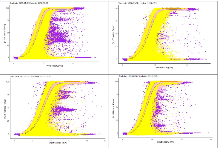
30
Figure 7 - Actual power curve for Site 2. Scenario 1. From the upper left corner to the right are the years: 2019 and 2018. To the lower-left corner to the right are the years: 2017 and 2016.
Scenario 2
Scenario 2 uses a temperature threshold of 3° C to identify ice losses. In Table 5, the ice losses for the turbines for Site 1, which underwent the test between December 2017 and February 2018, are presented. As can be seen, the ice losses where in general higher in 2018 than in 2017, but the difference between the turbines installed with OWI and the turbines without is much bigger for 2018 than for 2017.
Table 5 - Annual ice losses Site 1, Scenario 2, turbines with OWI vs. turbines with no OWI.
Average ice loss with manipulation factor- 2018
Average ice loss with manipulation factor - 2017 Turbines with OWI 155% 120% Turbines without OWI 182% 119%