Västerås, Sweden
Thesis for the Degree of Master of Science in Engineering - Robotics
30.0 credits
VISION-BASED ROBOT CONTROLLER
FOR HUMAN-ROBOT INTERACTION
USING PREDICTIVE ALGORITHMS
Hannes Nitz Pettersson
hpn15004@student.mdh.se
Samuel Vikström
svm16001@student.mdh.seExaminer:
Ning Xiong
MDH, VästeråsSupervisor(s):
Carl Ahlberg
MDH, VästeråsMiguel LeónOrtiz
MDH, VästeråsCompany Supervisor(s):
Wicktor Löw
Nordic Electronic Partner, Västerås
Abstract
The demand for robots to work in environments together with humans is growing. This calls for new requirements on robots systems, such as the need to be perceived as responsive and accurate in human interactions. This thesis explores the possibility of using AI methods to predict the movement of a human and evaluating if that information can assist a robot with human interactions. The AI methods that were used is a Long Short Term Memory(LSTM) network and an artificial neural network(ANN). Both networks were trained on data from a motion capture dataset and on four different prediction times: 1/2, 1/4, 1/8 and a 1/16 second. The evaluation was performed directly on the dataset to determine the prediction error. The neural networks were also evaluated on a robotic arm in a simulated environment, to show if the prediction methods would be suitable for a real-life system. Both methods show promising results when comparing the prediction error. From the simulated system, it could be concluded that with the LSTM prediction the robotic arm would generally precede the actual position. The results indicate that the methods described in this thesis report could be used as a stepping stone for a human-robot interactive system.
Acknowledgement
We offer our thanks to our supervisors, Carl Ahlberg and Miguel LeónOrtiz for their excellent guidance in all aspects of the work.
We would also like to thank Wicktor Löw at NEP for his understanding and support during this thesis work. Gratitude is also extended to NEP for providing the opportunity and equipment to make this work possible.
The data used in this project was obtained from mocap.cs.cmu.edu. The database was created with funding from NSF EIA-0196217.
Abbreviations
AI Artificial Intelligence NEP Nordic Electronic Partner MDH Mälardalens Högskola MSE Mean Square Error LSTM Long Short-Term Memory ESN Echo State Network DC Direct Current SGM Semi-Global Matching RNN Recurrent Neural Network CNN Convolutional Neural Network ANN Artificial Neural Network
MTCNN Multi-Task cascaded Convolutional Neural Network DOF Degrees of Freedom
PID Proportional-Integral-Derivative PSO Particle Swarm Optimization EMF Electromotive Force
Contents
1 Introduction 1 2 Background 2 2.1 Neural networks . . . 2 2.2 Stereo vision . . . 3 2.3 DC motors modelling . . . 5 3 Problem Formulation 6 3.1 Hypothesis . . . 6 3.2 Research Question . . . 6 3.3 Limitations . . . 6 4 Related Work 7 4.1 ESN prediction . . . 7 4.2 LSTM prediction . . . 7 5 Methodology 9 5.1 Problem formulation . . . 9 5.2 Literature study . . . 9 5.3 Experiment design . . . 9 5.4 Development . . . 105.5 Test and debug . . . 10
5.6 Thesis conclusion . . . 10 6 Method 11 6.1 Face detection . . . 11 6.2 Depth . . . 11 6.3 Simulation . . . 11 6.4 Dataset . . . 11 6.5 Prediction algorithm . . . 12 6.5.1 Dropout layer . . . 12
6.6 Hyper parameter optimisation . . . 12
6.7 K-fold cross-validation . . . 13
7 Ethical and Societal Considerations 14 8 Experimental setup 15 8.1 Spatial face tracking . . . 15
8.1.1 Camera setup . . . 15
8.1.2 Face detection . . . 15
8.1.3 Trajectory alignment . . . 16
8.2 Data manipulation . . . 16
8.2.1 Motion capture . . . 16
8.2.2 Velocity and acceleration calculations . . . 17
8.2.3 Standardising the data . . . 17
8.3 Network architecture . . . 17
8.4 Hyper parameter optimisation . . . 17
8.5 prediction error evaluation . . . 18
8.6 Simulation . . . 18
8.6.1 Robotic model . . . 19
8.6.2 Joint model . . . 19
8.6.3 PID controller . . . 19
9 Results 21 9.1 Prediction network . . . 21 9.2 System integration . . . 24 9.3 Actuators . . . 28 10 Discussion 29 10.1 Prediction network . . . 29 10.2 System integration . . . 29 10.3 Actuators . . . 30 11 Conclusions 31
11.1 Research questions summary . . . 31 11.2 Future work . . . 32
References 34
List of Figures
1 A simple sketch over a single node in a neural network . . . 2
2 Architecture over a LSTM cell and with its gates annotated . . . 3
3 Architecture over a ESN with the different layers annotated . . . 3
4 The relation of points in world space to image planes of two cameras and the relation of the projected light path to the epipolar line in a second image plane. Where Cl is the left camera position and Cr is the right one . . . 4
5 Flowchart over engineering process that is followed in this thesis work . . . 9
6 Calculating the next velocity of a particle in PSO . . . 13
7 Demonstration of K-fold cross validation . . . 13
8 Intel RealSense D455 camera . . . 15
9 Physical camera setup . . . 16
10 Basic architecture over a LSTM network . . . 17
11 Robot model drawn for a random joint configuration. . . 19
12 Diagram of closed loop joint controller . . . 20
13 Graphs over a 3D trajectory from the validation set with the correlated prediction trajectory for 4 different prediction times. A is over a prediction trajectory where the Neural networks try to predict 1/2 of a second into the future, B is for 1/4 of a second, C is for 1/8 of a second and D is for 1/16 of a second. . . 22
14 Graphs over trajectory from the validation set split up into X, Y and Z axis. The neural networks is trying to predict 1/4 of a second in the future. . . 23
15 Graphs over trajectory from the validation set split up into X, Y and Z axis.The neural networks is trying to predict 1/16 of a second in the future. . . 23
16 Results of simulation based on LSTM prediction compared to simulation result for no prediction. A is for 1/2, B is for 1/4, C is for 1/8, and D is for 1/16 second. . . 25
17 A show the LSTM prediction result for 1/4 second with 6 Hz sampling. B show result for interpolated 30 Hz sampling rate. . . 26
18 Simulation result for a local region in the X axis input with all simulated prediction times. Subplot A contain LSTM results and B the ANN results . . . 27
19 Performance of actuator models for each prediction time plotted with zero mean and a standard deviation of one. Lines fitted using linear regression show the data trend as torque increases with motor index. . . 28
List of Tables
1 Optimised values for LSTM . . . 18
2 Optimised values for ANN . . . 18
3 DC motor parameters . . . 20
4 Error over different prediction methods . . . 21
5 Resulting error from simulation as Euclidean distance from target position. . . 24
6 Proportion of duration where prediction results in smaller error. . . 24
7 System error reduction from interpolated data. . . 24
8 LSTM and ANN performance gain from interpolated data. . . 24
1
Introduction
Ever since Karel Čapek introduced the term robot in the early 1920s, people have imagined human interaction as a core attribute of what a robot is. The industrial revolution brought with it the idea of machines being able to accomplish any task that a human could. Work that required interaction with humans was just part of what was expected to be possible with complex machines. Robotics has seen most of its financial success in the industrial manufacturing sector. Fortune business insights report that the global industrial robot market is projected to grow with a 15.1% compound annual growth rate in the period 2020-2027 [1]. Industry is a natural place for the adoption of this technology as industrial machines are the precursors of modern robots. The manufacturing industry presents many problems that may potentially be solved by intelligent robotic systems. Moreover, the factory forms a simplified and controlled environment, which can greatly reduce complexities regarding observation and decision making. However, factories are not free from complexity. The expanded use of robotics systems inevitably brings them into contact with humans. Both stationary and mobile robotic systems need to consider how humans move and work in the same spaces as robots.
The need for robots that are able to work in environments that are shared with humans is not limited to industrial spaces. The development of robotics in the service sector sees the attempt to integrate robots into environments where they would be part of the everyday life of potentially millions of people [2]. With the current focus on collaborative robots and human-robot interaction, more people will come into contact with robots in their daily lives. It is therefore important for robots to have a developed way of approaching people in close proximity. This ability will have an impact on the safety and comfort of people as well as the viability of potential products being developed. Public attitude towards the use of robotic systems in public spaces may also be governed by the perceived quality of any interaction.
This thesis work is sponsored by and in collaboration with the company Nordic Electronic Partner (NEP)1. NEP is a company that offers product design and testing system solutions for
companies that do not have in-house development. One of the companies working with NEP is Senseair2. Senseair has developed an alcohol meter that works by only measuring a normal
exhalation of a person, unlike most current alcohol meters that require the test person to blow into the meter. Senseair wants to develop a robotic arm that will sit in an outdoors environment and have one of the alcohol meters mounted on it. If a person starts to approach the arm it should detect that person and start to predict where the person is going. It should then move the alcohol meter into position to be ready for measurements. After the said person has reached the meter, the arm should keep tracking the person’s face and move accordingly to keep the alcohol meter in a good position. In order to accomplish this task, an advanced control system needs to be developed. The control system needs to be able to keep track of a person’s movements and adjust position in a responsive way.
1https://nepartner.se/ 2https://senseair.com/
2
Background
This section contains some brief overviews of background knowledge that is required in order to understand this thesis work. The first part describes the workings of neural networks and some common variants. Secondly, the theory of how to get depth from images using a stereo vision setup. Lastly, a description of how a mathematical model of a Direct Current (DC) motor can be developed for the purpose of simulation.
2.1
Neural networks
Neural networks have recently become a big topic in computer science. This is because neural networks are so adaptive that they can be trained to do almost anything. As an example, neural networks have beaten the best human players in the game DOTA 2 [3], another example is that neural networks has been able to detect cancer tumours [4].
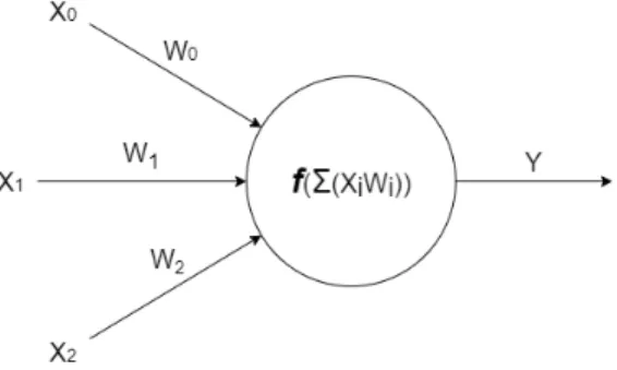
This section will explain the basic principles of neural networks, summarised by [5]. Neural networks are comprised of nodes, a sketch over a basic node can be seen in Figure1. Each node can be seen as a system that takes inputs and applies an activation function to it and outputs the result. Each node either takes inputs from previous nodes in the network or external sources. Every input into the node has a weight associated with it, this weight will determine how much of an impact that path has over the output.
Figure 1: A simple sketch over a single node in a neural network
The structure of a neural network often include layers which is what a block of nodes are called. There are generally three types of layers that can be in a network. There is the input layer that does not do any computation, it just takes in information from an outside source. The output layer takes the results from previous nodes and maps them to the desired output format. Finally, the hidden layers are the layers that are in between the input and output layers. It is in this layer that most of the computation occurs.
For a neural network to actually be useful it needs to be able to learn and adapt itself, so that when a certain type of data gets passed through it should output another type of data. For example, a network can be trained to classify if an image contains a cat or not. So in this case the image is the input to the network and the output will be a numeric value. To be able to learn this behaviour and many more, learning rules need to be applied to the system. These learning rules are mathematical logic that changes the weights in the network until the appropriate output is achieved.
There are different kinds of neural networks, the most basic one is the Artificial Neural Network (ANN). In this network, the input information flows through the network only in the forward direction. This means that the input goes through the input layer, hidden layers, and the output layer in that order and there are no loops or cycles.
Convolutional Neural Network (CNN) is a type of neural network that is specially designed to work with image data as input. CNNs are similar to ANNs in many ways, the feedforward structure is present in CNNs but it incorporates new layers that deal with the higher dimensions of an image. The most common layers added are convolutional and pooling layers which extract features from the image and condenses them into a ANN style network.
Another popular class of neural networks are the Recurrent Neural Network (RNN), which not only takes information from the current iteration of the network but also the previous iterations. This allows RNNs to have a temporal dimension unlike ANNs and CNNs that only considers a snapshot of time. Because of this temporal dimension RNNs are used with sequential data as input and at each instance it takes the previous data into consideration.
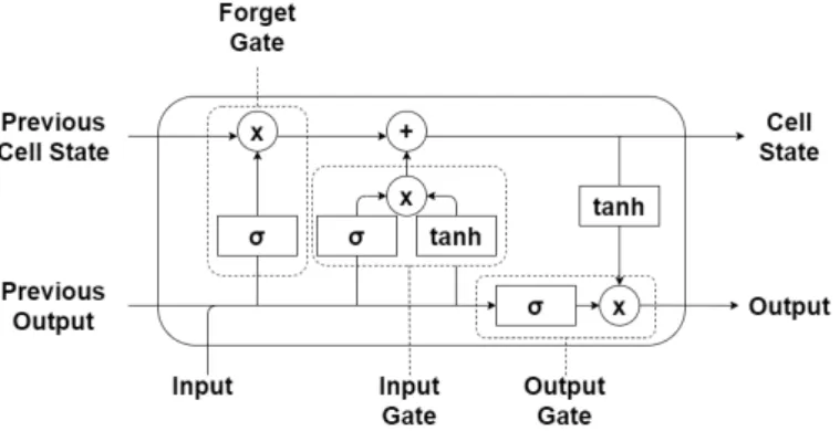
Long Short-Term Memory (LSTM) is one class of RNNs, LSTMs were created to deal with the short-term memory problem that simple RNNs suffer from. The short-term memory problem occurs when a RNN only takes information from the previous time step and adds it together with the current information, this means that simple RNNs start to lose information from the beginning that possibly is important. LSTMs combat this problem by introducing gates in the nodes that dictate what information is necessary and what information can be discarded. This makes LSTMs extremely good at processing long sequences [6].
Figure 2: Architecture over a LSTM cell and with its gates annotated
Another type of RNN is the Echo State Network (ESN), which is a form of reservoir computing. The basic structure of a ESN can be seen in Figure (3). The hidden layer in a ESN is called a reservoir and is made by having the connections and connection weights randomised between all of the nodes, instead of having connections between the nodes in an orderly manner. The idea is that the inputted sequence data will echo through the reservoir and in that way get a recurrent element. The biggest strength of ESN is the relative fast learning, This is because the weights in the reservoir are not trained and only connections to the output layer get trained[7].
Figure 3: Architecture over a ESN with the different layers annotated
2.2
Stereo vision
Stereo vision is a subset of computer vision where the disparity between two images is used to calculate depth in the image. A camera can be seen as a transformation tool that is used to project points in 3D space onto a 2D plane. The physical 2D plane is the sensor in the camera that captures the light coming through the aperture. The focusing of the camera lenses is how the light is projected onto the sensor. The 2D plane, referred to as the image plane, is easiest to
imagine as a virtual plane that sits in front of the camera. The plane captures the rays of light as points when they pass through the plane on their way into the camera.
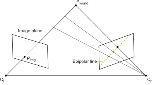
A line drawn between any world point and the camera will intersect the image plane in a point. Figure (4) show the intersecting line as ClPworldand the point of intersection as Pimg. The point
Pimg is the projection of the world point onto the image plane. Since the projection is from a
higher dimensional space to a lower one, some information is lost. The information lost in this case is the length of the line drawn from the camera to the point in 3D space.
Figure 4: The relation of points in world space to image planes of two cameras and the relation of the projected light path to the epipolar line in a second image plane. Where Clis the left camera
position and Cr is the right one
If two images each contain the representations of the same point in 3D world space from different viewpoints, the depth can be calculated using epipolar geometry. The problem is to find the corresponding points between the first and second image. It is by using the geometric relations between the two cameras positions and the point in world space that this problem can be simplified. The two camera positions and a point in world space span a plane called the epipolar plane. The lines at which the epipolar plane intersects the image planes are called the epipolar lines. As seen in Figure (4), the epipolar line corresponds to the projection line ClPworld. By searching along
these epipolar lines the corresponding points can be found. The epipolar planes for each world point will be rotated around the baseline ClCr. The resulting epipolar lines will all have different
orientations in the image planes. This makes the search for corresponding points difficult as it has to be done differently for each epipolar line.
The disparity between the corresponding points is related to the distance from the camera to the point in world space by the equation (1). The baseline b and the camera focal length f can be prior knowledge or attained by calibration. The disparity d is the difference in position between two corresponding points in each image. The depth z is the distance from the camera to a point in world space.
d = bf
z (1)
In practice, the problem can be simplified by placing two cameras parallel to each other and with a known distance between them. When the two image planes are parallel all epipolar lines become parallel as well. The problem of searching for corresponding points is reduced to a one-dimensional search. There can still be problems with finding corresponding points if the images do not contain enough distinct patterns that can be matched between the two images.
An image projector can be used to project a pattern of light onto the world. This structured light makes it possible to calculate depth when the scene itself does not contain good enough patterns to match corresponding points. An image projector has the opposite function of a camera,
but behaves the same for calculating disparity between an image and the image being projected. As such, it is possible to have a stereo vision system with only one camera and a light projector [8].
2.3
DC motors modelling
DC motors convert electrical power to mechanical rotation and are commonly used as actuators in robotic systems. A mathematical model can be developed in order to analyse aspects of a system containing DC motors. Rotation is induced in the rotor proportional to the voltage applied to the armature windings. The torque of the rotor is proportional to the current passing through the windings. The back-Electromotive Force (EMF) is proportional to the rotational speed of the rotor and acts against the voltage driving the motor. When the back-EMF is equal to the applied voltage the motor has reached its maximum speed. The relation for motor torque and back emf are shown in equations (2) and (3). Where the torque τ is equal to the motor torque constant Kt
times the current i. The back-EMF e is equal to the electromotive force constant Kb times the
angular velocity of the rotor ˙θ.
τ = Kti (2)
e = Kbθ˙ (3)
Since the SI unit for the motor torque and the back-EMF constants are equal, K can be used to represent both constants Ktand Kb. The modelling of a motor can be formed as in equations (4)
and (5), based on Kirchhoff’s voltage law and Newton’s 2nd law. Where J is the rotor’s moment of inertia. b is the viscous friction constant of the motor. L and R are the inductance and resistance respectively and V is the voltage applied to the motor.
J ¨θ + b ˙θ = Ki (4)
LdI
dt + Ri = V − K ˙θ (5) The systems transfer function is attained by first applying the Laplace transform, as seen in equations (6) and (7) expressed in terms of the variable s.
s(J s + b)Θ(s) = KI(s) (6) (Ls + R)I(s) = V (s) − KsΘ(s) (7) The final form for the transfer function is as shown in equation (8) where the input to the system is the voltage and the output is the rotational position of the rotor. This system is unstable and with a voltage input, it will grow unconstrained.
H(s) = Θ(s) V (s) =
K
s((J s + b)(Ls + R) + K2) (8)
With this model, it is possible to simulate systems actuated by DC motors to get an indication of how the system would behave if it was implemented with real-world components.
3
Problem Formulation
A robot that interacts with humans needs to be perceived as responsive and accurate, to make the person feel safe and comfortable with the interaction. This coupled with the fact humans cannot be expected to move and interact in a predefined way puts a lot of importance on the speeds of the actuators. Rapid dynamic changes in the target position require that the actuators are fast enough to keep up. Better performing actuators could mean a significantly higher hardware cost. A control system that could predict the movement of humans could react faster and compensate for slower actuators. The prediction could also make the interaction be perceived in a better way by making it more similar to an interaction between humans. In this master thesis, a method for predicting head movements in order to enhanced a control system is analysed and evaluated. A control system without predictive algorithm is compared to a system running with a predictive algorithm, to see if the prediction help slow actuator to keep up with erratic movement. A simulation of a robot arm is used to evaluate the two systems against each other, by seeing how close the robot position is to the ground truth when using prediction and when not using prediction.
3.1
Hypothesis
The hypothesis for this thesis, based on the problem formulation, is as follows:
If a robot can predict motion it will help the robot be more responsive and accurate with human-robot interaction.
3.2
Research Question
• RQ1: How well can a predictive algorithm anticipate real-world movements of a person?
• RQ2: What will the impact be of using a predictive algorithm in combination with tracking software compared to only using a tracking software?
• RQ3: In what way will the use of a predictive algorithm modify the system’s behaviour for actuators with different torque ratings?
3.3
Limitations
Evaluating the effectiveness of this work would ideally be conducted on a range of several state-of-the-practice and state-of-the-art actuator systems. However, this thesis work will only be evaluated with simulated actuators. Simulations are always an imperfect representation of reality. Any conclusions drawn from this work are only indications of the functionality on real systems or systems more complex than this work accounts for. Face detection will be done facing the camera in an environment that is well lit and has a uniform background. The focus of the work will be on AI methods, other prediction methods will only be tested if time is available.
4
Related Work
This section details a study of research that has been done in the field of Artificial Intelligence (AI) prediction algorithms for time series data. From the study, it can be concluded that the state of the art in this field are two types of RNNs namely LSTM networks and ESN.
4.1
ESN prediction
In the paper J.Zhao et al. [9] proposes an ESN with an adaptive lasso algorithm. Because ESNs consist of a reservoir that is sparsely and randomly connected it could lead to a collinearity problem if these reservoirs become very large. This means that some of the variables that should be independent are highly correlated. The adaptive lasso algorithm solves this problem by calculating the output weights. The proposed ESN was tested on one benchmark task and actual nonlinear time series. The results show that the network can reduce the computational burden and has a smaller error than other ESN models.
O.Adeleke [10] have developed a ESN for forecasting future levels of traffic in different networks. The ESN was compared to three other kinds of prediction models: LSTM, CNN and SARIMA. All of the models were tested on two datasets of data rates, the first dataset was made by collecting daily average data rates over 11 years and the second dataset contained the average data rates in 15-minute intervals over 96 hours. This is done so that both long-term and short-term prediction can be tested. Testing was done on a device with a 64-bit Intel(R) Core(TM) i7-4770 processor with a speed of 3.40GHz, and 32GB of memory running the Ubuntu 16.04 operating system. The results show that the proposed ESN achieved faster training and prediction times for similar levels of accuracy when compared to the other prediction methods.
ESN could be used in this thesis work as a means of predicting human movements. The relative fast training times could prove very useful because of the limited time in this thesis work. Both of the related works in this section shows that ESNs can accurately predict nonlinear time series. But the drawback is that it has only been used to predict single variables and not multiple variables which is of interest for this thesis work.
4.2
LSTM prediction
The work by R. Chellali and Li Zhi Chao [11] evaluated the use of LSTM networks to derive the final position and time for a human hand when performing a high five. The LSTM networks were trained using a dataset collected by having 10 different people do a high five motion towards a wall. The hand movements are saved as trajectories in 3D space which are then used in the LSTM networks. Three different parameters of the LSTM networks were tweaked and evaluated, The input sub-sequence length, the architecture, and the batch size. They concluded that that the prediction method generated so small errors that it could be useful for implementation on a real robot.
A vital part of human-robot interaction is for the robot to know where the human is located. In some situations it is even necessary for the robot to be able to make a prediction of where the human is. J.li et al. [12] tackles the problem of robotic sitting-to-standing assistance using a combination of model-based control and a LSTM to predict the humans intentions. A dataset was created by tracking the joints of human that would stand up from a sitting position using the help of another person. By training the LSTM it could predict if the human was going to stand up faster or slower or even sit down again, and the end-effector of the robot could be adjusted accordingly.
A.Alahi et al. [13] examined possibility to use LSTM to predict peoples trajectories when moving through a crowd of people. When moving through a crowded area people generally follow many unwritten rules based on social conventions. It is a complex task for a robot to understand these rules, but it would be valuable in a lot of applications where robots interact with humans. To incorporate the interactions between the different humans a LSTM is used to predict every individual’s x and y coordinates and then neighbouring LSTMs are connected via a pooling layer. Three proposed LSTMs were tested: one with the pooling layer, one with a simplified version of the pooling layer, and one without the pooling layer. The proposed LSTMs was tested with
four other methods on two publicly available human-trajectory datasets. Three metrics were used for comparing the Mean Square Error (MSE), final displacement error and average non-linear displacement error. It was concluded from the test data that the proposed LSTM outperformed the rest of the methods.
LSTMs have the advantage over ESN in that they have been researched more and therefore have been tested on more varied data. The data used in the related works described above is very similar to the type of data considered in this thesis work. The main similarity is that it relates to human movements and contains multiple variables that are tracked. The related work done by R. Chellali and Li Zhi Chao [11] is the one that is most similar to this thesis work.
5
Methodology
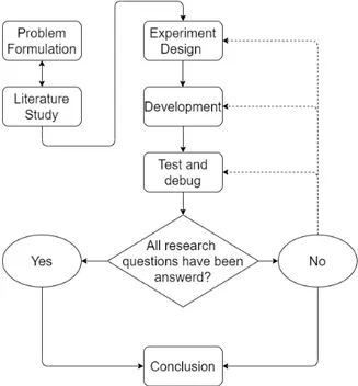
This thesis work uses a quantitative research method with a deduction approach to attempt to answer the research questions. Designing and implementing a proof of concept is well suited for an experimental method as the results can easily be quantified. This is commonly paired with a deductive approach in which experimental design can be guided by the hypothesis, which is why this method and approach was chosen [14]. The general process follows an engineering process outlined in [15]. The thesis work will follow the structure of the flowchart seen in Figure (5).
Figure 5: Flowchart over engineering process that is followed in this thesis work
5.1
Problem formulation
The problem formulation phase started by NEP providing a description over the problem that NEP wanted to be solved. After discussions with representatives from both Mälardalens Högskola (MDH) and NEP a problem formulation and research questions were derived.
5.2
Literature study
In this thesis work, the main focus of the literature study has been on finding the state of the art for prediction algorithms. What was of most interest was to find related work that closely matched the problem investigated in this thesis. Another big focus point has been searching and reviewing different databases, benchmark and simulation environments for the final testing of the algorithms. The face detection algorithms and depth measurement were not the main focus of the thesis and no new methods were investigated. For those parts it was not necessary for best algorithm and equipment to be chosen. They needed to be available on the market, be good enough to satisfy the goals, and be relatively easy to implement or acquire. From the literature study, an initial time plan over the development was created.
5.3
Experiment design
In the experiment design phase, everything that was going to be developed during the thesis work was decided upon. This meant that the algorithms which were implemented for the face detection and the prediction were chosen. The type of sensor that was used for depth estimation and data collection was also chosen together with the software environment for the simulation.
From the problem formulation and the limitations that were set, a suitable test environment and an experimental design were set up.
5.4
Development
Development phase was where everything was implemented. A dataset of 3D trajectories was created using data from a motion capture database. With the dataset collected a LSTM and a ANN was trained and evaluated. A tracking system was developed that could detect and track human head movements and save the trajectories. This system used the sensor setup to acquire the depth in images, and a pre-trained face detection algorithm which was implemented in MATLAB. To be able to answer RQ2 and RQ3 a simulation of a robot arm was implemented. Then the simulated arm was used with a tracking system with and without the prediction algorithms.
5.5
Test and debug
The test and debug phase and the Development phase were almost always happening parallel to each other. When one part finished in the development phase it entered the test and debug phase where it got debugged to see if the system or script was working correctly and then it got tested to see if it reached the goals for that task. If some part did not pass the test and debug phase it went back to the development phase and continued to get iterated over.
5.6
Thesis conclusion
Conclusions were derived from looking at the results from the simulations and the performance of the LSTM and ANN. The research questions were discussed and a conclusion for if they were fulfilled or not was made.
6
Method
This section outlines the methods that were chosen in order to answer the research questions.
6.1
Face detection
The method used for the face detection was a Multi-Task cascaded Convolutional Neural Network (MTCNN), which was proposed by K.Xhang et al. [16] for detecting faces and facial features. It later was implemented using the same weights as in [16] in MATLAB [17]. MTCNN is build up using three different CNNs that work in conjunction with each other. The first network is called the P-net which is used to obtain candidate bounding boxes for faces in the image. This information is then passed on to the next network called R-net. R-net takes all of the candidates and evaluates whether or not those bounding boxes contain a face. The last network is called the O-net and is design to describe the face in more detail by locating five facial landmarks: the eyes, the nose, and the corners of the mouth. This method was evaluated and produced good results on Face Detection Data Set and Benchmark (FDDB) [18], WIDER FACE [19] and Annotated Facial Landmarks in the Wild (AFLW) [20].
This method was chosen for this thesis work because it has been shown to have good accuracy while still maintaining real-time performance. The fact that it also detects facial landmarks was of great assistance for this work because it gives one point to track per landmark instead of having to rely on bounding boxes that include multiple points. To have easy access to an already trained and tested implementation of the method was another reason why this method was chosen.
6.2
Depth
Depth estimation was achieved by capturing images as stereo pairs. Semi-Global Matching (SGM) was used to find matching points in order to calculate a disparity map [21]. This method was used because it is implemented in the sensor hardware that was used. From the disparity map, the depth in the image was calculated using the camera parameters. The disparity was only calculated for the region where the face was detected which reduced the amount of uncertainty in finding the matching regions. This method was chosen because it allows for measurements over a large area without the sensor needing any moving parts. It can also easily be implemented in a system that already requires a camera. Both camera images and depth estimation can be done by using a stereo camera as a combined sensor system.
6.3
Simulation
A simulated model of a robotic arm was implemented to act as the actuated part of the system. A simulation allowed for the system to easily be evaluated in different configurations, such as with and without prediction algorithms. As well as changing actuators by simply changing parameters of the mathematical models. The simulation was set up to take a 3D trajectory as input and generate a trajectory of a robotic model’s end effector. By comparing how well the end-effector trajectory matches the input trajectory, for different configurations, the effects on the system’s performance could be shown.
6.4
Dataset
For the training and validation of the prediction algorithm, a dataset comprised of trajectories of human head movement in 3D space was needed. The dataset used in this thesis work was a motion capture dataset where humans performed different actions. The dataset tracked many different points on the humans in the dataset so one point for the head had to be extracted and stored [22]. The choice of a motion capture dataset in this thesis work stems from a lack of other types of publicly available datasets that fit the needs for this work. There exist quite a few datasets that film people doing different tasks and then labelling that action, putting a bounding box on it or adding body pose annotations [23][24]. But the problem with most of these datasets is that they do not contain the depth information that is needed.
6.5
Prediction algorithm
As a prediction algorithm, this thesis work implements a LSTM network and a simple ANN. The networks were trained and validated using the motion capture dataset. The reason for choosing LSTM for prediction was that during the research phase it could be shown that LSTM and ESN are state of the art prediction algorithms. But ESNs are mostly used for predicting only one variable at a time while LSTMs have been able to make multivariable predictions. The reason for also choosing a ANN is to have another baseline to compare the LSTM network with.
6.5.1 Dropout layer
When training a neural network a problem that needs to be addressed is overfitting. Overfitting is when a network learns too much about the noise and details in the training data and uses this information in the classification process. This will have a negative effect when the network is applied to more generalized data. To combat this effect, dropout layers were used in every network implemented in this paper.
Dropout layers work by randomly removing or dropping nodes and their connections in the network in every iteration. This will make the nodes less prone to co-adapt. One way of think about dropout layers is that during training multiple smaller networks are created and during testing, all of those networks get averaged out into the final sized network. Dropout layers have been tested on many various benchmark data sets and it has been concluded that dropout layers improve the performance of neural networks using supervised learning [25].
6.6
Hyper parameter optimisation
To optimise the Neural network hyperparameter settings for training a Particle Swarm Optimiz-ation (PSO) was used. The PSO algorithm was first proposed by Kennedy and Eberhart in 1995 [26]. The algorithm was inspired by multiple studies on animal’s social behaviours. These studies showed that certain types of birds communicating with each other when they wanted to find an optimal place to land. So the swarm of birds would spread out, look for a place to land, and by communicating start to conjugate around an optimal place to land.
In PSO a swarm of particles is used instead of a swarm of birds. Each particle can be represented by a vector X = [x1x2x3...xn] which is know as a position vector. The position vector contains
n a number of elements and each element represents one variable that may be optimised in the problem. The position vector can be taught of as the coordinates in an n-dimensional space wherein these particles move.
Each particle gets randomly placed inside of the n-dimensional space and evaluated using a fitness function f(X). After that, each particle adjusts its position according to its previous best positions and the best positions of all of the particles.
Besides a position vector, every particle also has a velocity vector that determines how the particle shall move through the search space each iteration. In the first generation, every particle starts with zero velocity, and then the velocity updates for every new generation. The velocity of every particle gets calculated by combing the particle’s previous velocity, the directional vector to the best personal position, and the directional vector to the best global position. A visual representation of this can be seen in Figure6. The velocity is calculated using equation9.
Vi(t + 1) =wVi(t) + r1c1(Pi(t) − Xi(t))
+ r2c2(Gi(t) − Xi(t))
(9) In equation9 V is the velocity vector, P is the best position for every individual particle, G is the best position of all particles, X is the current position, r1and r2vectors with random numbers
between 0-1 and c2, c1 and w are weights.
In 2002 M. Cleric and J. Kennedy [27] proposed the constriction coefficients, which will assign values for the weights c2, c1 and w, according to equation 10. The first step in the process is to
Figure 6: Calculating the next velocity of a particle in PSO
c1= χφ1, c1= χφ2, w = χ (10)
χ = 2κ |2 − φ −p
φ2− 4φ| (11)
In equation11κis constrained to 0 ≤ κ ≤ 1 and φ is constrained to be φ = φ1+ φ2≥ 4. The
final step is to assign values for κ, φ1and φ2. [27] set these values to φ1= 2.05, φ2= 2.05, κ = 1.
By using the this method to get the values of the weights it will help the PSO algorithm to converge to a local minima in a more precise way.
6.7
K-fold cross-validation
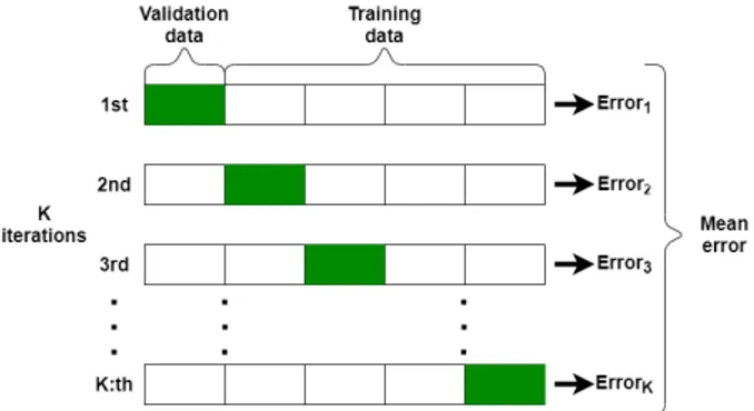
K-fold cross-validation is used to evaluate machine learning models when a limited amount of data samples are available. The main reason for performing cross-validation is to get a more accurate result on how the machine learning model will perform on unseen data. K-fold works by splitting the whole data set into K unique groups, then the first group gets selected as the validation set and the rest of the groups is set to be the training set. After the machine learning model gets trained on the training set it gets evaluated on the validation set. The next step is to shift the group that is the validation set to the second group and the rest is the training set. Now a new model gets trained and evaluated on the new sets. This continues until every group has been the validation set once, after that the mean error of all the runs is calculated and is the final score of the validation. A visual representation over K-fold cross-validation can be seen in Figure7
7
Ethical and Societal Considerations
This work used images to locate the position of a persons face. After the position was extracted, the image was discarded and no personally identifiable information about the person was saved. Additionally, a public database containing recordings of peoples head movements was used to train AI networks. This database also did not contain any personal information about the subjects. As such the methods used in this thesis does not make use of any data that requires ethical considerations.
The system described in this thesis may in the future be part of a commercialised product. Products that incorporate vision systems and face tracking have the potential for both a positive and negative impact on society. It could prevent people from accessing vehicles or machinery while under the influence of alcohol and contribute to making environments safer. It could also be implemented in a way where individuals movement could be tracked and personally identifiable information could be accessed in a way that would mean a violation of a persons privacy.
8
Experimental setup
In this section, the setup that was used to carry out the experiments and how the system was implemented is described. The section is structured broadly in the same way that the system operates. Starting with the acquisition of data using a sensor system and processing relevant to it. Followed by the setup of the AI algorithms used for prediction. The section ends by describing how the simulated part of the system was set up and the configurations used in experimentation.
8.1
Spatial face tracking
To allow the system to find the target position for the robotic model to move to, a subsystem that handled sensors and sensor data processing was implemented. The subsystem was responsible for reading data from the sensors, locating the face position from the data, calculate its 3D position, and output the series of 3D positions, representing the trajectory of how the face was moving in time.
8.1.1 Camera setup
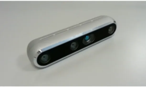
The sensor that was implemented to capture spatial data was the Intel RealSense D455 depth camera3, pictured in Figure8. The D455 is a combined sensor system containing a stereo camera,
an infrared (IR) projector, and an additional RGB colour sensor. It has a depth measuring range of 0.4 − 10 meters and a horizontal field of view of about 86 degrees [28]. The camera module enhances the depth measurement by projecting an infrared pattern that increases the texture in the scene.
Figure 8: Intel RealSense D455 camera
The D455 camera module was integrated with the control system by using MATLAB code wrappers of Intel RealSense SDK 2.04 functions. The wrapper functions were incorporated into a
MATLAB script that would handle the acquisition of data by capturing images, finding the face in the image, and calculating the depth to the face. Each iteration the script captures one colour image frame and one depth frame from the camera module. The depth frame contained the depth information for each pixel in the matching colour frame. The camera was configured for a frame size of 640x480 at a frame rate of 30 frames per second.
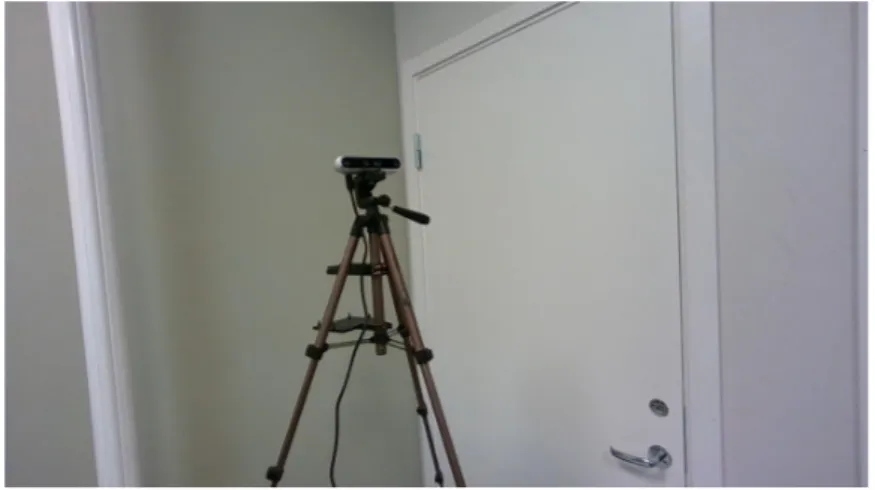
For the physical setup, the camera was mounted on a tripod at face height, approximately 1.75 m from the ground, as shown in Figure9. Measurements were acquired with a person facing the camera and moving in a span of 0.5 − 2 meters in front of the camera.
8.1.2 Face detection
Each image frame captured by the camera was passed to the MTCNN function in MATLAB. The face detection function returns a bounding box of the face position in the image. The position of the bounding box was used to find the corresponding position of the face in the depth frame. Distance to the face was calculated by taking the average value of all points within the bounding
3https://www.intelrealsense.com/depth-camera-d455/ 4https://github.com/IntelRealSense/librealsense
Figure 9: Physical camera setup
box. The value was then adjusted by subtracting 10 cm to ensure that the target position would be in front of the face.
8.1.3 Trajectory alignment
With the faces position known in the image and the depth being calculated, the position could be transformed from pixel coordinates to world coordinates. The camera parameters specific to the used D455 were calibrated from the factory and read directly from the cameras internal memory. The camera matrix K in eq. (12), was the matrix that the pixel coordinates [u v 1] was multiplied with to transform them to world coordinates of [x y z 1]. With the points created as having x and y aligned with the image plane and z being the distance from the camera, another transform needed to be applied to align the points correctly with the world coordinate system at the base of the robot. The transformation matrix M in eq. (13) made it so the trajectory points were aligned with z being the height from the floor and y being the distance from the camera to the person.
K = 380.7371 0 312.5167 0 379.9458 242.0441 0 0 1 (12) M = 1 0 0 0 0 0 −1 1 0 1 0 1.75 0 0 0 1 (13)
8.2
Data manipulation
Before the training data can be used to its full potential, pre-processing of the data needs to be done.
8.2.1 Motion capture
The dataset that was used for training and validation was collected from Carnegie Mellon University motion capture library [29]. There are several different motions collected from the motion capture library and some of them did not make sense to use in the dataset. Some examples of excluded motions were people pretending to be animals, people signing, people break dancing and people sitting on a stool. This meant that the motions that were going to be in the dataset needed to be handpicked. To avoid the models only training on one particular type of head motion a variety of different types of motions were selected. Some examples of motions in the dataset is people walking, people washing a window, people kicking a football and people boxing. A full list of the exact files used can be seen in the appendix in Table9.
Since the motion capture dataset contains multiple tracking points across the whole body of the subjects, a function needed to be implemented to extract only the tracking points on the head. These points get averaged into one trajectory which is then exported and used as input data for the neural networks.
8.2.2 Velocity and acceleration calculations
To get more information out of the dataset trajectories, the velocity and acceleration of each position were estimated. The velocity was estimated in every axis and was done by subtracting the previous position to the current position and dividing by the time between them. Similarly, the acceleration was calculated using the 1st order derivative. By doing this each position in the dataset generates nine input values.
8.2.3 Standardising the data
To prevent any scaling issues when training the dataset is standardised to have zero mean and unit variance. This is accomplished by calculating the mean and standard deviation, then subtracting the mean from the dataset and dividing it by the standard deviation.
8.3
Network architecture
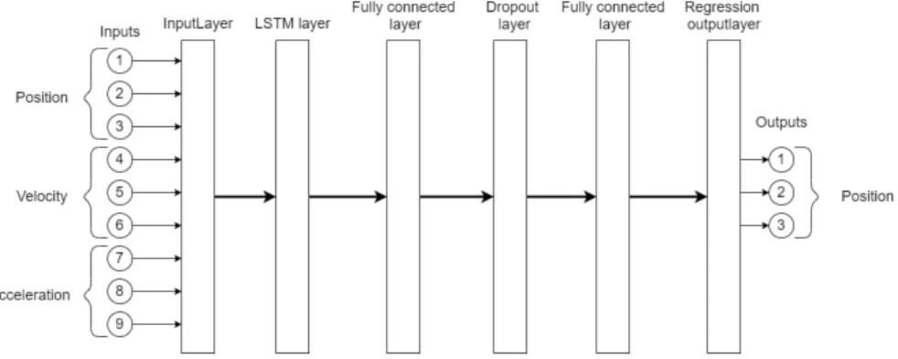
Two types of neural networks were implemented and tested for prediction purposes. All of the networks have been coded and trained in MATLAB and MATLAB deep learning toolbox. A basic architecture over a LSTM network were devised, which can be seen in Figure 10. This basic architecture was altered and optimised for different prediction times by a PSO algorithm. The PSO determined the number of LSTM layers and fully connected layers before the dropout layer and also how many nodes each layer has.
The basic architecture of the ANN is almost the same as the LSTM but without the LSTM layer. When optimising the architecture it can still change the number of fully connected layers and the number of nodes in each layer, but it can also change how many inputs there should be. Because the ANN does not consider the time aspect that the LSTM have, in most cases it requires more input data to make an accurate prediction. As the positions generate nine inputs so the input size of the ANN is always a multiple of nine.
Figure 10: Basic architecture over a LSTM network
8.4
Hyper parameter optimisation
When a general structure of the LSTM network and the ANN was established and tested to verify that results were adequate, a PSO were deployed to optimise the training parameters and structure parameters of the two neural networks. The two networks were optimised four times each with different prediction times (how far in the future the network should predict). The four different prediction times were defined as 1/2 of a second, 1/4 of a second, 1/8 of a second and 1/16 of a second.
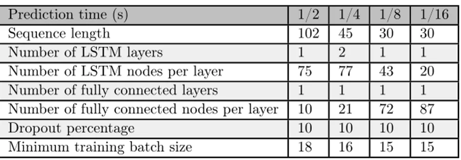
The parameters that get optimised differs between the two networks. The parameters for the LSTM are listed in Table1. The "sequence length" parameter refers to how many samples there should be in every sequence. "Dropout percentage" is how high the percentage of the dropout layer should be set to. The "Minimum training batch size" defines the number of sequences that will be propagated through the network during training.
The ANN has almost the same parameters optimised as the LSTM, but it does not need to change the parameters that are about LSTM, but it needs to change how many coordinate points get input. All of the parameters that are optimised for the ANN can be seen in Table2.
Prediction time (s) 1/2 1/4 1/8 1/16 Sequence length 102 45 30 30 Number of LSTM layers 1 2 1 1 Number of LSTM nodes per layer 75 77 43 20 Number of fully connected layers 1 1 1 1 Number of fully connected nodes per layer 10 21 72 87 Dropout percentage 10 10 10 10 Minimum training batch size 18 16 15 15
Table 1: Optimised values for LSTM
Prediction time (s) 1/2 1/4 1/8 1/16 Sequence length 33 34 92 162 Number of input points: 33 11 3 1 Number of fully connected layers 6 2 1 1 Number of fully connected nodes per layer 26 42 12 43 Dropout percentage 38 10 10 10 Minimum training batch size 19 18 22 23
Table 2: Optimised values for ANN
8.5
prediction error evaluation
A 5-fold cross-validation was implemented to acquire a more accurate result on how the neural network models would work on unseen data. A total of 122 different 3D trajectories was used as the dataset. These were randomised and divided into 4 groups with 25 trajectories each and one last group with 22 trajectories. The models are trained on the four of the groups and then validated on the last. Each group is validated once and then the mean error of the 5 runs gets calculated.
To have a baseline to compare the prediction error of the LSTM and ANN with, three non-AI methods are also evaluated for the different prediction times. The first method is the most basic and is to assume that there is no movement of the position and predicts that the output position is the same as the input position. The next method assumes that the input position will continue with its current velocity constantly for the duration of the prediction time and concludes that that position will be the output position. The final non-AI method is the same as the second method but instead of assuming a constant velocity, it assumes a constant acceleration.
8.6
Simulation
Following is a description of each model used in the simulation as well as how the evaluation was implemented. The simulated robotic part of the system consisted of a combination of several mathematical models. These models describe how the dynamic part of the system behaves during simulation run time. The simulation was conducted by evaluating the models for each point of sensor data. Input data to the simulation was received directly from the camera sensor subsystem. The time steps were specified by the sample rate of the sensor system.
8.6.1 Robotic model
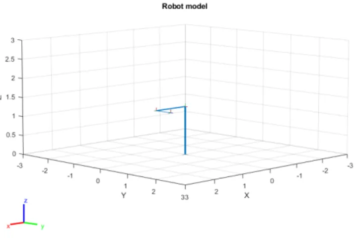
The robot model was set up as a three Degrees of Freedom (DOF) Cartesian robot arm. The orientation and positions of the joints were implemented by defining a rigidbodytree in MATLAB using the Robotics System Toolbox. Figure11 shows the model in a random configuration. Para-meters for the rigidbodytree were specified using the Denavit–Hartenberg convention. A matrix containing the parameters was created, as shown in eq. (14). Each row of the matrix represents the parameters in the order [riαidiθi].
Figure 11: Robot model drawn for a random joint configuration.
The design of the robot was kept generic in order for the control system to be easy to adapt to a physical prototype, that may be built at a later time. The implementation as a Cartesian robot was requested by NEP and lead to the robot being modelled with three prismatic joints. Because all the actuators were linear they were set up to control movement in one Cartesian axis each.
DH = 0 π/2 d1 π/2 0 π/2 d2 π/2 0 0 d3 0 (14) 8.6.2 Joint model
All the joint of the robot were modelled using the transfer function in equation (8). The transfer function takes a voltage as input and outputs the rotational position. In a robotic joint, it is most useful to control the joints by specifying the desired position for the joint and use a control loop to move the joint to the correct position. This was achieved by adding a Proportional-Integral-Derivative (PID) controller and making each joint a closed-loop control system as seen in Figure12. The PID controller takes the error in position as an input and outputs the voltage required to move the motor to the correct position. The reference input Desired position was either the trajectory captured by the camera or the trajectory obtained from a prediction algorithm, depending on the configuration.
To convert the output of rotational position to linear position for the prismatic joints, the conversion ratio was assumed to be 1 : 1 and without friction.
8.6.3 PID controller
A PID controller was used to move the joints to a given input position. The parameter values for the controller were set so that the controlled system had a crossover frequency of 10 Hz and a phase margin of 80 degrees. The values used were Kp = 3.56, Ki = 6.6, and Kd = 0.0619 and
Figure 12: Diagram of closed loop joint controller
was obtained from the pidtune function of the Control System Toolbox in MATLAB. These values were used to get the base performance of the system.
8.6.4 System validation
The tests were conducted by having a person face the camera and move in a pattern while the system captured a trajectory. The person approached the camera from a two-meter distance and stopped at one meter from the camera. The person then moved perpendicular to the camera for one and a half meters on either side. The person continuously varied the speed and direction of the face’s movement in a two decimetre radius. The procedure was repeated three times to gather data for evaluation. The prediction algorithm received the captured trajectory as input. The captured data was also linearly interpolated to match the theoretical sample rate of the system given by the settings in section8.1.1. The simulation was tested with and without interpolated data.
The simulation was made to simulate two systems for each run. One was the system running with predictive algorithms and the other without prediction. The two setups were iterated through several version of the motor transfer functions, defined by a set of motor parameters, as shown in Table 3. The parameter values for the DC motor model was derived from the manufacturer specifications [30]. DC motor ID 1 2 3 4 5 6 7 8 9 10 Rated torque (Nm) 0.883 1.765 2.189 2.542 3.037 4.096 6.038 7.838 16.948 24.716 Moment of inertia (kg.m2) 1.55 · 10−5 2.83 · 10−5 3.67 · 10−5 4.59 · 10−5 5.51 · 10−5 2.1 · 10e−4 2.97 · 10−4 3.88 · 10−4 1.5 · 10−3 2.2 · 10−3 Viscous friction (N.m.s) 4.07 · 10−4 8.30 · 10−4 1.96 · 10−4 2.38 · 10−4 2.84 · 10−4 3.89 · 10−4 2.58 · 10−4 7.43 · 10−4 1.2 · 10−3 1.3 · 10−3 EMF (V/rad/sec) 0.0191 0.0342 0.043 0.0517 0.062 0.08 0.06 0.05 0.275 0.3533 Torque constant (N.m/Amp) 0.0191 0.0342 0.043 0.0517 0.062 0.08 0.06 0.05 0.275 0.3533 Electric resistance (Ohm) 0.6 0.7 0.54 0.63 0.56 0.43 0.14 0.15 0.62 0.6 Electric inductance (H) 3.50 · 10−4 5.00 · 10−4 7.20 · 10−4 7.70 · 10−4 9.70 · 10−4 9.00 · 10−4 2.40 · 10−4 1.80 · 10−4 2.00 · 10−3 2.00 · 10−3
Top speed (rad/sec) 492 241 204 168 141 282.74 466 188.5 121 133
9
Results
This section presents the results from the experiments carried out. The section is divided into three parts, The first part shows a comparison of the different prediction algorithms. The second part show results from experiments using the prediction algorithm in a simulated environment, and the last part contains results from comparing different actuators in the simulated system.
9.1
Prediction network
Table4 Shows the prediction errors of all of the different algorithms and for the different predic-tion times. Figure13 is a visual representation of how the predictions change depending on the prediction time, which shows four 3D graphs of a validation trajectory and the LSTM and ANN predictions for this trajectory. Each graph corresponds to a different prediction time, in A the pre-diction time is 1/2, B is 1/4, C is 1/8 and D is 1/16 second. To make it easier to see the difference between the two AI methods Figure14shows a trajectory and the corresponding predictions split up into X, Y and Z axis. In this example, the prediction algorithms try to predict 1/4 of a second into the future. Figure15is the same sort of figure as Figure14but over another trajectory and the prediction time is 1/16 second.
Prediction time (s) 1/2 1/4 1/8 1/16 No prediction (mm) 167.56 92.86 48.38 22.86 Velocity prediction (mm) 141.16 57.09 22.56 8.74 Velocity and acceleration
prediction (mm) 391.89 107.47 32.99 11.24 LSTM (mm) 141.20 74.93 43.46 47.69 ANN (mm) 154.76 77.14 34.63 17.91
Figure 13: Graphs over a 3D trajectory from the validation set with the correlated prediction trajectory for 4 different prediction times. A is over a prediction trajectory where the Neural networks try to predict 1/2 of a second into the future, B is for 1/4 of a second, C is for 1/8 of a second and D is for 1/16 of a second.
Figure 14: Graphs over trajectory from the validation set split up into X, Y and Z axis. The neural networks is trying to predict 1/4 of a second in the future.
Figure 15: Graphs over trajectory from the validation set split up into X, Y and Z axis.The neural networks is trying to predict 1/16 of a second in the future.
9.2
System integration
This section contains the result gathered while performing the experiment as described in the experimental setup section. In Table 5 and Table 6 are summaries of the measured numerical results shown for different setups. The columns represent prediction time from 1/16 to 1/2 second. The tables contain results for when the reference input to the closed-loop control system was the prediction from different algorithms. The results for No prediction are based on when the reference input came directly from the camera sensor system. The results are then repeated for the LSTM and ANN setups but with interpolated input.
Table5presents the error, calculated as the Euclidean distance to the desired position, average over the experimental runs. Table6 shows the percentages of run time where prediction resulted in a trajectory that was closer to the desired trajectory than without prediction.
Prediction time (s) 1/2 1/4 1/8 1/16 No prediction (mm) 47.64 47.64 47.64 47.64 LSTM (mm) 169.85 104.10 89.46 66.26 ANN (mm) 264.59 200.50 122.09 87.62 Velocity prediction (mm) 193.00 111.84 59.73 47.02 Velocity and acceleration
prediction (mm) 284.69 128.20 62.02 49.41 Interpolated No prediction (mm) 40.79 40.79 40.79 40.79 Interpolated LSTM (mm) 114.09 53.42 64.59 47.19 Interpolated ANN (mm) 176.93 91.41 57.52 48.40
Table 5: Resulting error from simulation as Euclidean distance from target position. Prediction time (s) 1/2 1/4 1/8 1/16 LSTM < No prediction (%) 2.45 8.58 11.86 23.15 ANN < No prediction (%) 1.12 2.07 3.82 3.87 Interpolated LSTM < No prediction (%) 18.85 33.8 27.30 38.86 Interpolated ANN < No prediction (%) 2.69 9.55 17.49 16.33 Table 6: Proportion of duration where prediction results in smaller error.
The average reduction in error from non-interpolated to interpolated data is seen in Table 7. Table 8 show the factor of gain in performance from interpolated data based on the values in Table6.
No prediction (%) 14.38 LSTM (%) 34.52 ANN (%) 46.30
Table 7: System error reduction from interpolated data. Prediction time (s) 1/2 1/4 1/8 1/16 LSTM factor 7.69 3.94 2.30 1.68 ANN factor 2.40 4.61 4.58 4.22
Table 8: LSTM and ANN performance gain from interpolated data.
The sampling rate of the sensor system averaged 6.3 data points per second. The low sampling rate resulted in the prediction algorithms getting 5% of the 120 Hz that the training dataset was captured with. The camera settings used allowed for a theoretical sampling rate up to 30 Hz.
Figure 17 shows the difference between the prediction results for the base sample rate and the interpolated sample rate, for movement recorded in the X axis at 1/4 second prediction time.
Figure 16: Results of simulation based on LSTM prediction compared to simulation result for no prediction. A is for 1/2, B is for 1/4, C is for 1/8, and D is for 1/16 second.
Each simulation resulted in a trajectory representing the path of the robot’s end effector. The trajectories generated from the system with predictive algorithm and different prediction times can be seen in Figure 16. The input trajectory is the desired position that all simulated trajectories are compared against.
Figure18shows the results of all prediction times in the same graph. It is focused on an event where the face rapidly changed position along the X axis.
In the LSTM example, there is a difference in behaviour for the trajectories that were simulated with input generated by prediction. The simulation based on the no prediction input is always behind the desired position in time. The prediction based trajectories rise before the input and also goes down before the input. It can also be seen that for parts where no or very slight movement occurs, the prediction based trajectories becomes unstable when longer prediction times are used. For the ANN the events occur at different times because part of the input trajectory was cut at the beginning to give the ANN inputs to start prediction.
Figure 17: A show the LSTM prediction result for 1/4 second with 6 Hz sampling. B show result for interpolated 30 Hz sampling rate.
Figure 18: Simulation result for a local region in the X axis input with all simulated prediction times. Subplot A contain LSTM results and B the ANN results
9.3
Actuators
For every time that the robot was simulated, the actuator model was evaluated for the motor parameters described in section8.6.4. Important to note is that the motor ID is ordered based on ascending torque value. Performance was measured by how often the simulated trajectories with prediction were closer to the desired position, than when compared to the simulated system without. This was measured for each of the ten actuator models. The values were saved as percentages of simulated time where prediction resulted in a more accurate trajectory. Figure
19shows the data points for each prediction time normalised to have zero mean and a standard deviation of one. The lines are fitted to each set of data points using linear regression.
The slope of the lines shows the performance of the prediction algorithms, in comparison to the system without prediction, depending on the torque of the motor model that was used in the simulation. The difference in slope shows how increased prediction time alter the way the system’s performance changes with an increase of motor torque.
Figure 19: Performance of actuator models for each prediction time plotted with zero mean and a standard deviation of one. Lines fitted using linear regression show the data trend as torque increases with motor index.
10
Discussion
In this section the results from section9 are discussed. This section follows the same structure as section 9, First results about different prediction algorithms are discussed, secondly results about prediction algorithm in a simulated environment and lastly results about comparing different actuators are discussed.
10.1
Prediction network
When observing the result from the 5-fold cross-validation in Table4 it can be seen that making a prediction from the velocity and not using any AI is the best method across all 4 prediction times. One reason for this seems that both AI methods have a hard time making predictions when there is small or no movements and tends to fluctuate around the correct value, this can be seen in Figure14and Figure15. From Table4 it can also be concluded that predicting using velocity and acceleration is the worst method for 1/2 and 1/4 second but performers decently for 1/8 and 1/16. This is because from 1/4 second and higher the acceleration can change drastically which will result in poor predictions.
From the Table 4 it can be seen that the LSTM network outperformed the ANN for the two longer prediction times but was worse on the other two. And is severely worse for 1/16 second. These results can also be seen in Figure15, The graphs in the bottom right show that for 1/16 the LSTM fluctuates around the correct value more than the ANN. But for all prediction times other than 1/16 both AI methods performed similarly when just comparing the raw prediction error.
Figure 13 shows how the different prediction methods converge to the real result when the prediction time gets shorter. For a prediction time of 1/2, the prediction algorithms have trouble predicting the fast moments but can still follow the path roughly. When looking at 1/4 second improvements from 1/2 second are really clear to see, now both the LSTM and the ANN stays relatively close to the actual motion even in quick movements. For 1/8 and 1/16 both methods stay even closer to the trajectory than it does for 1/4.
The no prediction category in Table4can also be seen as a measurement of how far a position moves on average for the different prediction times. This gives a good baseline to compare the prediction methods too. It can be concluded that both LSTM and ANN performs better than using no prediction for all cases but one, that is where the LSTM tries to predict 1/16 of a second.
10.2
System integration
By examining the results presented in Table 5, a few observations can be made regarding the performance of the implementation of the control system as a whole. Firstly, the simulated part of the system evaluates the robotic controller model based on the discrete time steps of the input data. This means that the no prediction control system increase performance when the input data is interpolated to contain a greater number of data points. This is to be expected as the simulation is evaluated for shorter time steps and thus can react faster to the changing input. The system also gains a substantial increase in performance from interpolation for both predictive AI algorithms that were tested. In Table7it can be seen that the no prediction system had a 14.38% reduction in the average error. The system using the LSTM and ANN algorithms each see a 34.52% and a 46.30% reduction in the average error, averaged over all four prediction times. This shows that the predictive algorithms would perform significantly better with a higher sampling rate. A comparison between the interpolated prediction and the base prediction is seen in Figure17. The graphs clearly show how the interpolated prediction for the longer prediction time achieves a better result.
The prediction methods based on velocity and acceleration are shown in Table5to have better results than the AI algorithms for short prediction times. The LSTM show a better result for 1/2 and 1/4 second prediction. This result can be expected because a shorter prediction time more closely resembles a linear problem. For longer prediction times the prediction needs to take the curvature of the trajectory into account. Velocity and acceleration prediction only has information about the change from the previous point to the current.