Biofuels production versus forestry in the
presence of lobbies and technological change
Johanna Jussila Hammes
Swedish National Road and Transport Research Institute, VTI
Box 55685; SE-10215 Stockholm
Tel: +46 8 555 77 035; E-mail: johanna.jussila.hammes@vti.se
July 8, 2009
Abstract
We study the political determination of a hypothetical land tax, which internalises a negative environmental externality from biofuels. The tax allocates land from biofuels towards forestry. Lobbying af-fects the tax rate, so that the sector with the lower elasticity of land demand determines the direction in which the tax deviaties from the social optimum. Lobbying by the sector with higher elasticity of land demand cancels partly out the other sector’s lobbying. The politically optimal tax rate is "self-enhancing" in that the tax lowers the elastic-ity of land demand in the sector which initially had a lower elasticelastic-ity,
This is the modi…ed …rst chapter of my PhD thesis from the University of Gothenburg. I thank Per Fredriksson, Toke Aidt, François Salanie, Jason Shogren, Svante Mandell, Jan Erik Nilsson and Klaus Hammes for valuable comments. All remaining errors are my own.
and raises it in the other sector. This can dwarf the government’s other attempts to support the production of biofuels. Finally, techno-logical progress in biofuels serves to strengthen that sector by lowering its elasticity of land demand, and weakens the forestry sector by rais-ing its elasticity of land demand. Dependrais-ing on the initial tax rate, this can be welfare enhancing or lowering. Furthermore, it can lead to excessive deforestation.
Keywords: Biofuels, forestry, land use, political economy, technological change
"This paper has not been submitted elsewhere in identical or similar form, nor will it be during the …rst three months after its submission to the Publisher."
1
Introduction
Production and use of biofuels, both for electricity and heat generation and for transportation, has grown over the past years. There are many reasons for this, among other climate change, energy security, high fossil fuel prices and rural development goals. Production of most types of biofuels requires land, however, thus competing for land both with agriculture and with forestry.1 For instance, Hyytiäinen et al. (2008) …nd for Finland that the production of biofuels (reed canary grass) is the most pro…table use of arable land (com-pared to growing oats or pine trees), although only in the proximity of (at most 40 km from) a thermal power station. Lankoski and Ollikainen (2008) in turn …nd that production of reed canary grass in Finland, when the alter-native is oats, is socially optimal even 100 km away from the power plant. In the tropics, not only fallow or unused agricultural land is used for biofuel production but also rainforest land has been converted, for instance, to palm oil plantations.2 This development is largely driven by policy measures, for
instance, by the European Union’s (EU) 20-20-20 target (a reduction of at least 20% in greenhouse gas emissions, and a 20% share of renewable energies in the EU’s energy consumption by 2020), set by the European Council in March 2007.
Biofuel production may, however, lead to negative side e¤ects. According to (WWF, 2008, 3),
depending on which crops are produced, where and how, bioen-ergy developments can cause signi…cant negative environmental and social impacts, including deforestation, biodiversity loss, soil
erosion, excessive water use, con‡icts over land rights and land use, food shortages and staple food crop price spikes.
It is further conceivable that biofuel production that replaces forestry increases the use of fertilizers, pesticides and herbicides, thus increasing the run-o¤ of these to the surrounding nature and waterways.
It is thus possible that land use change towards the production of biofuels, especially if biofuel production replaces forests, creates a negative external e¤ect compared to land use for forestry. Although several di¤erent external e¤ects are present, the common thread is the change in land use. Therefore, if a government wanted to internalise the externality using only one policy instrument, taxing land use for biofuel production would be a …rst-best policy instrument. It is, however, possible that lobbying by the sectors involved a¤ects the setting of such a tax rate.
The aim of this paper is to contribute to our understanding of the process of land use change between forests and biofuels, how it is regulated, and how the political economics behind this process work. We do this by examining three factors that can in‡uence such a process. We start by assuming that the government imposes a land use tax on the biofuels producing sector, in order to internalise the negative externalities that it produces.3 However, lobbying,
and government susceptibility to lobbying, have an impact on the level of this policy instrument. This in turn a¤ects the allocation of land between the two sectors. It is futher possible that government policies change the strength of the two lobby groups, the biofuels and the forestry lobby, respectively. We examine both how a land tax on biofuels and an (exogenous) biofuels target
or other such policy which aims to boost the production of biofuels a¤ect the lobby groups’strength.
Finally, we study the e¤ect of an (exogenous) improvement in the technol-ogy of growing biofuels, and how this a¤ects the two lobby groups’strength, and the optimal land use. The cause of technological progress is unspeci…ed and can take the form of better varieties of crops, increased fertilizer, pesti-cide or herbipesti-cide use or other changes. If a small country is able to export at a given price, then an improvement in the technology, by increasing the productivity of land in biofuel production, increases demand for land for bio-fuels and thereby leads to deforestation. What we add is a description of how lobbying a¤ects this land reallocation.
The present paper touches several di¤erent branches of economic inquiry. Thus, studies of optimal land allocation between two sectors have mainly con-centrated on studying land allocation between agriculture and forestry, and the mechanisms behind deforestation. The question has mainly been seen as a dynamic resource use problem. Among others, Ehui and Hertel (1989) and Ehui et al. (1990) calculate the optimal steady-state forest stock, and exam-ine also the e¤ect of other factors, such as technology, fertilizer use or social discount rates. Barbier et al. (2005) study the cumulative level of resource conversion and examine how trade policy in‡uences the distortions created by political corruption. Their empirical …ndings suggest that increased cor-ruption and resource dependency promote land conversion, whereas rising terms of trade reduce conversion of forestland to agriculture.
While the literature on biofuels is rather young, it is growing fast. It has mainly concentrated on examining the e¢ ciency of various policy
in-struments in supporting the expansion of biofuels production,4 and more
recently, the implications of biofuels production on the environment,5 and
the food supply.6
Land taxes have been studied extensively in the past, although the re-search has concentrated on the e¤ect of land taxation on economic growth.7
Land taxes as an instrument for environmental policy is largely missing from the literature. This might be partly due to the fact that land taxes rarely exist in reality (Lindholm (1979)). Plausible explanations as to why this is so are (to our knowledge) missing from the literature.
By way of including lobby groups that attempt to in‡uence the govern-ment’s policy, this article o¤ers an explanation to the rarity of land taxation, and even to the fact that land use for e.g., agriculture is often subsidised rather than taxed. The motive for land taxation here di¤ers from that in the traditional literature, however, where it is seen as a tool to raise revenue and to encourage economic growth. Thus, we formulate a political economy model of a land tax aimed at internalising a negative environmental external-ity arising from land use by the biofuels sector in a setting where two sectors, biofuels and forestry, use land in production. Unlike in the "traditional" land tax literature, there is no revenue motive for taxation. Furthermore, it is pos-sible that lobbying turns the "tax" into a subsidy. The model is based on Bernheim and Whinston (1986) principal-agent model with menu auctions, which Grossman and Helpman (1994) extend to trade policy formation.
Grossman and Helpman’s model has by now spawned a large literature examining environmental policy determination.8 The contribution of the
equilibrium e¤ect arising from competition for, and a change in a factor use arising from the introduction of the policy instrument. Thus, both the biofuels and the forestry sectors use land in production and compete for it, and land use by neither sector is …xed.9 This innovation allows us to
study endogenous change in lobby group strength and to adjust factor use endogenously.10
We further examine the e¤ect of land augmenting technological change in the biofuels sector, and its consequences for lobby group strength and wel-fare. Technological chage raises the productivity of land thereby leading to an increase in its value, given constant output prices, and resulting in land reallocation from the less towards the more productive sector. This corre-sponds for instance to Ehui and Hertel (1989), who show that technological progress in agriculture lowers the optimal steady-state forest stock. In the present article, we show how technological change also works to strengthen the (technologically) improving sector’s lobby group vis-á-vis the government compared to the stagnant sector, and how this leads to increased pressure to lower the land tax rate and the allocation of land between the sectors.
The paper is organized as follows: In Section 2 we present the formal model and discuss changes in land use due to land taxation. Section 3 dis-cusses the tax rate, and 4 analyses the lobby groups’strength and strategies. In Section 5 we study the e¤ect of technological change on the lobby groups and on land allocation. The …nal section concludes.
2
The Model
Consider a small open economy where the output prices of goods are treated as exogenous. In other words, we assume the existense of a world market both for biofuels and for wood, which sets the world market price for these goods and that the world market prices also apply domestically. The economy is assumed to consist of N individuals with identical, additively separable preferences. We normalize N = 1 without loss of generality. Each individual maximizes a utility function of the form Uh = x
O+Pi=B; Fui(xi) (TB),
where xO denotes consumption of a numeraire good O and xi consumption
of biofuel and logs, which will be indexed by i; j 2 fB; F g, i 6= j. The sub-utility functions ui(xi) are di¤erentiable, increasing and strictly concave.
The net damages from land use for biofuels production, (TB), where TB
is land use by the biofuels sector, are di¤erentiable, increasing and strictly convex. Land use in the forestry sector F , TF, is assumed not to cause any
(net) externalities.
The numeraire good O has a domestic and world market price equal to one. The domestic and world market price of biofuels and logs equals pi. With these preferences each consumer demands di(pi) units of good
i, where di(pi) is the inverse of the marginal utility function u0i(xi). The
remainder of a consumer’s income E is devoted to the numeraire good. The consumer thus attains indirect utility given by v (p; E) = E +S (p) (TB),
where p (pB; pF) is the vector of output prices of the non-numeraire
goods and S (p) = Pi2fB; F gui[di(pi)] Pi2fB; F gpidi(pi) is the consumer
no consumer surplus.
The numeraire good O is produced using labor alone, with constant re-turns to scale and an input-output coe¢ cient equal to one. We assume that the aggregate labor supply, l, is su¢ ciently large to ensure a positive output of this good. It is then possible to choose units so that we can set the wage rate to one (w = 1). Goods B and F are produced using labor and land, also with constant returns to scale. The aggregate rent accruing to land in sector i =fB; F g is denoted by i(pi; zi; Hi), where Hi is a technology parameter
on land use (Romer, 2001, 9) and zi is the cost of land.11 Hotelling’s lemma
gives the industry’s land demand curve @ i
@zi = Ti. Because a change in land
price, and consequently, land demand, also a¤ects sector j, we further obtain a general equilibrium e¤ect on that sector’s land demand: @ j
@zi = Tj
@zj
@zi.
Allocation of land between the sectors is not …xed but land demand Ti
is a function Ti(pi; zi; Hi). For simplicity, we assume land demand to be
falling but linear in land price, so that @Ti
@zi = Ti2 < 0, Ti22 = 0 and Ti23 = 0.
The production function of good i is given by yi yi(HiTi; Li), where Li is
labor demand.12
The government has only one policy instrument at its disposal, namely a land tax or subsidy on the biofuels sector. Since the tax is used to internalize a negative externality arising from land use, it is the …rst-best policy instru-ment. Revenue from the tax (cost of the subsidy) is distributed (collected) in a lump-sum fashion to the consumers.13
The ad-valorem land tax/subsidy drives a wedge between the value of land z and the cost of land to the biofuels sector, zB. The tax/subsidy is denoted
F equals the value of land, z. tB > 0 denotes a land tax and 1 < tB < 0
a land subsidy.14 The land tax/subsidy generates the per capita government
revenue (expenditure) of
R (tB; z) = tBzTB: (1)
Individuals collect income from several sources. Firstly, they supply their labor endowment, lh, where
P
hlh = l is the aggregate labor supply,
inelasti-cally to the competitive labor market and receive the wage income wlh = lh.
Secondly, each individual receives (pays) an equal share of any government revenue, R (tB; z). Thirdly, the farmers and the foresters own a share ih
of land in sector i and obtain the rent from land, totalling z (TB+ TF). We
further assume the existence of a group of workers that constitute a share
W = 1 ( B+ F BF) > 0 of the population, who own no land.
Those using land for purpose i are assumed to have similar interests in the land tax and to form a lobby group to in‡uence the government’s tax policy. The formation of lobby groups is not modeled here; the reader is referred to Olson (1965), or for models of endogenous lobby organization to Mitra (1999), Magee (2002) and Le Breton and Salanie (2003). We assume that at most two lobby groups, the biofuels and the forestry lobby, overcome the free riding problem inherent to interest group organization and orga-nize, following Aidt (1998), functionally specialized lobby groups that o¤er a menu of contributions to the government depending on its choice of land tax policy.15 That a lobby group is functionally organized means that it only
sources of income, for instance government transfers or income from labor to its members. The organized land users coordinate their political activities so as to maximize the respective lobby’s welfare. The lobby representing industry i thus submits a contribution schedule Ci(tB) that maximizes
vi = ^Wi(tB; z) Ci(tB), (2)
where
^
Wi(tB; z) i[pi; zi; Hi] (3)
gives the gross of contribution pro…ts (welfare) of the members of lobby group i.
Facing the contribution schedules o¤ered by the various lobbies the in-cumbent government sets the land tax (subsidy). The government’s objective is to maximize its own welfare. We assume that the government cares about the contributions paid by the lobbies and possibly also about social welfare. The government’s objective function is assumed to be linear and is given by
G = X
i2A
Ci(tB) + a ^W (tB; z) ; a 0 (4)
where A is the set of organized industries, and
^ W (tB; z) l+ X i=B; F i[pi; zi; Hi]+R (tB; z)+S (p)+z (TB+ TF) (TB) (5) measures the average (gross) welfare. Parameter a represents the govern-ment’s weighing of a unit of social welfare compared to a unit of contributions
and is taken to measure the government’s non-susceptibility to lobbying (the higher the a, the less susceptible the government is to lobbying).
The total amount of land available is normalized to one so that
TB[pB; (1 + tB) z; HB] + TF [pF; z] = 1. (6)
We can use this to solve for the equilibrium value of land as a function of the output prices, the land tax rate and the technology. We denote this functional relationship by z (p; tB; HB).16
According to Ricardo (1817) and Calvo et al. (1979), a tax on land rents gets fully capitalized in the value of land. This was refuted by Feldstein (1977), who nevertheless allows for a fall in land price as a land tax is in-troduced.17 We obtain the change in the value of land when a land tax is
introduced by di¤erentiating equation (6) with respect to tB to obtain18
@z=@tB
z =
TB2
(1 + tB) TB2+ TF 2
< 0: (7)
Thus, because land demand by the forestry sector increases as land in biofuels production is being taxed, the tax will not be wholly capitalized in the value of land. This result is well in line with Feldstein (1977), since land allocation in the model is determined by the point at which the value of marginal product of land in forestry equals the value of marginal product of land in biofuels production. Since the tax changes the value of marginal product of land in biofuels production, the land allocation adjusts accordingly, and the value of land also adjusts. The second order condition of the land price
function with respect to the land tax is given by @2z=@t2 B z = 2T2 B2 [(1 + tB) TB2+ TF 2]2 > 0: (8)
The land value function is thus a falling and convex function of the land tax. Changes in the taxation of land thus a¤ect the allocation of land between the two land using sectors. We formulate the following lemma to elaborate on the changes in land demand:
Lemma 1 An increase in the land tax on biofuels leads to a decrease in land demand by the biofuels sector and to an increase in land demand by forestry. Proof. Totally di¤erentiating land demand in each sector with respect to tB and substituting in Equation (7) yields for biofuels production dTdtB
B = @TB @zB @zB @tB = zTB2TF 2
(1+tB)TB2+TF 2 < 0and for forestry
dTF dtB = @TF @z @z @tB = zTB2TF 2 (1+tB)TB2+TF 2 > 0.
The derivation of the equilibrium in di¤erentiable strategies can be done in similar fashion to Grossman and Helpman (1994), Dixit (1996) and Fredriks-son (1997), alternatively it can be modeled as a Nash-bargaining game in the fashion of Goldberg and Maggi (1999), and is left out.
To summarize, we model policy making under lobby in‡uence as a two-stage common agency game. In the …rst two-stage, lobbies confront the gov-ernment with their contribution schedules, which are assumed to be (both locally and) globally truthful, continuous, and di¤erentiable at least in the neighborhood of an equilibrium. Each lobby takes the actions of the other lobby as given. In the second stage, the policy maker sets environmental pol-icy and receives the corresponding political contributions. The assumption
of global truthfulness implies that the politically optimal policy vector can be characterized by the following equation:
X
i=B; F
5Wi(tB) + a5 W (tB) = 0: (9)
3
The politically optimal tax rate
We di¤erentiate the lobbies’welfare functions given by equation (3) and the general welfare function given by equation (5) with respect to tBand enter the
obtained derivatives into equation (9) to …nd the equilibrium characterization of the government’s policy choice, given by
IBTB z + (1 + tB) @z @tB IFTF @z @tB + a [tBz (TB)] TB2 z + (1 + tB) @z @tB = 0 (10)
The second order condition of equation (10) is discussed in Appendix A. Iiis an indicator variable taking a value of one if lobby i organizes and zero
otherwise. Dividing equation (10) by zTB2
h
z + (1 + tB)@t@zB
i
and moving tB to the other side of the equality sign, simplifying and substituting in the
partial of z given by equation (7), we can further simplify and solve for the equilibrium ad valorem land tax given implicitly by tB = zBz z, namely
t0B = 0 " IB "B T; z + IF "F T; z +a (T 0 B) z0 # (11)
where "i T; z =
@Ti
@zi
zi
Ti > 0 denotes the price elasticity of land demand in
sector i, and the multiplicand 0 = "BT z
a"B
T ; z+IB is positive. The maximization
problem thus yields a modi…ed Ramsey rule. The superscript 0 denotes the politically optimal values of the variables. Appendix B solves for the tax equation using speci…ed functional forms for the land demand and the externality equations. We also discuss the second order conditions of the welfare functions underlying Equation (11).
Equation (11) gives the ad valorem land tax rate as a sum of three compo-nents. The …rst two arise from lobbying by the respective lobby, where lobby B lobbies for a lower tax rate (the …rst term is negative), whereas lobby F lobbies for a higher tax rate (the positive second term). The economic ratio-nale behind lobby activities will be discussed in Section 4. The third term in equation (11) is positive and arises from the marginal damages that land use for biofuels production gives rise to. It serves to raise the tax rate.
It is easy to see from equation (11) that the socially optimal tax rate is tso
B =
0(Tso B )
zso . This corresponds to the familiar environmental economics
result that the environmental tax rate should be set equal to the marginal damages from the external e¤ect.19 Thus, in the social optimum, the
govern-ment imposes a land tax on the biofuels sector equal to the marginal damages from land use for biofuels production.
It is lobbying by the biofuels producers that creates an ambiguity to the level of tax rate, as this sector lobbies for a lower tax rate. Lobbying by the forestry sector serves to raise the tax rate. Unlike the rest of the literature based on Grossman and Helpman, in our model both lobby groups can organize and all individuals can belong to a lobby, and the tax rate can
still deviate from the socially optimal one. In Grossman and Helpman (1994) and rest of the literature following that article, if all individuals are members of some lobby group, the resulting equilibrium tari¤ rate is socially optimal. We study the question of lobby strenth more closely in Section 4. Before that, we state this property of our model in the next proposition.
Proposition 2 The socially optimal land tax rate tso B =
0(Tso B)
zso can only be
reached in three circumstances. 1. It is reached in the social optimum (as a ! 1), regardless of lobby organization; 2. It is reached if no lobby groups organize; or 3. It is reached if both lobby groups organize and they have proportional elasticity of land demand: "BT; z = "FT; z.
Proof. Setting t0 B =
0(T B)
z and solving for the weight on " F T; zin circumstance 3 yields = IB IF 1 + 0(T0 B)
z0 > 0. The rest of the proof arises from an
examination of Equation (11) and is trivial.
Circumstances 1 and 2 in Proposition 2 are similar to those of the model in Grossman and Helpman (1994) and the literature following it. Property 3 di¤ers from the earlier literature. We now turn to it by examining the determinants of lobby strength and the lobbies’incentives.
4
An analysis of the lobby strength
In order to shed more light to the lobby strategies, we return to the lobbying game. The lobbying game has two (plus one) stages. In the …rst stage, lobbies confront the government with their contribution schedules. In the second stage, the policy maker sets the environmental policy and recives
the corresponding political contributions. In the last stage, the …rms take their political contributions and the tax rate t0
B as given and produce using
T0
B and TF0 of land, respectively, at a land value z0. Solving backwards,
the government fully anticipates the industries’land adjustment and output repsonse, and chooses the land tax rate to maximize its objective function (4). The …rms determine their contributions by anticipating the government’s policy choice.
The truthful contribution schedule of each lobby is given by Ci(t0B) =
max (0; Wi(t0B; z0) ci), where the scalars ci (the net welfare anchors for
the lobby groups) are determined in equilibrium (Mitra (1999)). Then, from the local truthfulness condition of the model, which is a necessary but not a su¢ cient condition for any interior subgame perfect Nash equilibrium in di¤erentiable strategies, we know that that the marginal contributions for changing the tax rate must equal the marginal bene…ts (rCi(tB) =
rWi(tB; z)) (see, e.g., (Dixit, 1996, 380)). Di¤erentiating Equation (3)
with respect to the optimal tax rate t0
B and using Equation (7) to simplify
yields dCB0 dt0 B = z0+ 1 + t0B @z @t0 B TB0 = TF 2 (1 + t0 B) TB2+ TF 2 z0TB0 < 0 (12a) dC0 F dt0 B = @z @t0 B TF0 = TB2 (1 + t0 B) TB2+ TF 2 z0TF0 > 0 (12b) The second order conditions of the lobby groups’welfare functions are dis-cussed in Appendix A. Thus, the biofuel lobby’s contribution function is a
falling and convex function of tB, whereas the forestry lobby’s contribution
function is an S-shaped increasing function of tB, with a convex and a
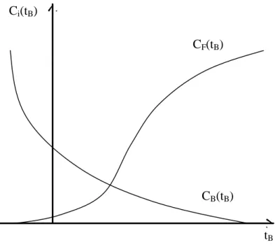
con-cave part depending on the sector’s land demand. Figure 1 depicts examples of possible contribution functions as functions of the land tax.
Ci(tB)
tB
CB(tB)
CF(tB)
Figure 1: The contribution function of sector B falls in the land tax rate tB,
but at a diminishing rate. The contribution function of sector F increases in the land tax rate tB, …rst at an increasing and then at a decreasing rate. In
the …gure we have assumed that the sector’s land use increases su¢ ciently as tB increases for the breaking point to be included in the …gure.
The marginal contribution from the biofuels sector B falls the higher the land tax rate that the government sets, a subsidy or a low tax rate thus eliciting the highest contribution from this sector. The contribution function from the forestry sector is more complicated as it depends on the sector’s land demand. A higher land tax tB, however, increases the sector’s land
the contribution function.20 At this level of generality it is impossible to say,
however, how a given level of land tax impacts the forestry sector’s mar-ginal contribution, as we have not de…ned the sector’s level of land demand, and how a given (marginal) increase in the tax impacts on the sector’s land demand. This hinges on the sector’s elasticity of land demand, which is a question to which we turn next, by making the following proposition
Proposition 3 The sector with a less elastic land demand, adjusted for the land tax rate for the biofuels sector, gives the greater marginal contribution. Proof. Examining which sector gives a higher marginal contribution in absolute terms, i.e., whether dCB0
dt0 B ? dC0 F dt0 B we …nd 1+t0 B "B T ; z ? 1 "F T ; z. In other
words, if land demand by sector B, adjusted for the land tax rate, is less elastic than land demand by sector F ( "
B T ; z
(1+t0 B)
< "F
T; z), then sector B gives a
greater marginal contribution than sector F , and vice versa.
Proposition 4 The sector with a more inelastic land demand, weighted by a constant , is the more e¤ective one in lobbying and determines the direction in which the land tax deviates from the socially optimal tax.
Proof. Examining when tB ? (TzB) yields "BT; z ? "FT; z where was de…ned
in the proof of Proposition 2. Thus, a more elastic land demand in the biofuels sector than the by weighted elasticity of land demand in forestry implies a land tax that is higher than would be socially optimal. A more inelastic land demand by the biofuels sector than the by weighted elasticity of land demand in forestry implies a land tax that is lower than would be socially optimal.
What is the economic rationale behind this? An inelastic land demand in the biofuels sector means that the deadweight loss from the tax is small. Thus, the government can "support" the sector by lowering the land tax with-out incurring a large deadweight loss, i.e., at a low cost to itself. Similarly, as the land tax on biofuels is essentially a "subsidy" to land use in forestry, the more inelastic the land demand in the forestry sector is, the lower the cost to the government for providing them with this "subsidy", i.e., the lower the deadweight loss from the subsidy (for a similar result, see, e.g., Grossman and Helpman (1994) or Dixit (1996)). Besides, in the lobbying game the sec-tor with the more inelastic land demand provides the government with the greatest marginal contribution. Consequently it "wins" as it is the one that the government can "support" at the greatest marginal bene…t and lowest cost to itself. Even the sector with the more elastic land demand can, how-ever, still have an incentive to contribute as its contribution cancels some of the e¤ect from the "stronger" sector’s contribution. This incentive falls as a sector’s land demand becomes more elastic, as the contribution has less net e¤ect.
We continue by examining how the land tax rate impacts on the elasticity of land demand. For this purpose we di¤erentiate the elasticities of land demand by the land tax to obtain:
@"B T; z @t0 B = " B T; z (1 + t0 B) " 1 + " B T; z (1 + t0 B) 1 + "B T; z "z; tB t0 B # ? 0 (13a)
@"FT; z @t0 B = " F T; z 1 + " F T; z "z; tB tB < 0; (13b) where "z; tB = @z @tB tB
z > 0 is the elasticity of land value to the land tax. An
increase in the land tax thus lowers the land demand elasticity in forestry by Equation (13b). The e¤ect arises partly directly from a change in the cost of land and partly indirectly from the change in land demand by the forestry sector, which is due to the fall in the cost of land to that sector. Both e¤ects work in the same direction.
The change in the elasticity of land demand in biofuels is, however, of ambiguous sign in Equation (13a), consisting partly of the land value e¤ect (the same e¤ect that lowers the land demand elasticity in forestry), but also of the land tax e¤ect, which serves to raise the elasticity. However, since we know that the cost of land to the biofuels sector increases in the land tax (@zB
@tB > 0 by Equation (7)), we di¤erentiate the elasticity of land demand in
biofuels by zBto obtain @"B T ; z @z0 B = " B T ; z(1+" B T ; z) z0 B > 0. Consequently we conclude
that the elasticity of land demand in biofuels increases in the land tax. In order to summarise, we formulate the following proposition:
Proposition 5 The politically optimal land tax rate serves to lower the elas-ticity of land demand by the sector whose land demand to begin with was lower, and to increase the other sector’s elasticity of land demand. Thus, the tax rate is self-enhancing.
Proof. The sector whose elasticity of land demand to begin with is lower determines the deviation in the land tax by Proposition 4. If this sector is the forestry sector, the tax rate deviates upwards, and by Equation (13a)
serves to raise the elasticity of land demand in biofuels and by Equation (13b) lowers the elasticity of land demand in forestry. The discrepancy between the elasticities increases. In a similar manner, if the biofuels sector’s elasticity of land demand to begin with is lower, the tax deviates downwards. The biofuels sector’s elasticity of land demand falls with the introduction of the tax, and the forestry sector’s elasticity increases. Again, the discrepancy between the elasticities grows. Consequently, the tax is "self-enhancing".
Proposition 5 implies that the sector that from the beginning loses con-tinues to lose in the tax-setting game. It can be compared to the result in Dixit (1996), where the marginal incentive to lobby for a further increase in price rises as the price rises. Unlike in Dixit’s model, where the sectors’ pro…ts and incentives are independent of each other except for the revenue motive, here one sector clearly loses while the other one wins, however.
We end by constructing the following thought experiment: In the "be-ginning", a forestry sector is the more productive of the two and uses most land.21 Thus, it produces at the point where the value of its marginal product
of land equals the value of land. If the government introduces some exoge-nous policy to support the use of biofuels, alternatively, if the world-market price of biofuels increases exogenously, the value of the marginal product of biofuels production increases.22 Its land demand increases, and the value
of land increases.23 Since we have assumed linear land demand in zi, the
elasticity of land demand in forestry (ceteris paribus) increases as its land demand falls, and the elasticity of land demand in biofuels falls as its land demand increases.
that supports the production of biofuels, but which attempts to internalise the external e¤ects that arise from biofuels production relative to the forestry sector by introducing a land tax, can have created a self-enhancing policy instrument that leads to a sub-optimal allocation of land to either sector. If, at the time at which the land tax is introduced, land allocation towards biofuels has taken the sectors to the point where land demand by biofuels is less elastic than that in forestry, the tax will be set at a sub-optimal level because of lobbying by the biofuels sector. This lowers the elasticity of land demand in biofuels further, and increases that in forestry, thus increasing the gap in the "lobbying e¢ ciency" of the two sectors. As the cost of setting a low tax on biofuels falls from the government point of view, the tax rate can fall further, thus creating a self-enhancing system.
Naturally, the converse also applies. Thus, if the land tax is introduced when the elasticity of land demand in forestry is still less elastic than that in biofuels, the land tax will be set at a higher than optimal level. The elasticity of land demand in forestry becomes even less elastic whereas the elasticity of land demand in biofuels becomes more elastic, and the cost for the government for increasing the tax falls. This e¤ect would counter some of the (exogenous) support given to biofuels by the government, thus raising the cost of achieving, for instance, some biofuels mandate.
5
Technological change
In this section we analyze the e¤ect of technological change in the biofuels sector. Technological change is assumed to be exogenous. As was noted
in Section 2, we assume land-augmenting technology (Romer, 2001, 9), and denote it with a technology parameter HB, so that technology enters the
pro-duction function as a multiplicator to land demand: yB(HBTB). We assume
that technological change a¤ects the external e¤ect arising from biofuels pro-duction only so far as it increases land demand by the biofuels sector.
From Equation (6), using the envelope theorem, we …nd the derivative of the land value function with respect to HB:
@z @HB = TB3 (1 + tB) TB2+ TF 2 0; (14) where @TB
@HB TB3 0 (see Appendix C) is the partial of the land demand
function in agriculture to the technology parameter. We can use this and Equation (6) to state the e¤ect of technological change in biofuels on land allocation:
Lemma 6 Technological change in biofuels increases the biofuel sector’s de-mand for land. The forestry sector’s land demand falls in technological change in biofuels.
Proof. Total land use in the model is constant, so that dTB
dHB + dTF dHB = 0. Since dTF dHB = TF 2 @z
@HB < 0 by downward sloping land demand functions and
Equation (14), then it must be that dTB
dHB = (1 + tB) TB2
@z
@HB + TB3 > 0. We
show in Appendix C that @TB
@HB TB3 > 0.
In order to determine the e¤ect of technological change on the two sectors’ welfare and on general welfare, we must de…ne the cross-di¤erentials of land demand to technology. Ti23 = @
2T i
either sector. Ti23 > 0 then implies that land demand falls slower (the land
demand function becomes ‡atter) when technology in sector B improves, whereas Ti23< 0would imply that the land demand function became steeper.
Assuming that the e¤ect is small (and since it equals zero for instance for the land demand functions used in Appendix B), for simplicity we set Ti23 = 0.
We can then solve for the cross-derivative of land value to the land tax and technology to obtain @2z @tB@HB = TB2TB3 [(1 + tB) TB2+ TF 2] 2 < 0: (15)
Starting our examination from the e¤ect that technological change has on welfare, we di¤erentiate the lobby groups’ welfare functions, given by Equation (3), and the general welfare function (Equation (5)) with respect to HB to obtain @WB(tB; z) @HB = pByB1 (1 + tB) @z @HB TB 0 (16a) @WF(tB; z) @HB = @z @HB TF < 0 (16b) @W (tB; z) @HB = pByB1TB+ z tB 0(T B) z dTB dHB (16c) From Equation (16a) we see that the welfare in the biofuels sector in-creases as technology HB increases given that the change in the value of the
marginal product of land, pByB1 exceeds the added cost to the sector from
the change in the value of land (which increases). We assume this to be the case; were it not so, the sector could choose to continue producing with its
old technology and would not be worse o¤ than before.
The forestry sector, however, only su¤ers from the increased cost of land due to the improved technology in biofuels. Thus, its welfare falls.
Finally, the change in the general welfare depends on the level of land tax, tB. If tB
0(T B)
z , i.e., if the land tax is equal to or higher than socially
optimal, then general welfare always increases when HB increases. This
depends on the improvement in the marginal product of land in sector B, when the tax rate either completely or over internalises the external e¤ect. If tB is lower than would be socially optimal, then general welfare increases
as long as tB >
0(T B)
z
pByB1TB
z(dTB=dHB). Thus, the greater the improvement in the
marginal productivity of land in biofuels (yB1), and/or the lower the change
in land demand as the technology improves (dTB=dHB), the more likely the
general welfare will improve in HB. For instance Chakravorty et al. (2009)
note that it is fully possible that a newer generation of biofuel technologies is less land intensive than the old ones, which in our framework would improve the general welfare. Nevertheless, if the land tax is set at a su¢ ciently low rate, general welfare will fall in HB because the tax does not su¢ ce to
internalise the external e¤ect.
We turn next to the contributions functions and examine how they behave as the technology in the production of biofuels improves. For the biofuels sector we di¤erentiate the marginal contribution function with respect to HB
and substitute from Equations (7), (14) and (15) to obtain @2C B(tB) @tB@HB = TF 2TB3 [(1 + tB) TB2+ TF 2]2 TB+ TF"FT; z < 0: (17a)
Since the biofuel sector’s contribution function is falling in tB, the negative
cross-derivative indicates that an increase in HB makes the sector’s
contri-bution function steeper.
The e¤ect of technological change on the forestry sector’s contribution function is ambiguous, however. Solving yields
@2C F (tB) @tB@HB = TB2TB3 [(1 + tB) TB2+ TF 2] 2TF 1 " F T; z (17b) which is positive if "F
T; z < 1, thus making the forestry sector’s contribution
function less steep, and negative otherwise. Thus, if the elasticity of land demand in forestry is low, then technological progress in biofuels serves to make the forestry sector’s contribution function ‡atter. If, however, the forestry sector has very elastic land demand ("F
T; z > 1), then its contribution
function becomes steeper in HB.
We examine the question further by di¤erentiating the land demand elas-ticities of both sectors with respect to technology, HB. Holding tB constant
we obtain @"B T; z @HB = " B T; z HB z; H 1 + "BT; z + "BT; H < 0 (18a) @"F T; z @HB = " F T; z z; H HB 1 + "FT; z > 0 (18b) where "BT; H = TB3HB
TB is the elasticity of land demand in the biofuels sector
to technology, and z; H = @H@zB
HB
z is the elasticity of the value of land to
technology. We summarise by formulating the following proposition:
Proposition 7 The biofuels sector’s elasticity of land demand falls in tech-nology and its marginal contribution increases, while the forestry sector’s
elasticity of land demand increases and its marginal contribution tends to fall. This increases the biofuel sector’s lobbying strength compared to that of the forestry sector, and leads to a fall in the land tax rate.
Proof. The proof follows from the signs of Equations (17a) and (17b) for the e¤ects on the contributions functions and from Equations (18a) and (18b) for the elasticities (assuming "F
T; z < 1). As for the e¤ect on the tax rate,
regardless of which sector has had a lower elasticity of land demand before technological change in biofuels, as the elasticity in forestry increases and the elasticity in biofuels falls, the land tax rate falls. If the land tax was initially set on a level higher than would be socially optimal, then technological change would lower it so, that it would approach social optimum or fall below it. If the land tax was initially lower than would be socially optimal, it would fall further (and could eventually become a subsidy).
It is then clear that the biofuels sector becomes "stronger" as it gets access to better technologies. The fall in its elasticity of land demand lowers the deadweight loss from giving the sector a lower tax rate. The e¤ect is reinforced by the e¤ect on the forestry sector. That sector’s land demand becomes more elastic, thus increasing the deadweight loss from the implicit subsidy to the sector.
If the land tax rate to begin with was set at a level higher than would have been socially optimal, then technological progress in the biofuels sector helps to push the economy towards the socially optimal tax rate and consequently, socially optimal land allocation. If, however, the tax rate to begin with was set "too low" or the change in lobby strength is su¢ cient to push it over
from being "too high" to being lower than would be socially optimal, then technological change leads to excessive deforestation and to a sub-optimal land allocation, where the biofuels sector uses too much land and the forestry sector too little.
6
Conclusions
In this article we have constructed a political economy model based on Gross-man and HelpGross-man (1994) to study the implementation of a hypothetical land tax on the biofuels sector, where that sector causes a negative external e¤ect compared to a forestry sector, with which it competes of land. We have shown that when two lobbies compete for a common factor of production, the supply of which is …xed but where its allocation between the sectors is variable, the existence of lobby groups representing both sectors is not enough to ensure a socially optimal outcome from the lobbying game. Instead, according to a modi…ed Ramsay rule, the sector which the government can "subsidise" in a less distorting way decideds the direction in which the land tax rate deviates from the socially optimal land tax rate. Thus, from a social optimum point of view the land tax becomes a subsidy either for land use in biofuels or in forestry, depending on which sector has the lower deadweight loss from the subsidy. The other sector’s lobbying serves to lessen the e¤ect from the …rst sector’s lobbying, however, so that the net subsidy is lower than it would be in the absence of the competing lobby group.
Furthermore, we show that the tax rate is self-enhancing. Thus, the deadweight loss of a subsidy falls for the sector which to begin with had a
lower deadweight loss from the subsidy, and it rises for the other sector, as the land tax is set to its politically optimal level. This would make it pro…table for the government to adjust the land tax rate further in the direction ben…cial to the sector with the lower deadweight loss. This question has not been pursued further, however.
We have also considered how technological change in the biofuels sector impacts on the two sectors’lobbying strength. Thus, we …nd that the elas-ticity of land demand in the biofuels sector falls in technology, while the elasticity rises for the forestry sector. This e¤ect lowers the deadweight loss from subsidising the biofuels sector and increases the deadweight loss for subsidsing the forestry sector. This can either take the economy closer to a socially optimal tax rate, if the tax to begin with was set at a level too high, or further away from the optimum, if the tax rate to begin with was ine¢ ciently low.
The introduction of di¤erent support policies for biofuels has been stud-ied, among others, by de Gorter and Just (2009b) and by de Gorter and Just (2009a). They show, among other things, that a biofuel consumer tax exemption is partly redundant, and how the introduction of tax credits for biofuels, in the presence of a biofuels mandate, ends up subsidizing fuel con-sumption instead of biofuels. The present paper complements the literature on biofuels by showing how political economy considerations, when setting biofuel policies, can lead to self-enhancing circles of adjustment, which can lead to unwanted side e¤ects, such as deforestation. On the other hand, it also shows how lobbying in some circumstances could dwarf attempts to promote the production of biofuels.
As for the other related literature, without including resource dynamics, we can explain an e¤ect similar to that in Barbier et al. (2005), namely that the relative share of land use by a non-forestry sector can be higher when the government is susceptible to lobbying. Unlike Barbier, Damania and Léonard, however, our model allows even for the opposite e¤ect where a forestry lobby can dwarf the attempts to support a non-forestry sector’s production.
We have further shown how technological progress in the non-forestry sector a¤ects the forestry sector. Our model completes that by Ehui and Hertel (1989), who show that the steady-state forest stock falls in techno-logical progress in agriculture, by including a political economy mechanism through which the e¤ect can work and be reinforced.
Finally, we o¤er a plausible explanation to the rarity of land taxation in the real world, which (to our knowledge) is lacking from the existing litera-ture. Our setting di¤ers, however, from the rest of the land tax literature in that instead of a public economics motive to land taxation, we have an envi-ronmental motive. Constructing a model of lobbying in a public economics setting is left for future research.
Notes
1Production of biogas from various wastes does not require land to grow the raw
ma-terials for biogas production. In this paper we consider those biofuels that are grown speci…cally for biofuel use, for instance, sugar cane, sugar beet, palm oil, corn or reed canary grass.
accessed on June 12th, 2009), Malaysia and Indonesia dominate the global market for palm oil, accounting for almost 90% of all exports. Between 1990 and 2005, these countries in-creased the area of palm oil plantations by nearly 5 million hectares, half of which replaced natural forests. See also Yacobucci and Schnepf (2007).
3Another oft-used policy instrument to in‡uence land use is zoning. We deem zoining
not to be a relevant policy instrument to determine land allocation between biofuels pro-duction and forestry. For the determination of zoining versus taxes we refer the reader to Netzer (2003), which is a volume investigating the impact of various tax mechanisms on regulating land use, or to Pogodzinski and Sass (1994) for a political theory of zoning.
4E.g., van der Laak et al. (2007), de Gorter and Just (2009b) and de Gorter and Just
(2009a).
5E.g., Petersen (2008), Soimakallio et al. (2009) and Yang et al. (2009). 6E.g., Pimentel et al. (2009) and Chakravorty et al. (2009).
7The case for taxing land in order to spur economic growth is strong. For instance,
George (1882), Feldstein (1977), Calvo et al. (1979) and Eaton (1988) all argue in its favor, mainly because land taxation is seen to encourage capital formation and therefore, to bene…t economic growth.
8See, e.g., Fredriksson (1997), Fredriksson (1999), Aidt (1998), Schleich (1999), Schleich
and Orden (2000), Eliste and Fredriksson (2002), Conconi (2003) and McAusland (2005).
9Of the previous studies examining the political economy of environmental policy the
one that is closest to this one is by Aidt (1998). Aidt includes three factors of production: labor, sector-speci…c capital and raw materials (e.g., oil or environmental goods such as clean water). The use of raw materials causes an externality and the imposition of an environmental tax changes the use of these. There is, however, no competition for the raw materials in Aidt’s model, and consequently, no price changes.
10A common feature of all the other political economy models based on Grossman and
Helpman is that they assume that the (industrial) lobbies organize around a …xed sector-speci…c input factor, the quantity of which does not vary in the policy instrument studied.
11H
i is assumed to be exogenous since, as we study a small open economy, the country
12The "technology" or the "e¤ectiveness of land use" parameter H
i used here is of the
same form as that used in the Solow growth model. We thus refer to HiTi as e¤ective
land use. See, e.g., (Romer, 2001, 9).
13The political economy models often assume that besides for normative reasons, such
as the internalization of externalities, taxes are also raised in order to in‡uence the income distribution (see, e.g., Grossman and Helpman (1994)), which provides a reason for the government to need to raise tax revenue. The argument cannot reasonably be used here, however, since farmers (who usually are the ones growing biofuels) most often are rather in the receiving end of income transfers. Therefore, the only justi…cation for a land tax on land under biofuels production here is the negative externality arising from land use for biofuels. Alternatively we could argue for some non-modeled government sector of the economy needing tax revenue.
14The lower restriction arises from an assumption that the cost of land for the biofuels
sector is always positive. Otherwise tB belongs to some set T, the set of possible land
taxes from which the government may choose.
15For simplicity we assume that those owning land in both uses,
BF, belong to both
lobby groups. Their net lobbying depends thus on the relative strength of respective lobby group.
16As we only assume technological change in the biofuels sector we supress the technology
term HF on forestry.
17In Feldstein’s model it is either land taxes inducing capital accumulation that raise
the rent on land, or a portfolio-balance e¤ect where individual port…lios di¤er because of di¤erences in risk perception or risk aversion, which raise the rent on land.
18It is further easy to verify that 1 dz=dtB
z < 0 given that tB
TF 2
TB2, where the
RHS is negative.
19For the same result within the framework of the Grossman and Helpman model, see,
e.g., Fredriksson (1997), Aidt (1998), Fredriksson (1999) or Schleich (1999).
20In Appendix B, using very simpli…ed speci…ed land demand functions, we …nd the
breaking point to be TF = 13. I.e., at TF < 13, the forestry sector’s contribution function
21It can be thought that in a traditional industrialised country where the energy system
has mainly been based on coal, oil, gas, hydropower and nuclear electricity, demand for biofuels has been low. Then it is feasible that the value of forestry products, as imputs for instance to a paper and pulp industry or as construction materials has greatly exceeded the value of biofuels production.
22Motives for policies that support the use of biofuels were discussed in the Introduction. 23At this point, it could be argued that even the externalities that the biofuels
produc-tion causes increase, and that the government decides to impose a land tax on biofuels production. Whether such a tax would direct the investment in biofuels towards less land intensive biofuels, or have some other economic e¤ects in the presence of the other sup-porting policies is not analysed here. For an analysis of the interaction of several policies supporting biofuels production the reader is referred to, for instance, de Gorter and Just (2009b) or de Gorter and Just (2009a).
A
Appendix
The maximization problem requires that the equilibrium characterization function (equation (9)) has a negative second order condition for a maximum. The biofuel lobby’s welfare functions is convex, however, their welfare thus reaching some minimum at some tax rate. Thus, we have
@2W B(tB; z) @t2 B = 2 @z @tB + (1 + tB) @2z @t2 B TB z + (1 + tB) @z @tB 2 TB2 = zTB2TF 2[2TB zTF 2] [(1 + tB) TB2+ TF 2]2 > 0 (19)
where we have substituted in the …rst order derivative of the value of land to the land tax from Equation (7) and the second order derivative from Equation
(8).
The forestry lobby’s welfare function is of indeterminite sign:
@2W F (tB; z) @t2 B = " @2z @t2 B TF + @z @tB 2 TF 2 # = zT 2 B2[2TF + zTF 2] [(1 + tB) TB2+ TF 2]2 (20)
where even here we have substituted in Equations (7) and (8). Even equa-tion (20) is positive if the second order derivative of land value to land tax, @2z=@t2
B is su¢ ciently small or zero. This is the case if TF < zT2F 2, i.e., at a
su¢ ciently low level of land demand by the forestry sector. If land demand by forestry is higher than zTF 2
2 , then its welfare function is concave.
What is the economic rationale behind the ambiguous second order con-dition of the forestry sector’s welfare function as given by Equation (20)? In equation (10) the second term represents the marginal welfare of the forestry sector, which is an increasing function of the land tax tB. The case where
the function is concave is straightforward: when z (tB) is su¢ ciently convex,
a small increase in the land tax induces a large fall in the value of land (cost of land to the forestry sector). This in turn leads to a large increase in the marginal welfare of the forestry sector. As the land tax increases, it induces a lesser fall in the value of land, and also the marginal welfare gain to the forestry sector becomes smaller.
If, however, the land value function z (tB) is (approximately) linear, an
regardless of the level of the tax. In this case the forestry sector’s welfare function is convex. Then, a low tax increases forestry sector’s marginal wel-fare but less than a high tax: the e¤ect from the tax on the value of land becomes cumulative and so does the e¤ect on the forestry sector’s welfare, which increases exponentially the higher the tax.
The forestry sector’s welfare function is thus S-shaped in TF. At low levels
of land demand by the forestry sector (and when the value of land function is approximatively linear), the land tax does not matter much to the marginal welfare of the sector. As the tax rate grows, the sector’s welfare grows expo-nentially. If the cost of land to forestry falls enough (is low enough) for it to reach and exceed the point where land demand TF zT2F 2, then the welfare
function reaches the portion where it is concave and the e¤ect of further tax increases gradually leads to lesser marginal increases in the sector’s welfare. At this point, the land value function z (tB) is strictly convex.
The general welfare function has the following s.o.c., where we have al-ready substituted in Equations (7) and (8):
@2W (tB; z) @t2 B = zTB2TF 2 n (TB2+ TF 2) z 00(TB) zTB2TF 2 2z h tB 0(T B) z i TB2 o [(1 + tB) TB2+ TF 2]2 (21) The multiplier in front of the "wavy" brackets is positive, and the denomi-nator is also positive. The …rst and the second terms in the wavy brackets are negative, and the third term is of indeterminate sign. If the tax rate is set at the socially optimal level, it is clear, however, that this term is equal to zero (in the social optimum tso
B =
0(T B)
z ). If the tax rate t 0
would be socially optimal (t0B <
0(TB)
z ), then the whole term is negative and
the s.o.c. of the welfare function is unambiguously negative, the function thus reaching a maximum. If, however, the tax rate is higher than would be socially optimal (t0
B >
0(T B)
z ), then the third term is positive, thus creating
an ambiguity to the sign of equation (21).
What is the economic rationale behind this? Marginal general welfare is given by the last term in equation (10). Marginal general welfare is positive, i.e., welfare grows in tB as long as tB
0(TB)
z , i.e., as long as the tax rate is
lower than would be socially optimal. At this portion of the welfare function the s.o.c. in (21) is unambiguously negative, and the welfare function reaches a local maximum at tB =
0(T B)
z . General welfare falls in tB when tB >
0(T B)
z ,
i.e., when the tax rate is higher than would be socially optimal. If tB grew
su¢ ciently for the last term in equation (21) to overweigh the two …rst ones, then the welfare function would turn convex. We consider such high land tax rates to be improbable and do not consider them further.
B
Appendix
In this appendix we derive the land tax equation and its properties using speci…ed functional forms for land demand by respective sector and the ex-ternality equation.
Land demand in biofuels is given by TB = HB (1 + tB) z, and land
demand in forestry by TF = HF z, where we will normalize HF = 1
yielding TF = 1 z. The negative net externality from land use for biofuels
The …rst order derivatives of the land demand functions are given by TB2 = TF 2 = 1. Solving further for the value of land from TB + TF = 1
yields z = HB
2+tB. This has the …rst order derivative
@z @tB =
HB
(2+tB)2 < 0 and
the second order derivative @t@22z B
= 2HB
(2+tB)3 > 0.
Substituting the land value function into the land demand functions yields land demand by biofuels, TB = 2+tHBB, and by forestry, TF =
(2+tB) HB
2+tB . Thus,
at a su¢ ciently high level of technology in biofuels, i.e., if HB 2 + tB, land
demand by forestry is zero. Substituting these into equation (10) yields
IB HB 2 + tB HB 2 + tB (1 + tB) HB (2 + tB) 2 + IF (2 + tB) HB 2 + tB HB (2 + tB) 2 a tB HB 2 + tB b HB 2 + tB HB 2 + tB (1 + tB) HB (2 + tB) 2 = 0: (22)
The elasticities of land demand in equation (11) are given by "B
T; z = 1
and "F T; z =
HB
(2+tB) HB. Examining property 3 in Proposition 2, we note that
"BT; z = "FT; z only if HB = 2+t2+bB. This is the case when land demand by
biofuels TB = 2+b1 and land demand by forestry TF = 1+b2+b, which we consider
to be a special case. Thus, at most levels of technology in biofuels, the strengths of the two lobby groups di¤er from one another.
Simplifying (22) yields tB = HB aHB IF IB+ IF (2 HB) HB + ab : (23)
In the social optimum we have tB = b.
Examining further the second order conditions of the welfare functions it is easy to show that
@2W B(tB; z) @t2 B = 3H 2 B (2 + tB) 4 > 0 (24a) @2W F(tB; z) @t2 B = HB[3HB 2 (2 + tB)] (2 + tB)4 (24b) @2W (t B; z) @t2 B = H 2 B(2tB 3b 2) (2 + tB)4 (24c) As was shown in Appendix A, the biofuels sector’s welfare function is unambiguously convex. The forestry sector’s welfare function is S-shaped; the s.o.c. is positive if HB > 23(2 + tB)and negative otherwise. Substituting
in HB = 23(2 + tB) into the equation for TF yields TF = 13. Thus, if the
share of land in forestry is less than 13, then the sector’s welfare function has a positive s.o.c. and it is convex, and if its share of land is greater than
1
3, then the welfare function is concave. Finally, the s.o.c. of the general
welfare function is negative (the function reaches a maximum at tB = b) if
tB < 32b + 1, which is the case at tB = b. Assuming tB never reaches such
a high level, we do not analyse of the portion of the function which has a positive s.o.c further.
We end by examining when land use in biofuels production could be subsidized instead of taxed (i.e., when tB is negative). Rearranging yields
IB >
IF(2 HB)
HB
+ ab
Three cases arise. If IB = 0, i.e., the biofuels lobby does not organize, it is
but IF = 0, i.e., the forestry lobby does not organize, it is su¢ cient that
b < 1a for tB to be a subsidy. The lower a, i.e., the more susceptible the
government is to lobbying, the easier it is for the biofuels lobby to get a subsidy given b. As a ! 1, the RHS becomes arbitrarily small and even for low levels of marginal externalities, land use in biofuels will be taxed. Finally, if both lobby groups organize (IB = IF = 1), land use in biofuels can
be subsidised if b < IF(2 HB)
aHB .
IF(2 HB)
aHB >
1
a, i.e., it is easier for the biofuels
sector to obtain a subsidy in the presence of the forestry lobby if HB > 2,
which in turn implies that land demand by forestry is very low (land demand by the forestry sector occurs only because of the land tax; would land use by biofuels be subsidized in this case, land demand by forestry would be zero). Thus, given positive land demand by the forestry sector, the presence of its lobby group makes it less likely that the biofuels sector gets a subsidy for its land use than would be the case in its absence.
C
Appendix
In this appendix we prove the sign taken by the …rst order derivative of the land demand function for sector i with respect to Hi. We start by solving
for the marginal product of land as
yiT = pj(1 + ti) Hj pi(1 + tj) Hi
yTj. (25)
dyi T dHi = yiT T @Ti @Hi + @Ti @zi @zi @Hi + yT Li @Li @Hi + @Li @zi @zi @Hi = pj(1 + ti) Hj pi(1 + tj) Hi 1 pjHj @zj @Hi yjT Hi ! : (26)
Substituting in the …rst order condition of the marginal product of the la-bor -function with respect to Hi:
dyi L dHi = y i LT @Ti @Hi + @Ti @zi @zi @Hi +y i LL @Li @Hi + @Li @zi @zi @Hi = 0 and @zj @Hi = (1 + tj) @z
@Hi and simplifying yields
Ti3= @Ti @Hi = y i LLyTi Hi i ; (27) where yi
T > 0 is the marginal productivity of land. Since we assume that
the production function yi is increasing in Ti and Li but at a falling rate, we
have yi
T T < 0 and yiLL < 0. i = yT Ti yiLL (yiT L) 2
> 0. This completes the proof.
References
Aidt, T. S. (1998). Political internalization of economic externalities and environmental policy. Journal of Public Economics 69, 1–16.
Barbier, E. B., R. Damania, and D. Léonard (2005). Corruption, trade and resource conversion. Journal of Environmental Economics and Manage-ment 50, 276–299.
allo-cation, and economic in‡uence. Quarterly Journal of Economics 101 (1), 1–32.
Calvo, G. A., L. J. Kotliko¤, and C. A. Rodriguez (1979). The incidence of a tax on pure rent: A new (?) reason for an old answer. Journal of Political Economy 87 (4), 869–874.
Chakravorty, U., M.-H. Hubert, and L. Noestbakken (2009, April). Fuel versus food. Technical report, Department of Economics, University of Alberta.
Conconi, P. (2003). Green lobbies and transboundary pollution in large open economies. Journal of International Economics 59 (2), 399–422.
de Gorter, H. and D. R. Just (2009a). The economics of a blend mandate for biofuels. American Journal of Agricultural Economics 91 (3), 738–750. de Gorter, H. and D. R. Just (2009b). The welfare economics of a biofuel tax credit and the interaction e¤ects with price contingent farm subsidies. American Journal of Agricultural Economics 91 (2), 477–488.
Dixit, A. (1996). Special-interest lobbying and endogenous commodity tax-ation. Eastern Economic Journal 22 (4), 375–388.
Eaton, J. (1988). Foreign-owned land. American Economic Review 78 (1), 76–88.
Ehui, S. K. and T. W. Hertel (1989). Deforestation and agricultural pro-ductivity in the cÃtte d’ivoire. American Journal of Agricultural Eco-, nomics 71 (3), 703–711.
Ehui, S. K., T. W. Hertel, and P. V. Preckel (1990). Forest resource depletion, soil dynamics, and agricultural productivity in the tropics. Journal of Environmental Economics and Management 18 (2), 136–154.
Eliste, P. and P. G. Fredriksson (2002). Environmental regulations, transfers, and trade: Theory and evidence. Journal of Environmental Economics and Management 43 (2), 234–250.
Feldstein, M. (1977). The surprising incidence of a tax on pure rent: A new answer to an old question. Journal of Political Economy 85 (2), 349–360. Fredriksson, P. G. (1997). The political economy of pollution taxes in a
small open economy. Journal of Environmental Economics and Manage-ment 33 (1), 44–58.
Fredriksson, P. G. (1999). The political economy of trade liberalization and environmental policy. Southern Economic Journal 65 (3), 513–525.
George, H. (1882). Progress and poverty : an inquiry into the cause of indus-trial depressions and of increase of want with increase of wealth. London: Kegan Paul, Trench and Co.
Goldberg, P. K. and G. Maggi (1999). Protection for sale: An empirical investigation. American Economic Review 89 (5), 1135–1155.
Grossman, G. M. and E. Helpman (1994). Protection for sale. American Economic Review 84 (4), 833–850.
Hyytiäinen, K., J. Leppänen, and T. Pahkasalo (2008). Economic analysis of …eld a¤oresttion and forest clearance for cultivation in …nland.
Tech-nical report, 12th Congress of the European Association of Agricultural Economists.
Lankoski, J. and M. Ollikainen (2008). Bioenergy crop production and cli-mate policies: a von thunen model and the case of reed canary grass in …nland. European Review of Agricultural Economics 35 (4), 519–546. Le Breton, M. and F. Salanie (2003). Lobbying under political uncertainty.
Journal of Public Economics 87 (12), 2589–2610.
Lindholm, R. W. (1979). Public choice and land tax fairness. American Journal of Economics and Sociology 38 (4), 349–356.
Magee, C. (2002). Endogenous trade policy and lobby formation: An applica-tion to the free-rider problem. Journal of Internaapplica-tional Economics 57 (2), 449–471.
McAusland, C. (2005). Harmonizing tailpipe policy in symmetric countries: Improve the environment, improve welfare? Journal of Environmental Economics and Management 50 (2), 229–251.
Mitra, D. (1999). Endogenous lobby formation and endogenous protection: A long-run model of trade policy determination. American Economic Re-view 89 (5), 1116–1134.
Netzer, D. (Ed.) (2003). The Property Tax, Land Use and Land Use Regu-lation. Cheltenham, U.K. and Northampton, Mass.: Elgar in association with the Lincoln Institute of Land Policy.
Olson, M. (1965). The Logic of Collective Action: Public Goods and the Theory of Groups. Cambridge, Mass.: Harvard University Press.
Petersen, J.-E. (2008). Energy production with agricultural biomass: En-vironmental implications and analytical challenges. European Review of Agricultural Economics 35 (3), 385–408.
Pimentel, D., A. Merklein, M. A. Toth, M. N. Karpo¤, G. S. Paul, R. Mc-Cormack, J. Kyriazis, and T. Krueger (2009). Food versus biofuels: Envi-ronmental and economic costs. Human Ecology 37, 1–12.
Pogodzinski, J. and T. R. Sass (1994). The theory and estimation fo endoge-nous zoning. Regional Science and Urban Economics 24 (5), 601–630. Ricardo, D. (1817). On the Principles of Political Economy and Taxation.
Kitchener, Ontario, Canada: Batoche Books.
Romer, D. (2001). Advanced Macroeconomics (2nd edition ed.). Boston: McGraw Hill.
Schleich, J. (1999). Environmental quality with endogenous domestic and trade policies. European Journal of Political Economy 15 (1), 53–71. Schleich, J. and D. Orden (2000). Environmental quality and industry
protec-tion with noncooperative versus cooperative domestic and trade policies. Review of International Economics 8 (4), 681â ¼A¸S697.
Soimakallio, S., T. Mäkinen, T. Ekholm, K. Pahkala, H. Mikkola, and T. Pap-panen (2009). Greenhouse gas balances of transportation biofuels,
electric-ity and heat generation in …nland - dealing with the uncertainties. Energy Policy 37, 80–90.
van der Laak, W. W. M. v. d., R. P. J. M. Raven, and G. P. J. Verbong (2007). Strategic niche management for biofuels: Analysing past experiments for developing new biofuel policies. Energy Policy 35, 3213–3225.
WWF (2008). Wwf position paper on bioenergy.
WWF (2009). Oil palm, soy and tropical forests: a strategy for life.
Yacobucci, B. D. and R. Schnepf (2007). Ethanol and biofuels: Agriculture, infrastructure, and market constrints related to expanded production. En-ergy Bulletin.
Yang, H., Y. Zhou, and J. Liu (2009). Land and water requirements of biofuel and implications for food supply and the environment in china. Energy Policy 37, 1876–1885.