A acroSpeedFlowModel
for Multllane Roads
Reprint from Proceedings of the Third International
Symposwm on Highway Capacity, Copenhagen i
*
Denmark June 1998
Arne Carlsson and Hans-Åke Cedersund
O'! c» m 91 m 14
oo
x 0 >» &. q.: &. NB (I)Copenhagen, Denmark, June, 1998
::;j elekekRysgaard
' iEdltor ' , i '
VM".Road Directorate gm;
moon-Denmark
Swedish National Road and
' ansport Research Institute
VTI särtryck 315 - 1999
A Macro Speed-Flow Model
for Multi-Iane Roads
Reprint from Proceedings of the Third International
Symposium on Highway Capacity, Copenhagen,
Denmark, June 1998
Arne Carlsson and Hans-Åke Cedersund
§Wedieii
and
Abstract
The National Road Administration in Sweden has initiated a comprehensive research project concerning traffic on multilane roads, called TPMA (Traffic Performance on Major Arterials). One stage of this project is to develop a macromodel for basic four-lane road segments. This model is based on traffic data from sites with different road performances and posted speed limits. Three vehicle types are analysed: car, truck and
bus, and truck with trailer.
The model comprises four submodels:
1. A submodel for the lane distribution of the numbers of vehicles as a function of the
total traffic flow and proportion of heavy vehicles.
2. A submodel for free flow speed for each vehicle type, each lane and each posted speed limit.
3. A submodel for lane capacity for each driving lane. The model has a base capacity and adjustment factors.
4. A submodel for the speed-flow relationship. The speed flow curve is partly linear in three sections.
The model states that at high traffic volumes an increasing proportion of cars use the left lane with higher speeds and capacity values for this lane. The total capacity is
3900 4500 vehicles per hour for both lanes with about 55% of the vehicles running in
the left lane. This is due to arterials with mainly inbound traffic to the city centra. For arterials with outbound traffic from the city centra the total capacity is about 500 vehicles per hour higher, i.e. 4,400-5,000 vph.
Contents
1. INTRODUCTION
2. STRUCTURE OF THE MODEL 3. DATA ACQUISITION
4. DATA PROCESSING
4.1 Data Processing For the Lane Distribution Model 4.2 Data Processing for the Other Submodels
5 LANE DISTRIBUTION MODEL 5.1 Purpose
5.2 Method
5.3 Results from the lane distribution model
6. FREE-FLOW MODEL 6.1 Purpose
6.2 Build up of the Model 6.3 Method 6.4 Results 7. CAPACITY MODEL 7.1 Purpose 7.2 Method 7.3 Results
8. SPEED-FLOW RELATION MODEL 8.1 Purpose
8.2 Method 8.3 Results
9. DISCUSSION AND SUMMARY
Page C C O O O O O O O N A A -B ä n ) ! » U) H H H v a r -M d » U I N N N b ib il ib i N I O N O N O N N ©
1. INTRODUCTION
The Swedish National Road Administration (SNRA) has commissioned the Centre for
Traffic Engineering and Traffic Simulation (CTR) to conduct a major development project designated TPMA (Traffic Performance on Maj or Arterials).
TPMA comprises the development of three models a macromodel and two micro models treating the driver/vehicle as one and two objects respectively. The models describe the traffic process on multi lane roads with traffic interchanges and will pro vide a basis for various effect calculations in the National Road Administration's project design and planning system.
Work started in spring 1996 with further development and formulation of detailed proposals for methods for the various submodels (e.g. literature studies, inventories, empirical data requirements, choice of measuring sites, data acquisition and processing, model development and analysis, etc.) During 1996 and 1997, an extensive programme of data acquisition and processing has been carried out as a basis for designing both the macromodel and micromodels.
The first stage in the macromodel entails the development of a speed flow model for four-lane arterials. This model consists in turn of four submodels indicating lane
distribution in various traffic flows, free flow speed in various road performances,
capacity per lane and speed-flow relation.
This document describes the development work and the results obtained with the
macromodel and its submodels.
2. STRUCTURE OF THE MODEL
The model developed consists in principle of four submodels with the following
structure:
1. A lane distribution model. 2. A free flow speed model. 3. A capacity model.
4. A speed-flow relation model.
The basic approach includes developing separate submodels for left and right lanes. All measurements show significant differences in behaviour between the two lanes. This applies to effects such as speed, vehicle density and proportion of heavy vehicles. Submodels 2 4 therefore have different variable values for the left and right lanes. In general, the model is intended to operate with three vehicle types as follows:
1. Car (and light truck).
2. Truck without trailer and bus. 3. Truck with trailer.
These three vehicle types normally have different speed limits. The model therefore describes speed behaviour for each vehicle type.
The four submodels are described below.
l . Lane distribution model
This submodel calculates the number of vehicles of each type for the right and left lanes respectively. Input data consist of the total traffic ow in one direction and the proportion of heavy vehicles (buses and trucks with/Without trailer). The time interval for flow and proportion of heavy vehicles is one hour.
2. Free- ow speed model
The free- ow speed is determined for each vehicle type and lane. The model is a simple additive model with a basic speed for each vehicle type and adjustment factors for:
lane width
distance to a barrier
hard shoulder Width
The base speed and adjustment factors for each lane are dependent on various speed limits.
3. Capacity model
A value for capacity is determined for each lane. The model is multiplicative with a basic value and adjustment factors for the proportion of heavy vehicles and distance to
roadside obstacles.
It should be noted that in this approach the model uses ow in vehicles per hour and the proportion of heavy vehicles per lane instead of pce.
4. Speed ow relation model
The speed ow curve (v q curve) is built up as partly linear portions in three sections.
For low and medium flows, the curve is at, but becomes steeper at degree of
3. DATA ACQUISITION
To obtain a basis for model design, field measurements in the form of spot speed mea surements were performed on many sections, primarily the heavily used arterials around Sweden's three largest cities Stockholm, Gothenburg and Malmö. During
1994, 1996 and 1997, measurements were made at about 50 sites on arterials.
Data acquisition was designed mainly according to the following principles:
Several consecutive measuring sites (up to 4 5) were chosen on the same or immediately following arterial segment in the direction of the road. Consequently, it was mostly road performance or speed limit that changed between the sections. In addition, an effort was made to perform the measurements in both directions at the same time. In each section, measurements were made so that the detectors (usually rubber tubes) covered one lane only. The traffic in each lane has thus been measured individually.
4. DATA PROCESSING
The collected data distributed per lane have been converted to a vehicle file using a
special software from The Swedish Road and Transportation Research Institute (VTI)
called PREC95, see (Anund and Sörensen 1995). This program provides information on arrival time, vehicle type, spot speed and axle distance for each individual vehicle. As a measure of quality, data were also obtained on the number of passing axles not converted to vehicles. In general, this number is about 0.2 0.5 % of all passing axles. 4.1 Data Processing For the Lane Distribution Model
For the lane model, only flows and traffic composition were analysed. Six different
measuring sites were chosen for this model. For these sites, the flow was calculated for
one hour as a total for both lanes and for the right lane alone. In addition, the number of vehicles of each vehicle type was calculated as above. The flow calculation was
made on a rolling basis with start min 00, min 05, min 10 and so on. This gave rolling
mean values with 12 observations per hour.
In this way, a large number of observations of hourly flows were obtained. The material was divided into four classes according to the proportion of heavy vehicles as
a total for both lanes. These four classes were 0 5 %, 5 10 %, 10-15 % and 15 20 %
heavy vehicles. For each measuring site, this gave four classes with observations of total hourly flow and flow in the right lane. To illustrate the result, the flow in the right lane was plotted as a function of the total flow. Each plot contains three curves the total number of vehicles in the right lane, the number of vehicles of type 1-2 in the right lane and vehicle type 1 alone.
4.2 Data Processing for the Other Submodels
To enable capacity calculations and study of speed ow (v q) relations, several speed-flow curves have been plotted for each measuring site and lane using the following method.
The measuring time has been divided into time intervals, each of which comprises 200
cars (type 1) in one lane. Consequently, the interval is not constant in time but varies with traffic flow. High flows give short time intervals and vice versa. The total number of vehicles of all three types in such an interval is counted and transformed into a hourly flow. For each vehicle type the space mean speed was calculated. This gives three speed flow curves one for cars, one for trucks and one for trucks with trailer. In addition, density for each time interval is calculated. This is done by calculating the space mean speed for all vehicles in the interval. The general relation d=q/v (density=traffic flow/speed) then applies to the calculation of vehicle density in vehicles per hour and lane. These data are used in the analysis for estimating parameters in a number of traffic models of standard character, where speed is expressed as a function of density.
5 LANE DISTRIBUTION MODEL 5.1 Purpose
The submodel for lane distribution indicates the number of vehicles of each type in each lane on an hourly level. Input data consist of the total flow for one direction and the proportion of heavy vehicles in the flow. The model can be illustrated as follows:
Total flow in both lanes, proportion of heavy vehicles
==>
Number of cars/Number of buses and trucks without trailer/ Number of trucks with trailer
in
right and left lane respectively 5.2 Method
The chosen approach for the model was:
Q. = {K * ( 1 - exp( L * Q....» %
(1)
K and L are parameters
In the model, K indicates the absolute maximum ow in the right lane (capacity in the
right lane), while L indicates the form of the curve. In large total ows, almost all
growth thus occurs in the left lane.
To estimate the model parameters K and L, data from six chosen measuring sections were used. For each 60 minute period, total flow and proportion of heavy vehicles were calculated. In addition, the number of vehicles of type 1, the number of types 1 and 2 and the number of types 1, 2 and 3 in the right lane were calculated. For each
hour, a 60 minute period starting at min 00, min 05, min 10 and so on was calculated.
This gave 12 periods for one hour of traffic.
Where possible, the observations from the 60-minute data were divided into four classes with the following proportions of heavy vehicles (types 2 and 3): 0-5 %, 5
10 %, 10-15 % and 15-20 %. Time periods with proportions of heavy vehicles exceeding 20 % and in some cases greatly exceeding this level, have been excluded. Using non linear regression, the parameters K and L were estimated for each measuring site and proportion of heavy vehicles. No clear tendencies were thereby obtained for either of these parameters.
The next step was to try to express K, which indicate the maximum ow in the right lane, partly in ideal conditions and partly with different proportions of heavy vehicles. A reasonable approach is shown below:
K= {2600[1 0.2*0Lh*oc*2.0 0.5*Bh*B*2.0]} (2) 2,600 is a theoretical maximum ow in the right lane. The value is reduced by the expression in brackets.
oc is the proportion of trucks without trailer and buses (type 2) in the total flow for both lanes,
B is the proportion of type 3 vehicles in the total ow for both lanes, 0th is the proportion of type 2 vehicles travelling in the right lane, Bh is the proportion of type 3 vehicles travelling in the right lane,
0.2 is based on an assumed pce value of 1,2 for vehicle type 2, which in turn is based
on a time headway of 1,8 sec in a queue compared with 1,5 sec for a car,
0.5 is based on an assumed pce value of 1,5 for vehicle type 3, which in turn is based
2.0 is the absolute max ow for both lanes together seen in relation to the maximum
flow in the right lane, that is 5,200 and 2,600 cars respectively.
To determine och and Bh, it is necessary to know whether these proportions vary with the total flow. The plot of the proportion of vehicles of types 2 and 3 travelling in the right lane at different sites showed a weakly negative relation (the proportion in the right lane decreased weakly with increasing total flow). However, the dispersion is very pronounced. With reasonable accuracy, it can be said that the proportions are constant. From the plots, och was determined as 0.85 and Bh as 0.90. The material also showed that the proportion of vehicles of type 2 is twice as high as the proportion of type 3. Using the above data, the following K values were used for calibration for different proportions of heavy vehicles.
Propotion of heave cehicles Calculated K-value 0 5 % (2,5) 2566
5-10% (7,5) 2497 10 15% (12,5) 2429 15 20% (17,5) 2360
In regression with fixed K values as above, more consistent L values were obtained. In addition, it was found that L increased for all sites when the proportion of heavy vehicles increased.
5.3 Results from the lane distribution model
The results of the calibration for the lane distribution model are presented in Table 1 below.
The flow in the right lane is determined by Equation (l) with K and L values as in Table ] below:
Table 1 - Calibrated values of K and L at different proportions of heavy vehicles. Proportion of heavy vehicles K-value L value
0-5 % 2566 0.00032 5 10% 2497 0.00034 10 15% 2429 0.00036 15-20% 2360 0.00038
The table values above refer to the proportion of heavy vehicles in the middle of the
If exact values for oc and B are obtained, L is calculated according to the expression:
L= {(3.1+4*(0c+[3))*104}
M3)
oc and B are the proportion of vehicles type 2 and 3 in the total flow. In the same way, the K value is calculated according to the Equation (Z):
With och = 0.85 and [3h = 0.90, we obtain:
K = {2600 [1 - 0.34 m - 0.90 * B] }
(4)
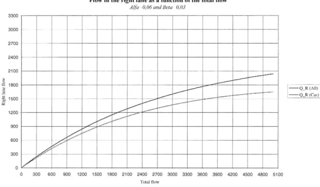
Figure ] below shows how the flow in the right lane depends on the total flow for both lanes. The relationsship applies to a proportion of heavy vehicles of 9 % as above, 6 % for type 2 and 3 % for type 3. The upper curve shows the total number of vehicles in the right lane and the lower curve the number of cars.
Flow in the right lane as a function of the total ow
AlfazO, 06 and BetazO, 03 3300 3000 2700 2400 2100 & 1800 /// __? 2 / l - -Q_R (All) : ; 1500 / M...Mww'ww'wwww hi! 3953 EJ //*M M""...-1200 //,,,w .» ."-"'" 900 if g 600 ///" / 300
%
0 300 600 900 1200 1500 1800 2100 2400 2700 3000 3300 3600 3900 4200 4500 4800 5100 TmMHow
Fig. 1 - Flow in the right lane as a function of the total flow
As shown in Figure l, the flow in the right lane is less than in the left lane at total ows greater than about 3,600 vehicles per hour. The number of cars in the right lane
follows the same curve as the total flow for this lane, but at a lower level. However, the
difference increases with increasing total flow.
Validation of the lane distribution model will be performed against data from field measurements in 1998 in the TPMA project. A slight modification has already been
done. In the first calibration a value of 2,400 was chosen for K, but this did not give values in agreement with the capacity model presented in section 7.3 below. Therefor
the K value was changed to 2,600.
6. FREE-FLOW MODEL 6.1 Purpose
The submodel for free-flow speeds must produce a free flow speed for each vehicle type (three types) and each lane. In addition, the model must contain adjustment parameters describing the in uence of various geometric designs. A set of data must be provided for each of the speed limits 70, 90 and 110 km/h.
6.2 Build up of the Model
An additive model in accordance with (HCM 1994) shall be developed with the purpose of determining free- ow speed (expressed in space mean speed) for a four lane arterial. For the left lane, the model expression is:
FVV Zäll Vw _ FL _ FK _ FHV j (5)
where
FV : free flow speed in the left lane for the particular road performance and vehicle type (one speed for each vehicle type),
FVOV = speed in ideal conditions in the left lane, FL : adjustment factor for the terrain type, FK : adjustment factor for lane width,
FHV : adjustment factor for distance to roadside obstacle (left) less than 2 metres. A distance of more than 2 metres has no in uence.
It should be observed that the model does not include the width of an inner hard shoulder, but only the distance to a possible barrier. If, for example, the inner hard shoulder is 0.5 m but there is a median without roadside obstacles, Fm, = 0.
For the right lane, the corresponding model expression is:
FVH = {FVOH " FL ' FPS _ FK _ FVR % (6)
FVH = free flow speed in the right lane for the particular road performance and vehicle type (one speed for each vehicle type),
FVOH = speed in ideal conditions in the right lane, FL: as above,
FPS = adjustment factor for cars with trailer (incl. caravans),
FK = as above,
FVR = adjustment factor for width of right hard shoulder, including occurrence of possible roadside obstacle. A hard shoulder width exceeding 3 m has no influence.
Note that in regard to the right hard shoulder, it is the width of the hard shoulder that is
included in the model. The size of the adjustment factor is not influenced by a possible barrier.
Note also that all speeds and adjustment factors above are dependent on the speed limit but not on the proportion of heavy vehicles, since the latter factor has no in uence on the free flow speed. All the above speeds and adjustment factors are determined through data analysis.
Almost all data acquisition has taken place on level arterials. Therefore there is no information for determining the factor FL. In an initial step, only the free flow model for level terrain with FL=O has been developed. At present, there is no information for other types of terrain.
6.3 Method
To determine the parameters for the free ow submodel, data from almost all measuring sites were used. For each site and lane, an estimate was made of the free-flow speed for each vehicle type. This was done by taking plotted diagrams of measured speed flow and estimating the speed in the flow interval 400 600 vehicles per hour. It was found that at flows below 400 vehicles per hour a large dispersion was obtained in the observations, due to the fact that the majority of these were recorded during night time and early morning when the speed dispersion is large. The 400 600
vehicles per hour interval has a much more stable level. At higher flows, a reduction in
speed begins to be observed.
The ideal speed and adjustment factors are estimated with linear regression. In the final table, the adjustment factors have been corrected somewhat to give consistent values.
6.4 Results
Using the results from the regression analysis, ideal speeds and adjustment factors has
been estimeted. Table 2 shows the speed in ideal conditions, which means more than
2.0 m to a roadside obstacle for the left lane and 3.0 m width of the right hard shoulder. The lane width can vary from 3.25 to 3.75 m without speed being influenced.
Table 2 - Ideal speed FV0 (km/h) for left and right lane.
Type of vehicle 110 km/h 90 km/h 70 km/h left right left right left right
lane lane lane lane lane lane
Car 116 105 106 94 85 76
Truck and bus 106 92 98 87 84 74 Truck with trailer 92 85 91,5 84,5 81 73
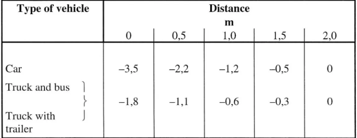
Table 3 gives the adjustment factor FHV for distance to a roadside obstacle from the edge of the left lane. The basis has been a speed difference of 3.5 km/h for a car between 0 and 2 m. However, the final relation has been made non-linear with greater
influence at small distances. In addition, the adjustment factor for heavy vehicles has
been set at half the value for a car.
Table 3 - Adjustment factor FHV (km/h) for distance to a roadside obstacle from the left lane. Speed limit 90 and 110 km/h.
Type of vehicle Distance
m
() 0,5 1,0 1,5 2,0
Car 3,5 2,2 -1,2 0,5 0
Truck and bus l
%
1,8
1,1
0,6
o,3
0
Truck with J
trailer
Note that arterials with a 70 km/h limit have no adjustment factor. Because of the limited material and irrelevant values in the regression, no adjustment factors were used for this speed limit.
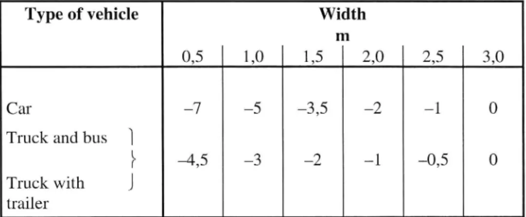
The adjustment factor for a right hard shoulder is given in Table 3. The starting point is thus a reduction of 7.0 km/h when a hard shoulder decreases from 3.0 to 0.5 m. However, just as in the above, the relation is non-linear and the speed reduction is greater for a narrow hard shoulder. The adjustment factor for heavy vehicles is less than for cars.
Table 4 - Adjustment factor FVR (km/h) for a right hard shoulder. Speed limit 90 and 110 km/h.
Type of vehicle Width
m
0,5 1,0 1,5 2,0 2,5 3,0
Car 7 5 3,5 2 1 0
Truck and bus l
%
4,5
-3
2
1
0,5
0
Truck with J
trailer
Finally, the factor FPS is calculated. This is the adjustment factor for a car with trailer. On 110 km/h roads, the speed difference between these types of vehicle is on average 21 km/h. At the ideal speed of 105 km/h, the following speed was obtained with 2% cars with trailer:
l/[0.98/105+0.02/84]:104.5 km/h. Thus, FPS was set to 0.5 km/h.
On 90 km/h roads, the following was obtained in the same way with a speed difference of 13 km/h:
1/[0.98/94+0.02/81]=93.7 km/h. Thus, FPS: -0.3 km/h.
As mentioned above, only level arterials are treated in this step and consequently no value is assigned to FL.
For the lane width factor FK it was impossible to get any relation between speed and lane width in the regression analyses. Consequently this adjustment factor was set to FK = 0 (for lane width between 3.25 and 3.75 m).
The additive model was chosen in accordance with the HCM model for multilane highways (HCM 1994). The results show that there are just one or two adjustment factors for each lane, which indicates that there is no need for a multiplicative model. Besides the variations in road performance data are small. The distance to a left roadside obstacle is normally 1 2 m and the right shoulder width is 1,5 3 m.
7. CAPACITY MODEL
7.1 Purpose
The submodel for capacity aims at analysing how capacity is influenced by road performance and the proportion of heavy vehicles. All the measuring sites were located on straight level roads, and so the original purpose of also taking the type of terrain
into account has not been dealt with here. Instead, this factor has been left to a
micromodel to analyse when this has been developed. The model for capacity per lane has been formulated in the following multiplicative expression:
Ci: {Cm * Fk * 1::hv * F1 } (7)
i : left and right lane respectively where
Ci is the capacity of the right and left lane respectively C i is the basic capacity in ideal conditions
Fk is the adjustment factor for lane width and distance to a roadside obstacle Fhv is the adjustment factor for the proportion of heavy vehicles
F1 is the adjustment factor for type of terrain. (However, F1 has been set to 1.0 for
a level road).
Note that the flow is defined in vehicles per hour and not in car equivalents. 7.2 Method
Speed ow diagrams have been drawn up for all measuring sites. Each point in the diagrams corresponds to the mean speed of 200 cars. The flow is calculated on the basis of the total number of vehicles during the corresponding time period.
The capacity has been estimated for those measuring sites where a clear speed ow dependence was observed. The most of these sites were inbound traffic towards city centre. The estimate of capacity was made in several ways. First and foremost, a visual observation of capacity was made on the basis of the above mentioned speed- ow diagrams. In addition to this, capacity was calculated with the aid of classical traffic
stream models in which the speed is described as a function of density, see (May 1990).
The following models have been used:
Generalized Single Regim V: vf>x< [1-(K/Kj)(" ] / '
Greenshield V= Vf* (l K/Kj) Underwood V= Vf * exp( K/ Km) Northwestern V: Vf * exp[ 0.5(K/Km)2]
Extended Northwestern
V: V,? exp[ (l/n)(K/Km)"]
where
V : speed, space mean speed, of cars Vf: free flow speed
K : density
K. = täthet at a jam, traffic standstill [ and n are constants,
Km : density at maximum flow.
"Extended Northwestern" has been developed as part of the project to facilitate finding a flexible V K adaptation compared to the normally bell shaped Northwestern. Using for example n=2 in "Extended Northwestern", we obtain the ordinary Northwestwern model.
The parameters in all the above models have been estimated for the right and left lane respectively on all measuring sites with high flows. This estimate has been made with non linear regression in calculated speed density data. In the final run an estimate of the parameters was made with the free flow value for each site and lane fixed at the free flow speeds used above in Section 6.3.
For twelve measuring sites, mostly with inbound traffic, there is a pronounced analysable v q dependence, which is used to estimate the parameters. The capacity can be calculated explicitly from all the traffic stream models when the model parameters have been estimated. The same applies to speed and density at the capacity limit. However, although the v-q relation is sometimes very clearly marked, the different models produce widely varying capacity values. In practice, only moderately realistic capacity values are obtained from the Generalized Single Regime (GSR) and "Extended Northwestern (NW)". The calculated residuals are approximately of the same size for both these models despite their differences in model assumptions. Other models' capacity values have been calculated but rejected.
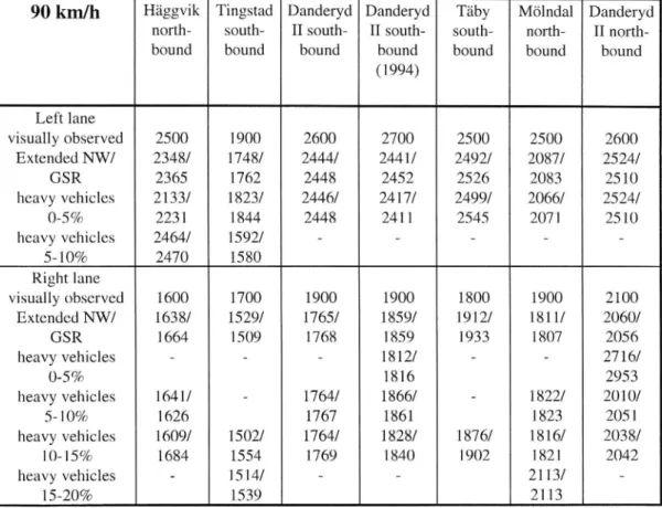
The most realistic values are obtained when the free-flow speed in the model is fixed at the estimated free flow speeds. Table 5 below illustrates the results from sites with speed limit 90 km/h.
Table S - Capacity, visually observed and calculated from two traf c stream models, for sites with speed limit 90 km/h.
90 km/h Häggvik Tingstad Danderyd Danderyd Täby Mölndal Danderyd north- south- II south- II south south north II north-bound bound bound bound bound bound bound
( 1994) Left lane visually observed 2500 1900 2600 2700 2500 2500 2600 Extended NW/ 2348/ 1748/ 2444/ 2441/ 2492/ 2087/ 2524/ GSR 2365 1762 2448 2452 2526 2083 2510 heavy vehicles 2133/ 1823/ 2446/ 2417/ 2499/ 2066/ 2524/ 0 5 % 2231 1844 2448 241 1 2545 2071 25 10 heavy vehicles 2464/ 1592/ - -5- 10% 2470 15 80 Right lane visually observed 1600 1700 1900 1900 1800 1900 2100 Extended NW/ 163 8/ 1529/ 1765/ 1859/ 1912/ 181 1/ 2060/ GSR 1664 1509 1768 1859 1933 1807 2056 heavy vehicles - 1812/ - 2716/ 0-5 % 1 816 2953 heavy vehicles 1641/ - 1764/ 1866/ 1822/ 2010/ 5 10% 1626 1767 1861 1823 2051 heavy vehicles 1609/ 1502/ 1764/ 1828/ 1876/ 1816/ 203 8/ 10-15% 1684 1554 1769 1840 1902 1821 2042 heavy vehicles - 1514/ - - 21 13/ 15 20%
1539 2113
As can be observed in the table the calculated capacity values agree fairly well with the visually observed values for the entire data material. When the material is divided up between various heavy vehicle classes, the calculated values become more uncertain. No clear trend can be distinguished from the data. For the left lane, the proportion of heavy vehicles so seldom exceeds 5% that it is not analysable.
Therefore a calculation of the relation including all the other measuring sites with high flows was made. This indicated that capacity decreases by about 2 3 % for a proportion of heavy vehicles of 5 10 % compared with 0-5 %, and by another 3 % in comparison between a proportion of 10 15 % and one of 5-10 %. On the basis of these values, an estimate of the factor Fhv is made, see following section.
The data material from sites with outbound traffic were analysed by comparing the 95 98 percentile in measured ow between the inbound and outbound sites. It is obvious that the ows for outbound traffic on the 90 km/h sites are significant higher and normally there are no Visually observed capacity.
Difficulties exist in analysing the relation between capacity and road performance, distance to roadside obstacles and lane width. The material is too limited and the capacity values too uncertain, especially when comparing with a corresponding analysis for free ow speed where it was possible to analyse almost all the material, The adjustment factor "Fk" must therefore be excluded from the model.
Owing to the high level of uncertainty, the numerical value of capacity must be specified with a large margin.
7.3 Results
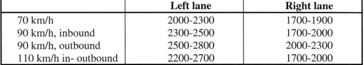
Reasonable intervals for capacity at 70, 90 and 110 km/h are shown in Table 6 below. Table 6 - Capacity at 70, 90 and 110 km/h, right and left lane respectively.
Left lane Right lane 70 km/h 2000 2300 1700 1900 90 km/h, inbound 2300 2500 1700-2000 90 km/h, outbound 2500 2800 2000 2300 110 km/h in outbound 2200-2700 1700-2000
Capacity is higher in the left lane than in the right lane. In this context very special conditions apply to a motorway section with a speed limit of 70 km/h. Because of poorer road performance and proximity to traffic interchanges combined with extreme traffic flows, the speed limit has been set as low as 70 km/h. The same applies to 90 km/h to a certain extent.
A special problem is that high ows only occur on arterials close to the largest cities. The segments between interchanges are relatively short and often have considerable flows on the ramps. The inbound sites often have a disturbing on-ramp with high flows either upstream or downstream. The outbound sites have off ramp with high ows up or downstream. In these sites a high speed level normally is maintained despite the flows are higher than those for the inbound sites. The table values must be regarded as capacity values for arterials with relatively short distances to ramps. For the 90 km/h
sites, which are located in the zone between urban and rural areas, the in uence from
an on ramp and off ramp are different. That is why different values are presented in the table.
A summary of the model s adjustment factors is given below:
see Table 6 above, different for inbound and outbound traffic
omitted
0.98 for a proportion of heavy vehicles of 0-5 % in left lane 0.99 for a proportion of heavy vehicles of 0 5% in right lane 0.96 for a proportion of heavy vehicles of 5-10 %
0.93 for a proportion of heavy vehicles of 10-15 % 0.90 for a proportion of heavy vehicles of 15-20 %
8. SPEED-FLOW RELATION MODEL 8.1 Purpose
The submodel for v-q relations gives the expected speed for a given degree of saturation in regard to the vehicle types car, truck and bus, and truck with trailer. It appears satisfactory to express the relation as linear portions in three intervals for the degree of saturation. The first interval has free flow speed with no speed reduction in
the whole interval. In the intermediate interval, the flow dependence is weak and in the
last interval the flow dependence is clearly marked and the speed decreases towards the speed at degree of saturation 1.0.
8.2 Method
A total of twelve sites have such a pronounced speed flow condition that it is possible to make a worthwhile analysis of this relationship. A number of v-q plots have been made for each of these sites. Each point in these plots represents 200 cars plus the heavy vehicles passing within the same interval. This means that the low flows occurring during the night, mainly in the left lane, generate few points, while the peak period generates a large number of points.
For each vehicle type, a plot has been made of its speed against the flow in one lane. A total of three speed flow diagrams are thus obtained for the right lane and three for the left lane. These plots have been made without regard to the proportion of heavy vehicles.
The plots are used to estimate the capacity limit, the speed at the capacity limit, the free flow speed and the position of breakpoints in the relation. The first breakpoint is defined when the free flow speed no longer applies and a weakly sloping v q relation begins. The second breakpoint is defined when the v-q relation changes from being slight to a marked decrease in speed towards speed at the capacity limit.
The speeds at the capacity limit have been calculated from the models that gave the best values in the adaptations, i.e. "Extended Northwestern" and "Generalized Single
Regime", as described above in Section 7.2. The difference between the visually
estimated speeds and those calculated with the model is about 2 3 km/h. The estimated speeds at the capacity limit correspond to about 60 65 % of the free flow speed for cars.
The speed flow model is finished in the capacity point. No studies of the conditions at saturated flows with very low speeds have been performed (unstable conditions). All the values for the breakpoints counted in flow have been converted to degree of saturation and for speed they have been converted to proportion of free flow speed. This has been done for each measuring site. The mean of all sites within the respective
speed limit has then been calculated. This gave the breakpoints expressed in relative units for each speed limit.
This procedure was then repeated for vehicle type 2, truck and bus, and vehicle type 3, truck with trailer. However, it was assumed in such cases that the capacity and the speed at capacity were the same as for cars for each measuring site.
8.3 Results
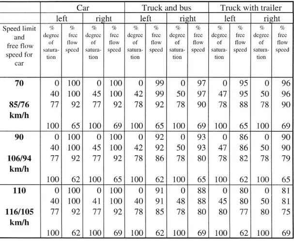
The final results of the above work are set out in Table 7, which shows the speed-flow
relation for all three vehicle types. Table 7 gives the ow per lane in degree of saturation and the speed in percent of the free flow speed for cars. (Note that the speed for heavy vehicles is given in this measure). There are four rows for each speed limit.
Row 1 is the free ow condition (degree of saturation = 0), row 2 is the first
breakpoint, row 3 is the second breakpoint and row 4 gives the capacity limit. The ideal free ow speed for cars for the left and right lane is given for each speed limit, see TableZ in Section 6.4.
Table 7 Speed-flow relation for three vehicle types given in relative numbers.
Car Truck and bus Truck with trailer left ri ht left ri ht left ri ht
Speed limit % % % % % % % % % % % %
and degree free degree free degree free degree free degree free degree free of flow of flow of flow of flow of flow of flow
free flow satura- speed satura- speed satura speed satura- speed satura speed satuia. speed
speed for tion tion tion tion tion tion
car 70 0 100 0 100 0 99 0 97 0 95 0 96 40 100 45 100 42 99 50 97 47 95 50 96 85/76 77 92 77 92 78 92 78 90 78 88 78 90 km/h 100 65 100 69 100 65 100 69 100 65 100 69 90 0 100 0 100 0 92 0 93 0 86 0 90 40 100 45 100 42 92 50 93 47 86 50 90 106/94 77 92 77 92 78 86 78 80 78 82 78 79 km/h 100 62 100 65 100 62 100 65 100 62 100 65 110 0 100 0 100 0 91 0 88 0 80 0 81 40 100 41 100 40 91 48 88 45 80 50 81 116/105 77 92 77 92 78 85 78 80 80 77 80 75 km/h
100
62 100
69 100
62 100 69 100 62 100
69
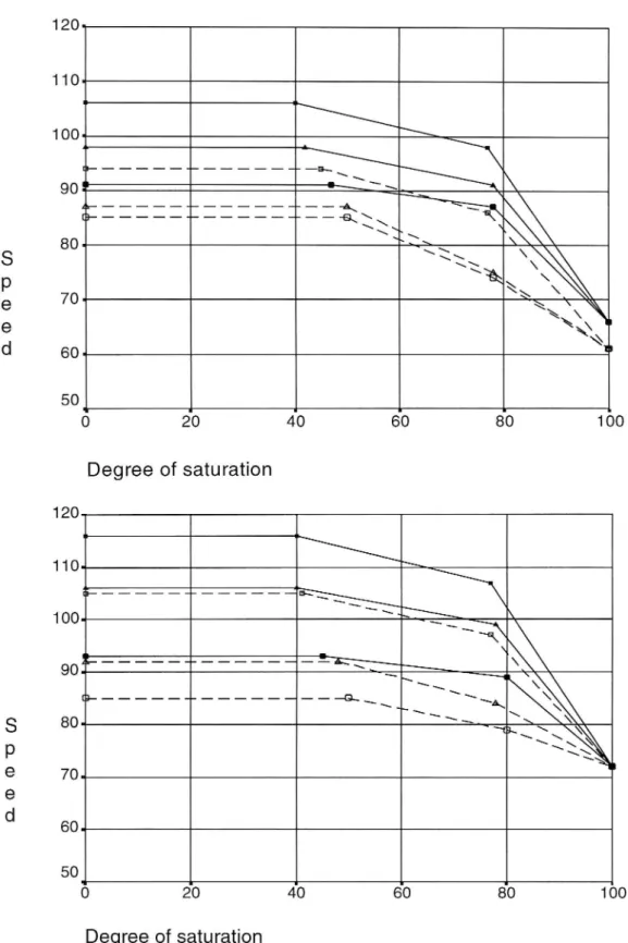
Figure 2 and 3 show plots of the above relations. However, the free flow speed has been allocated to the ideal values shown in the Table 7 above, which give an y-axis in terms of km/h. The x axis is the degree of saturation in percent.
Figures 2 and 3 shows speed ow for both lanes, using a solid line for the left lane and a broken line for the right lane. Plots for all of the three vehicle types are presented.
120 110 100 90
80
=\\\\.\
S H E & XR&::z::3:::::::: E;5\\
\\
p 70
== TQM &
e
*Äx
e
\
\\
d 60
ex
x%
50 . . . . _ O 20 40 60 80 100Degree of saturation
Fig. 2 - Speed-flow relations for three vehicle types at 70 km/h. Three solid lines
for left lane (car, truck and bus, truck with trailer) and three broken lines for the
120 110 100 \ \
90
=\\\\ xxx \
A80 \ :Q:\\ X S» ~\:h;?§l \ \ p 70 ås \
e
xxx
\\\ |e
Q
x; d 60 n 50 0 20 40 60 80 100 Degree of saturation 1200
XXX
100 _X*:Ti:jj>\\E\\\ 90 _____' _____ 3\N\\ & \\\\ X. \\c;
G~\\~_\ \\\,\\ Xx
S 80 .\\ &\\\\\\\\ XP
*lxx
e 70 e d 60 50 0 20 40 60 80 100 Degree of saturationFigure 3 - Speed- ow relations for three vehicle types at 90 km/h (above) and
110 km/h (below). Three solid lines for left lane (car, truck and bus, truck with
9. DISCUSSION AND SUMMARY
One general conclusion is that it is difficult to find clear and significant relations except in a few respects. First, it is evident that with an increasing total ow, an increasing proportion of cars use the left lane. This applies when the total ow exceeds about 3,000 vehicles per hour. Second, this leads to clearly higher speed and capacity values for the left lane. A distribution of cars by lane occurs in such a way that vehicles in the right lane drive at a lower speed and greater time headway compared with cars in the left lane.
In regard to free ow speeds relations with road performance were very ambiguous. Random factors, such as distribution according to purpose of travel and distance to a traffic interchange, in uenced speed to almost as great an extent as road performance. Further, both lane width and hard shoulder width are always reduced on sections
narrower than 11.5 m. Therefore, it is difficult to describe the in uence of individual
factors on road performance on the basis of the material.
The relations at the capacity limit are highly random and difficult to model with the macro expressions that have been applied. This is re ected by the fact that the traffic process is not stationary but instead highly dynamic. This applies in particular to the measuring sites on which the analysis have been concentrated. Most of these sites are characterised by traffic towards city centre and the presence of on-ramps with high
ows downstream or upstream of the measuring site.
Other measuring sites which have not been analysed in the same detail, since no capacity limit was observed, are instead characterised by outbound traffic and the presence of off-ramps with correspondingly high ows downstream or upstream of the measuring site. It appears that this causes considerably less in uence on traffic process on the arterial.
It should be noted that the capacity values reported in Section 7.3 are different for these two types of traffic. Arterials of the first type with predominantly incoming traffic have lower values. The difference is about 200 300 vehicles per hour for both lanes compared with arterials of the second type with predominantly outgoing traffic.
10. REFERENCES
ANUND, P. and SÖRENSEN G. (1995) PREC95, Software for Reduction and Analys
of Traffic Data - Description and Manual (in Swedish) Notat T147. The Swedish Road and Transportation Research Institute (VTI) Linköping, Sweden, 1995.
Highway Capacity Manual (1994) Special Report 209 Third Edition. Transport
Research Board, National Research Council, Washington D.C.