Research Institute of Industrial Economics P.O. Box 55665 SE-102 15 Stockholm, Sweden
info@ifn.se
IFN Working Paper No. 1382, 2021
Artificial Intelligence, Robotics, Work and
Productivity: The Role of Firm Heterogeneity
Fredrik Heyman, Pehr-Johan Norbäck and Lars
Persson
Artificial intelligence, Robotics, Work and Productivity:
The role of Firm Heterogeneity
∗
Fredrik Heyman
Research Institute of Industrial Economics (IFN)
Pehr-Johan Norbäck
Research Institute of Industrial Economics (IFN)
Lars Persson
Research Institute of Industrial Economics (IFN), CEPR and Cesifo
February 11, 2021
Abstract
We propose a model with asymmetric firms where new technologies displace workers. We show that both leading (low-cost) firms and laggard (high-cost) firms increase productivity when automating but that only laggard firms hire more automation-susceptible workers. The reason for this asymmetry is that in laggard firms, the lower incentive to invest in new technologies implies a weaker displacement effect and thus that the output-expansion effect on labor demand dominates. Using novel firm-level automation workforce probabilities, which reveal the extent to which a firms’ workforce can be replaced by new AI and robotic technology and a new shift-share instrument to address endogeneity, we find strong empirical evidence for these predictions in Swedish matched employer-employee data.
Keywords: AI&R Technology; Automation; Job displacement; Firm Heterogeneity; Matched employer-employee data
JEL classification: D2; J24; L2; O33
∗Research Institute of Industrial Economics (IFN), P.O. Box 55665, SE-102 15 Stockholm, Sweden. Email:
fredrik.heyman@ifn.se, pehr-johan.norback@ifn.se, and lars.persson@ifn.se. Fredrik Heyman gratefully acknowledges financial support from the Johan and Jakob Söderbergs Stiftelse and the Torsten Söderbergs Stiftelse. All authors gratefully acknowledge financial support from the Marianne and Marcus Wallenberg Foundation and the Jan Wal-lander och Tom Hedelius Stiftelse. We have benefitted from the feedback provided by participants at seminars and conferences.
1. Introduction
Firms are increasingly able to automate job tasks using advances in robotics, machine learning and other forms of artificial intelligence. Examples include coordinating production and transportation, picking orders in a warehouse and performing automated customer service. We will refer to this technology as Artificial Intelligence and Robotics (AI&R) technology. Recent studies show that AI&R technology affects firms and workers. For instance, Graetz and Michaels (2018) use the variation in robot usage across industries in different countries and find that industrial robots increase productivity and wages but reduce the employment of low-skill workers. Acemoglu and Restrepo (2020) rely on the same IFR data and find robust adverse effects of robots on employment and wages in the US commuting zones most exposed to automation by robots.
However, firms’ incentives to automate will likely differ substantially across different types of firms. Indeed, Syverson (2011), in his overview article, concludes that large and persistent dif-ferences in productivity levels across businesses are ubiquitous and to a large extent depend on firm-specific assets. Berlingieri et al. (2017) provide evidence on the increasing dispersion in wages and productivity using microaggregated firm-level data from 16 countries. These results notwith-standing, we have little systematic knowledge about how different types of firms may implement these new AI&R technologies and how this may affect productivity and hirings and firings in dif-ferent types of firms. The purpose of this paper is to provide more knowledge on these matters.
To capture these elements in an AI&R-driven industrial restructuring processes, we propose a model in which firms differ in their inherent productivity due to different firm-specific assets such as patents, know-how or human capital. We refer to firms with inherently high productivity as leading firms and firms with inherently low productivity as laggard firms. Firms competing in imperfectly competitive product markets may then use advances in AI&R technology to automate their production and displace labor in the production process. We refer to this labor type as production employees.
We show that only laggard firms increase the hiring of production employees when investing in the new AI&R technology. The reason is that increasing investment in the new AI&R technology has two effects on the demand for production employees. First, the implementation of the new AI&R technology reduces per unit of output demand for production employees–this is the displacement effect. However, there is also a second effect–the output effect–that increases the demand for production employees. For laggard firms, the output effect dominates the displacement effect, since their inherently lower output reduces their incentives to invest significantly in the new AI&R technology.
We then turn to our empirical analysis. Sweden has been at the forefront of the implementation of new AI&R technology in its business sector. Sweden is, therefore, a suitable country to study the influence of new AI&R technology on labor demand and productivity on a larger scale. Our analysis uses comprehensive and detailed Swedish matched employer-employee data from 1996 to 2013. The use of detailed information on firms, plants, and individuals working for the firms makes it possible to analyze issues related the impact of the implementation of new AI&R technology on
job and productivity dynamics in greater detail than is possible in most other international studies. The starting point in our empirical analysis is that the implementation of AI&R technology will affect firms’ behavior in terms of their investments in the new technology, the composition of workers in different occupations, and performance in terms of productivity. However, lacking information on investments in AI&R technology, we first calculate a novel measure of a firm’s workforce automation probabilities, which is based on estimated automation probabilities at the occupational level derived by Frey and Osborne (2017). This firm-specific measure reveals the extent to which a firm’s workforce can be replaced by new AI&R technology. We then use this measure to identify how the implementation of AI&R affects the occupational mix and productivity development in different types of firms.
To this end, we first note that our model predicts that only laggard firms increase their hiring of production workers, but all firms increase productivity when implementing AI&R technology. This prediction implies that only in laggard firms will an increase in the firms’ exposure to automation be positively correlated with increased productivity–in leading firms, an increase in firm exposure to automation will be negatively correlated with increased productivity.
To test these predictions, we estimate panel data models with firm fixed effects, regressing productivity on firms’ exposure to automation, their share of skilled workers and the interaction between the exposure to automation and the skill share (plus additional controls). From the theory, we can show that a high skill share of the workforce (i.e. a high share of employees with a university degree) is associated with leading firms, while a low skill share is associated with laggard firms. As predicted from the theory, our basic OLS estimates show that an increase in the automation probability–or exposure to automation–is associated with an increase in productivity in laggard firms, i.e. firms for which the skill share is sufficiently small. As also predicted, in leading firms, i.e. firms in which the skill share is high, an increase in the exposure to automation is associated with a reduction in productivity.
As our theory suggests, it is likely that we have an omitted variable problem associated with the relation between productivity and workforce automation probabilities: The AI&R technology will not only affect productivity through its effect via hiring and firing but also directly through an efficiency effect. To address this potential endogeneity problem, we use aggregate changes in the employment structure and workforce automation probabilities as a shift-share instrument for firm-level workforce automation probabilities. When using this instrument, we find that IV results are remarkably similar to the OLS results in that productivity and exposure to automation are positively (negatively) correlated when the skill share is sufficiently low (high).
Our paper relates to the literature that examines the impact of investment in AI&R technology on employment. Worker displacement plays a central role in this literature, as machines take over tasks previously performed by humans. (Autor et al.2003; Acemoglu and Autor 2011; Acemoglu and Restrepo 2018a,b, 2019a,b; Benzell et al. 2016; Susskind 2017). The empirical work on the implications of AI&R technology investments on labor demand has thus far mostly focused on robotics. Using similar IFR data as in Graetz and Michaels (2018) and Acemoglu and Restrepo
(2020), Dauth et al. (2017) analyze Germany. They find no evidence that robots cause total job losses but that they do affect the composition of aggregate employment. While industrial robots have a negative impact on employment in the manufacturing sector, there is a positive and significant spillover effect as employment in the non-manufacturing sectors increases. They also report that robots raise labor productivity. Some recent papers take the analysis to the firm level. Koch et al. (2019) show that firms that adopt robots experience net employment growth relative to firms that do not, and Dixon et al. (2019) find that a firm’s employment growth increases in its robot stock. Humlum (2019) uses Danish firm-level robot data and finds that increased robot usage leads to an expansion of output, layoffs of production workers, and increased hiring of advanced employees. Finally, Aghion et al. (2020) use microdata on the French manufacturing sector. Based on event studies and a shift-share IV design, their estimated impact of automation on employment is positive, even for unskilled industrial workers. Moreover, the industry-level employment response to automation is positive and significant only in industries that face international competition.
We contribute to this literature by proposing a model of automation with heterogeneous firms. We show that both leading and laggard firms increase productivity when automating, but only laggard firms increase the hiring of automation-susceptible employees.1 The reason is that laggard firms have low investment incentives, which results in a small displacement effect, and the output-expansion effect will therefore dominate. Seamans and Raj (2020) summarize the recent literature on AI, labor and productivity and highlight the lack of firm-level data on the greater use of AI. We contribute to this literature by proposing a new measure of workforce exposure to AI&R in a firm based on the work by Frey and Osborne (2017). This enables us to examine the effects on firms of different types and the role of market structure in AI&R investments on a more general level. We find support for these mechanisms in detailed matched employer-employee data for Sweden spanning the period 1996-2013, using a shift-share IV design to address endogeneity problems. In particular, we find that leading and laggard firms will have different productivity developments and in particular behave differently in their hiring of employees in occupations susceptible to automa-tion.
This paper also contributes to the literature on technological development and productivity development, which has demonstrated that measured productivity growth over the past decade has slowed significantly (Syverson, 2017). Productivity differences between frontier firms and average firms in the same industry have been increasing in recent years (Andrews et al., 2016; Furman and Orszag, 2015). Moreover, a smaller number of superstar firms are gaining market share (Autor et al., 2017), while workers’ earnings are increasingly tied to firm-level productivity differences (Song et al., 2015). We contribute to this literature by examining the effects of AI&R investments on firms of different types. We show that both leading firms (low-cost firms) and laggard firms (high-cost firms) increase productivity when implementing AI&R technology but that only laggard firms hire more automation-susceptible workers.
1
Besen (2019) proposes a demand satiation model that can explain the growth and subsequent decline in employ-ment over time when a new technology is introduced.
The paper proceeds as follows. Section 2 presents the theoretical model that we use to examine how investment in AI&R technology affects leading and laggard firms’ productivity and employment development and to derive predictions for our empirical analyses. In Section 3, we conduct the empirical analysis. Section 4 discusses the policy implications. Finally, Section 5 concludes the paper. In the Appendix, we present several extensions to the model, e.g., relaxing some of the assumptions made in the benchmark model.
2. The model
2.1. Preliminaries
Consider an industry with firms indexed = {1 2 }, each producing a single differentiated product. A representative consumer has quadratic quasilinear preferences over consumption of the products and the consumption of an outside good
(q) = X =1 − 1 2 ⎡ ⎣ X =1 2+ 2 X =1 X 6=1 ⎤ ⎦ + 0 (2.1)
where 0 is a firm-specific demand parameter, is the consumption of product 0 is the
consumption of the outside good, and ∈ [0 1] captures the degree of product differentiation. The representative consumer faces the budget set
X
=1
+ 0 = (2.2)
where is exogenous consumer income and is the price of product . The price of the outside
good is normalized to unity. Solving for the amount of consumption of the outside good, 0, from
the budget constraint (2.2), the direct utility in (2.1) can be rewritten as (q) = X =1 (− ) − 1 2 ⎡ ⎣ X =1 2+ 2 X =1 X 6= ⎤ ⎦ − (2.3)
Taking the first-order condition for utility maximization,
= 0, we obtain the inverse demand
facing each firm
= − −
X
6=
= {1 2 } (2.4)
maximization problem of firm is max {} = () · | {z } Revenues − · ( ) | {z }
Wage costs from production
− () | {z } Installation costs − |{z} Fixed cost (2.5) : () = − (2.6) : ( ) = () · (2.7) : () = − 0 (2.8) : () = 2 2 0 (2.9)
The first row depicts the direct profit that the firm is maximizing by optimally choosing output, ,
and the amount of AI&R technology, ,: The first term is the firm’s revenues, () ·; the second
term depicts costs for labor used in production, · ( ) where is the exogenous wage for
production workers (given from the labor market), and (·) is the number of unskilled production
workers; the third term depicts installation costs for the AI&R technology, (); and the last term
depicts the wage costs for a fixed number of (high skilled) workers needed to use AI&R technology, .
An important component of the labor cost to produce units of output is the per unit
require-ment of labor, (), since the total number of production workers is ( ) = () from (2.7).
As shown in (2.8), if the firm invests more in AI&R technology , this will reduce the number
of production workers needed to produce one more unit at rate . Finally, from (2.9), there are quadratic installation costs for the AI&R technology, () = 22.
The exogenous industry variables and characterize the efficiency and the cost of AI&R technology. It is then useful to define the following exogenous variable, which we will denote the return to investing in the AI&R technology2
=
2
(2.10)
Intuitively, the return to investing in AI&R technology is higher when this technology is more efficient in replacing labor (i.e., when is higher), and when it becomes less expensive to invest in AI&R technology (i.e., when is lower). The variable will be a useful tool to study how investments in AI&R technology affect productivity and the composition of employment within firms.
To proceed, we normalize the wage for production workers to unity, = 1. In the Appendix, we show that this normalization does not qualitatively affect our results. As we will discuss below, in the Appendix, we also provide an extension of the model where the demand for skilled workers increases with investments in the AI&R technology. Additionally, the Appendix also contains an extension where we allow for the impact of competition in the product market.
We now return to the profit maximization problem for firms in (2.5). Consider the following
setting: In stage 1, a firm invests in the new AI&R technology, . In stage 2, given its investments
in technology, , the firm sells units of its product to consumers. To solve (2.5), we use backward
induction.
2.2. Stage 2: Product market
Using the inverse demand (2.6), the unit labor requirement (2.6) and the investment cost for the AI&R technology (2.9) in (2.5), we obtain
max {} = (− ) | {z } Revenues − (− ) | {z } Wage costs − 22 |{z} Installation cost − |{z} Fixed costs (2.11)
The optimal output is given from the first-order condition
= − − (− ) = 0 = {1 2 } (2.12)
with associated second-order condition 2
2
= −2 0
From (2.12), we can solve for the optimal output ∗() =
− (− )
2 (2.13)
To ensure that the firm produces output–even without investments in the new technology–we will assume that . Note that the firm will produce more output ∗ when having invested
more in the AI&R technology, To explore this mechanism in greater detail, it is instructive
to rewrite the first-order condition into the familiar form equating marginal revenue ( ) and
marginal cost ( ), with marginal revenue expressed as a function of a firm’s price elasticity of
demand, = ∙ 1 −1 ¸ | {z } = |{z} (2.14)
A firm with market power will choose output such that the price elasticity of demand is larger than unity, i.e., 1. This fact implies that if increased investments in AI&R technology induce
a firm to reduce its product market price, the increase in demand will cause the output to rise. In the analysis below, we will examine (i) whether the output expansion effect can compensate for the replacement effect, i.e., if labor demand can increase when investments in AI&R technology increase, and (ii) if so, in which firm type this mechanism is at play.3
3Bessen (2019) shows that labor demand in the textile industry in the 19th century grew for an extended period
despite considerable improvements in productivity from labor-saving technologies. He also develops a model that explains this pattern by a highly elastic demand for textiles.
2.3. Stage 1:Investing in the AI&R technology
How much will a firm then invest in the AI&R technology, ? Substituting the optimal quantity,
∗(), from (2.12) into (2.11), we obtain
max {} () = [− ∗()] ∗() | {z } Revenues − (− ) ∗() | {z } Wage cost − 22 |{z} Installation cost − |{z} Fixed cost (2.15)
Using the envelope theorem, the first-order condition is ()
= ∗(∗) − ∗ = 0 (2.16) From (2.16), we can link the optimal level of investments in the AI&R technology, ∗, to optimal output ∗(∗)
∗ = ·
∗
(∗) (2.17)
Combining (2.10), (2.13) and (2.17), we can solve for the equilibrium level of AI&R technology, ∗()
∗() = ·
−
2 − 0 (2.18)
where it is easily checked that 2 − 0 is required from the second-order condition associated with (2.15).
Combining (2.6)-(2.8), (2.17) and (2.18), we can finally solve for a firm’s equilibrium quantity, ∗
(), equilibrium price, ∗(), equilibrium unit requirement, ∗(), and the equilibrium labor
demand, ∗(), all as functions of the return to investing in AI&R technology, .
∗() = − 2 − 0 (2.19) ∗() = − ∗() = +2−− 0 (2.20) ∗() = − · ∗() = · 2− 2− 0 (2.21) ∗() = ∗() · ∗() = · (−) 2− (2−)2 0 (2.22)
where we assume that the return to investing in AI&R technology is not excessively high to ensure that the unit labor requirements for all firms are always strictly positive, i.e., ∈ [0 max ) for
∀, where max = 2
. Furthermore, the return to investing in the new technology is capped by
restricting the product market price for all firms to be strictly positive, i.e., + − 0 for
2.4. Comparative statics: Increasing return to investing in AI&R technology
Suppose that technological developments increase automation possibilities by increasing the re-turn to investing in AI&R technology, defined in (2.10). How will this affect firms in terms of investments in AI&R technology, labor productivity and the employment of production workers? 2.4.1. Impact on investments in AI&R technology
From (2.18), we have the following straightforward result:
Lemma 1. The amount of AI&R technology investment by firm ∗() is strictly increasing in the return to investing in new AI&R technology (either because the new technology becomes less expensive, ( ↓), or because new technology becomes more efficient ( ↑)
Intuitively, increased return to investing in AI&R technology increases the level of AI&R tech-nology used in equilibrium.
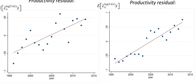
2.4.2. Impact on labor productivity and value added per employee
Labor productivity Increased investments spurred by a higher return to investment in the AI&R technology should increase productivity in the firm. We define labor productivity as output per worker, which we will label ∗(). Using (2.7), we have
∗() = Output z }| { ∗() ∗ () | {z } Production + |{z} Non-production | {z } Total employment = 1 ∗ () + ∗ () | {z }
Total unit labor requirement
(2.23)
Taking logs in (2.23) and differentiating with respect to , we can derive the following elasticity expressions, which show how an increase in the return to investing in AI&R technology affects labor productivity ∗() ∗() = ∗ ()·
Output expansion effect :(+)
z }| { µ ∗() ∗ () ¶ − Replacement effect:(−) z }| { µ ∗ () ∗ () ¶ 1 + ∗ () 0 (2.24) The expression in (2.24) shows that labor productivity is strictly increasing in the return to investing in AI&R technology from two distinct effects: an output-expansion effect (weighted by relative employment) and a replacement effect.
The output-expansion effect is strictly positive, since from (2.19), we have ∗ () · ∗() = 2 − 0 (2.25)
The replacement effect is strictly negative, since from (2.21), we have ∗() ∗() = − 2 − (2 − ) ³ 2 − ´ 0 (2.26)
Intuitively, when the return to investment, , increases, firms respond by investing more in the AI&R technology, i.e., ∗()
0 from Lemma 1. This reduces the unit labor requirements ∗()
from (2.8), reducing marginal costs, which, in turn, increases output ∗
() from (2.13). With larger
output and fewer workers needed to produce each unit of output, labor productivity is raised. We summarize these results as follows:
Proposition 1. An increase in the return to investing in the AI&R technology strictly increases labor productivity, ∗
∗
0
Value added per worker In the empirical analysis presented in the next section, we will not have data on unit labor requirements and output levels (typically not observed in firm-level data). We will have data on firms’ revenues and costs. We will therefore use value added per employee as our productivity measure. How is this alternative measure affected when the return to investing in AI&R technology becomes more profitable?
Let ∗() denote the reduced-form value added per employee, and let ∗() = ∗() · ∗() denote revenues. Without materials in our model, value added per worker can then be written as the average revenue per total labor hour used:
∗() = Revenues z }| { ∗() ∗() + | {z } Total employment = Average revenue z }| { ∗() ∗ () + ∗ () | {z }
Total unit labor requirement
(2.27)
where we use (2.7) in the last term.
Taking logs in (2.27) and again differentiating with respect to , we obtain ∗() ∗ () = ∗ () ∗ () | {z }
Labor productivity effect: (+)
+ ∗ () ∗ () | {z } Price effect: (-) (2.28)
Thus, the percentage change in value added per employee from a one-percent increase in the return to investing in AI&R technology is simply the percentage change in the unit labor requirement net of the percentage change in the product market price. We already know from (2.24) that the labor productivity effect is strictly positive from the combined influence of the labor-replacement and output-expansion effects. However, from the output-expansion effect being strictly positive in (2.25), there must be a reduction in the product market price from (2.6). From (2.20), we can show
that the price effect is negative ∗() ∗ () = − − (2 − ) (+ − ) 0 (2.29)
In sum, a higher return to investing in AI&R technology increases a firm’s labor productivity– however, the higher return also reduces the price of the firm’s good or service. We show in the Appendix that the labor productivity effect still dominates, and value added per employee will increase in the return to investment in AI&R technology, i.e., ∗()
∗
() 0 in (2.28).
Value added per employee will, of course, underestimate the true increase in labor productivity from new technologies. In our setting, this is not a serious problem since our focus is on inferring whether productivity improvements from AI&R investments can occur with rising employment in occupations susceptible to automation and–if so–in which type of firms this arises. To summarize: Corollary 1. An increase in the return to investing in the AI&R technology also strictly increases value added per employee, ∗
∗
0
2.4.3. Impact on employment
How is employment affected when investments in AI&R technology become more profitable? Since the employment of non-production workers is by assumption fixed (this assumption is relaxed in the next section), we can focus on the impact of production workers that are susceptible to being replaced by technology. Taking logs of the reduced-form employment, ∗() = ∗() · ∗(), and then differentiating with respect to the return , we obtain
∗() · ∗ = ⎛ ⎜ ⎜ ⎜ ⎝ ∗() · ∗() | {z } Displacement effect (-) + ∗ () · ∗() | {z } Output effect (+) ⎞ ⎟ ⎟ ⎟ ⎠ (2.30)
More profitable investment opportunities in labor-saving AI&R technology implies that fewer work-ers are needed per unit of output produced–however, more workwork-ers are also needed because output increases: From the displacement effect in (2.26), we know that a higher return, , leads to a lower unit labor requirement, ∗()
∗
() 0. However, improving technological opportunities also
in-creases output, that is, from the output-expansion effect in (2.25), ∗()
∗
() 0.
Which of these two opposing forces–the displacement effect or the output-expansion effect– dominates? Inserting (2.30) and (2.25) into (2.30) and simplifying, we obtain
∗ () · ∗ = 2 · ³ 2 − ¡ 1 +2¢´ (2 − )³2 − ´ R 0 (2.31)
Definition 1. Firm i is a "laggard firm" if it has a relatively high innate cost, i.e.,
∈ (1 2) In
contrast, Firm i is a "leading firm" if it has a relatively low innate cost, i.e.,
2.
We can then state the following proposition: Proposition 2. Define the cutoff = (4
) ³ 1 −12 ´
. Then, the following holds: 1. (Laggard firm) If
∈ (1 2) holds, an increase in the return to investing in AI&R technology
0 leads to the following:
a.) An increase in employment, ∗()
∗ () 0, if ∈ [0 ) b.) No change in employment, ∗() ∗ () = 0, if =
b.) A decline in production employment, ∗()
∗ () 0 if ∈ ( max ) 2. (Leading firm) If
2 an increase in the return to investing in AI&R technology, 0
always reduces employment, ∗()
∗
() 0.
Let us explain the intuition in Proposition 2. Since the output-expansion effect, i.e., the elas-ticity ∗()
· ∗
() is independent of firm characteristics (c.f. Equation 2.25), the heterogenous
employment of the different firm types in Proposition 2 can be understood from the displacement effect, ∗
∗
(). It is then useful to rewrite the displacement effect as follows:
∗ ∗ () = − ∗ () ∗ () · µ 2 2 − ¶ 0 (2.32)
where we have used (2.21) and (2.25).
Faced with weak consumer demand (i.e., low ) and weak cost efficiency (i.e., high ) laggard
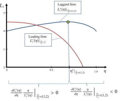
firms will choose a lower output, ∗() (c.f. Equation 2.19). This implies a weak incentive to invest in the new AI&R technology since any reduction in the unit labor requirement will affect few units of output (c.f. Equation 2.17). The low investments in the labor-saving technology then translate into a high unit labor requirement, ∗() (c.f. Equation 2.8). As shown in (2.32), at a low output level and high unit labor requirements (i.e., at a low ratio ∗()∗()), the displacement effect is weakened. The output-expansion effect therefore dominates in (2.30), and substitutable production employment increases despite increased investments in labor-saving AI&R technology. The employment locus for a laggard firm, ∗()|
∈(12), is shown in Figure 2.1, where a higher
return to investing in AI&R technology increases production employment as long as the initial return is not too high.
In contrast, under greater consumer demand (i.e., a higher ) and higher cost efficiency (i.e., a
lower ) leading firms produce more output, providing a stronger incentive to invest in labor-saving
technology which, ultimately, yields a low unit labor requirement. From (2.32), at a high level of production and a low unit labor requirement (i.e., at a high ratio ∗()∗()), the displacement
5 4 3 2 0 0.5 1.0 Li∗|ai ci∈1,2 Li∗|ai ci2 Laggard firm: Leading firm: Li iL|ai ci∈1,2 dLi∗ d Li∗ ai ci∈1,2 0 dLi∗ d Li∗ aici∈1,2 0 ( A higher return to invest in the AI&R
technology increases production employement in a laggard firm)
( A higher return to invest in the AI&R technology decreases production employement in a laggard firm)
Figure 2.1: Illustrating Proposition 2. Parameter values are = 6 and = 3 for a leading firm and = 4 for a laggard firm.
effect is now strengthened: The output expansion effect is now dominated by the displacement effect in (2.30), and substitutable production employment declines when investments in labor-saving AI&R technology increase. The employment response for a leading firm is illustrated by the employment locus ∗()|
2 in Figure 2.1. In contrast to a laggard firm, a higher return to
investment in AI&R technology always reduces employment in the leading firm. 2.5. Empirical predictions
Let us now derive empirical predictions from the model to be tested in the next section. 2.5.1. Labor productivity and employment susceptible to automation
Combining Propositions 1 and 2, our first prediction concerns how productivity (as measured by value added per employee) and production employment are related when firms increase their investments in the AI&R technology.
Prediction 1: Suppose that the return to investing in AI&R technology, increases. Firms will then respond by increasing their investments in AI&R technology, ∗()Then:
(i) For a "laggard firm",
∈ (1 2) given that the return to investment is not too high, ∈ [0
),
increased investment in the new AI&R technology lead to a positive correlation between pro-duction employment, (), and value added per employee, (), as increased investment
(ii) For a "leading firm", 2, increased investment in the new AI&R technology leads to a
negative correlation between production employment, () and labor productivity, ().
Part (ii) states that in more efficient leading firms, there is a negative correlation between production worker employment and productivity. In these firms, the displacement effect of the new technology dominates the output-expansion effect in (2.30), and labor demand falls when productivity increases. In contrast, Part (i) states that in less efficient laggard firms, the correlation between labor productivity and the employment of production workers (who are substitutable for AI&R investments) is positive. That is, increasing firm-level productivity is associated with higher employment of production workers–in the latter type of firm, the output-expansion effect of increased AI&R investments dominates the displacement effect in Equation (2.30).
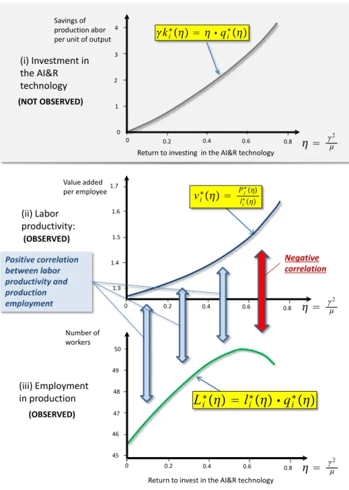
These predictions are illustrated in Figure 2.2 and Figure 2.3, where the top panels show a firm’s investments in AI&R technology, ∗() the middle panels depict its labor productivity, ∗() and the bottom panels depict its production employment, ∗(). As shown by the horizontal axis, all three endogenous variables are functions of the return to investment in the AI&R technology, . The top panels in Figure 2.2 and Figure 2.3 are shaded to illustrate that we–in the empirical analysis in the next section–do not observe the actual AI&R investments.
Thus, we will test the predictions from the model from the relationship between labor pro-ductivity and employment. We then assume a process whereby automation possibilities increase over time, i.e., the return to investing in new AI&R technologies , rises over time. In leading firms, increasing (unobserved) investments in the new AI&R technology lead to higher productivity associated with falling production employment. From the two lower panels in Figure 2.2, this pro-duces a negative correlation between labor productivity and production employment. In contrast, from the lower panels in Figure 2.3, increasing (unobserved) AI&R investment produces a positive correlation between labor productivity and production employment in laggard firms.
2.5.2. Firm heterogeneity
Prediction 2.5.1 tells us that the correlation between productivity and the employment of production workers should differ between firm types: In laggard firms, productivity and the employment of production workers susceptible to automation are positively correlated; when laggards respond to better automation possibilities by investing more in new technology, increased productivity is accompanied by increased employment in production. However, in leading firms, the increase in productivity–spurred by increased investments in new technology–entails reduced production employment.
How can we then identify firm types in data without detailed firm-level information on costs and demand (i.e., the parameters and )? Our main proxy for firm type in the empirical analysis will
be the share of skilled workers in a firm, under the assumption that leading firms should be firms with higher skill intensity and laggard firms should be firms with lower skill intensity. Suppose that production workers are essentially less skilled workers. From the assumption of a fixed number of
2
2
2 Return to invest in the AI&R technology
Return to invest in the AI&R technology
0.2 0.4 0.6 0 0 0.8 1 2 3 4 5 6 2 3 0.2 0.4 0.6 0 0.8 0.2 0.4 0.6 0 0.8 50 40 vi∗ Pi∗ li∗ ki∗ qi∗
L
i∗ l
i∗ q
i∗
Value added per employee Savings of production labor per unit of output Number of workers 35 (i) Investment in the AI&R technology (ii) Labor productivity: (iii) Employment in production (NOT OBSERVED) (OBSERVED) (OBSERVED) Negative correlation between labor productivity and production employmentFigure 2.2: Illustrating a negative correlation between production worker employment and produc-tivity.
(i) Investment in the AI&R technology (ii) Labor productivity: (iii) Employment in production 2 2 (NOT OBSERVED) Positive correlation between labor productivity and production employment Negative correlation
Return to investing in the AI&R technology
0.2 0.4 0.6 0.8 0 0 1 2 3 4 0.2 0.4 0.6 0.8 0 1.3 1.4 1.5 1.6 1.7 2 0.2 0.4 0.6 0.8 0 45 46 47 49 50 48
Return to invest in the AI&R technology
vi∗ Pi∗ li∗ ki∗ qi∗ Value added per employee Savings of production abor per unit of output Number of workers (OBSERVED) (OBSERVED)
L
i∗ l
i ∗ q
i ∗
Figure 2.3: Illustrating a positive correlation between production worker employment and produc-tivity.
high-skilled non-production workers, , the share of high-skilled workers in firm employment in the
model is simply
∗() = ∗() +
(2.33)
From Proposition 2 and (2.33), it follows that when the return to investment in new technologies becomes sufficiently high, leading firms will have a higher skill intensity than laggard firms: ∗() is declining in leading firms, while ∗
() is increasing in laggard firms (unless becomes too high).
By taking logs in (2.33) and differentiating with respect to , we can examine how skill shares change when the return to investment in the new technology increases
∗() ∗() = − ∗() ∗()· (1 − ∗ ()) (2.34)
Thus, when the return to investing in AI&R technology increases, the percentage change in the share of skilled workers, ∗()
∗
() and the percentage change in production worker employment,
∗ ()
∗
(), move in opposite directions.
The inverse relationship in (2.34) leads to our second prediction:
Prediction 2: Suppose that Prediction 1 holds and ∗() 0. Then, from (2.34), it follows that: (i) In a "laggard firm",
∈ (1 2), if the return to investment is not too high, ∈ [0
), increased
investments in the new AI&R technology lead to a negative correlation between skill intensity ∗() and value added per employee, () .
(ii) In a "leading firm",
2, the increased investments in the new AI&R technology lead to a
positive correlation between skill intensity ∗() and value added per employee, ().
On a final note, Predictions 1 and 2 build on a very simple structure of a firms’ workforce composition, in particular assuming a fixed labor requirement of skilled non-production workers and variable employment of less skilled production workers. A more elaborate assumption would be to assume that the cost of skilled non-production workers is · (+ ), so that an additional
0 of skilled workers are needed for each unit of investment in AI&R technology, in addition
to the fixed requirement, . In Appendix A.2, we show how Predictions 2.5.1 and 2.5.2 also hold
when increased investment in AI&R technology also increases non-production high-skilled workers, under mild restrictions on
3. Empirical analysis
Our aim in the empirical section is to estimate how AI&R technology investments affect productivity and the relationship between productivity and the employment of workers susceptible to being replaced by AI&R technology. The challenge is to examine these relationships without detailed information on firms’ investments in AI&R technology and firms’ demand and cost conditions.
This section first describes the data and how we measure worker susceptibility to automation and firm heterogeneity. In the next section, we present the estimation equation and explain how we capture the model’s prediction of how firm heterogeneity affects the correlation between pro-ductivity and the employment of workers susceptible to being replaced by the AI&R technology. We then present our empirical results.
3.1. Data
We base our analysis on detailed, register-based, matched employer-employee data from Statistics Sweden (SCB). The database comprises firm, plant and individual data, which are linked with unique identification numbers and cover the period from 1996 to 2013. Specifically, the database consists of the following parts:
(i) Individual data The worker data contain Sweden’s official payroll statistics based on SCB’s annual salary survey and are supplemented by a variety of registry data. They cover detailed in-formation on a representative sample of the labor force, including full-time equivalent wages, work experience, education, gender, occupation, employment, and demographic data, among other char-acteristics. Occupations are based on the Swedish Standard Classification of Occupations (SSYK96) which in turn is based on the International Standard Classification of Occupations (ISCO-88). Oc-cupations in ISCO-88 and SSYK96 are grouped based on the similarity of skills required to fulfill the duties of the jobs (Hoffmann, 2004).
(ii) Firm Data The firm data contain a large amount of firm-level data, including detailed accounts, productivity, investments, capital stocks, profits, firm age, and industry affiliation, among other characteristics. The dataset includes all firms with production in Sweden, and in our analysis, we use firms with at least ten employees.
(iii) Plant data The plant data contain detailed plant-level information such as employee demo-graphics, salaries, education, and codes for company mergers, closures, formations, and operational changes. The dataset covers all plants in Sweden. Plant-level data are aggregated at the firm level. 3.1.1. Firm heterogeneity
Section 2.5.2 showed how we can use the share of skilled workers as a proxy for firm type: Firms with a higher share of skilled workers are to a higher degree "leading firms"; firms with a lower share of skilled workers are to a higher degree "laggard firms" (we explain the exact cutoff in the next section). From the matched-employer employee data, we thus calculate the share of employees in a firm with tertiary education, labelled _. As a robustness check, we will also explore
a number of other variables to measure firm heterogeneity, such as the mean years of schooling of a firm’s employees, the mean age of the employees, and the firm’s age.
3.1.2. Workers’ susceptibility to substitution
In the empirical analysis, we need a firm-level measure that captures how new technologies affect firms’ decisions to hire workers susceptible to automation. To highlight the results, we made some simple assumptions regarding labor inputs in our theoretical model–essentially, less skilled blue-collar workers can be replaced by labor-saving automation (the use of the AI&R technology), whereas white-collar workers either cannot be replaced (as they are used in fixed numbers), or they are in higher demand when automation increases. In the empirical analysis, we need a firm-level measure that captures how firms hire workers in many occupations that differ in susceptibility to automation.
Frey and Osborne (2017) compute the probability that a job will be replaced by computers or robots. They predict the computerization probabilities for 702 US occupations, where the predicted risk can be interpreted as the risk that an occupation will be automated within 10 to 20 years. The authors use an objective and a subjective assessment of the occupation-specific automation probability. The objective assessment is based on combinations of required knowledge, skills and abilities for each occupation and ranks the occupations’ likelihood of automation based on this. The subjective ranking categorizes (a subset of the) occupations on the basis of the different tasks they entail. The assessments are based on occupational characteristics and qualifications in the O*NET database, developed by the US Department of Labor. The O*NET database covers almost 1,000 occupations, and for each occupation, there are 300 variables. The variables describe the daily work, skills and interests of the typical employee. These descriptive variables are organized into six different main areas: Characteristics of the Performer, Performer Requirements, Experience Requirements, Occupation-specific Information, Labor Characteristics and Occupational Require-ments. To obtain a probability measure for each occupation, Frey and Osborne use a Gaussian process classifier to identify factors that increase or reduce the ability to computerize a profession. Based on this analysis, the authors provide an occupation-specific automation probability (see Frey and Osborne (2017) for further details).
Frey and Osborne calculate these automation probabilities for the US SOC2010 occupational classification. This classification is not used in Sweden, nor in the EU, and there is no direct translation from the SOC2010 classifications to the Swedish counterpart SSYK96 (ISCO-88). To make use of the automation probabilities provided by Frey and Osborne, we first translate the US classifications to the European occupational code, ISCO08, which in turn can be translated to the Swedish SSYK96 code.4 Given that our data on occupations at the SSYK96 level are available for the years 1996-2013, our emprical analysis will be based on this time period. The occupations most susceptible to automation include machine operators and assemblers and various office clerks, while
4
There are a few issues with this translation. The US code is more detailed than both the EU and Swedish occupational classifications, i.e., some European codes include several US occupations (and vice versa in some cases). We account for this by using occupational employment weights from the United States (Bureau of Labor Statistics, BLS) and from SCB, when there is no 1:1 relationship between US and European occupations. Furthermore, we use the new Swedish occupational classification SSYK2012 for translating ISCO08 to SSYK96. While SSYK2012 is almost identical to ISCO08, differences exist; in these cases, we use different methods to convert the occupational codes.
low automation risk jobs include managers of small enterprises, science professionals and legislators and senior officials.
To obtain a firm-level measure of how susceptible workers in our Swedish firm are to automa-tization, we assume that firms can employ workers from = {1 2 3 } SSYK96 occupations at the 3-digit level ( = 109), where each occupation is associated with an automation probability, which is the converted automation probability from Frey and Osborne (2017). We then
calculate the workforce exposure to automation in firm at time , as
=
X
=1
· (3.1)
where is the share of employees in firm i in occupation j at time t, which is used as a weight
for the automation probability for workers in a particular occupation, . The average risk–or
the average exposure–to automation is thus formed by multiplying the share of employees in an occupation, ∈ [0 1], by the automation probability of that occupation, ,and then summing
over all occupations that are represented within firm . Since the probability of automation for an occupation, , is a time-invariant measure, all variation over time in the exposure to
automation–or average risk of automation–in a firm, , will originate from changes in the
composition of occupations, .
Note that an increase in must be due to a change in the composition of employees within
the firm towards occupations that have a higher probability of automation–in the simple theory, this would capture "laggard firms" increasing their employment of production workers. Conversely, a decrease in must be due to a change in the composition of employees within the firm such
that a smaller share of employees are found in occupations that have a lower probability of being automated –in theory, this would correspond to "leading firms" decreasing their employment of production workers in the theoretical model.
From the theory, we should also expect a negative correlation between and _.
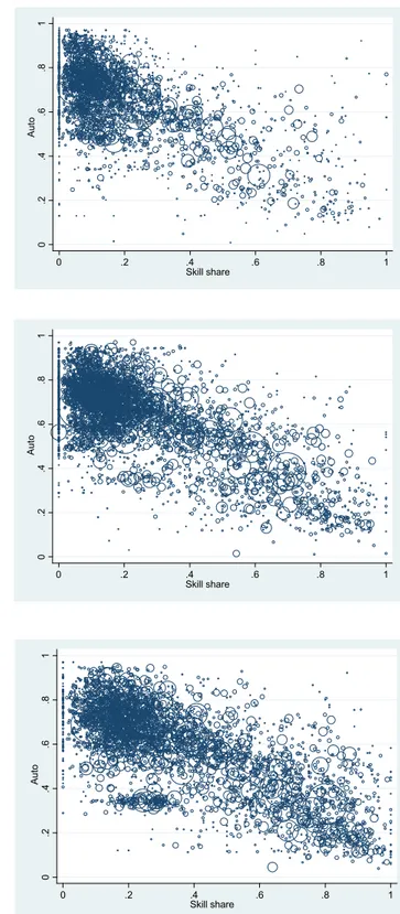
A potential concern regarding the execution of the empirical analysis is a perfect negative correlation between these variables. However, this seems unfounded given multiple types of occupations (where there are also many occupations that require higher education that have relatively high risk of automation). To illustrate this, in Figure 3.1, we plot–for the years 1996, 2004 and 2013–each firm’s combinations of the share of skilled workers, _, on the x-axis and workforce
exposure to automation, , on the y-axis for Swedish firms with at least ten employees. Firm
size in terms of the log number of employees is indicated by the size of the circle surrounding each observation.
Several observations emerge from the three panels in Figure 3.1. First, while workforce exposure to automation and the share of skilled workers are negatively correlated, there is far from a perfect negative correlation. Second, in particular, at the beginning of our period of study, many firms cluster in the area up to the top left with a workforce with high exposure to automation and a lower share of skilled workers. These firms are candidates for the "laggard firm" category in our
0 .2 .4 .6 .8 1 Auto 0 .2 .4 .6 .8 1 Skill share 0 .2 .4 .6 .8 1 Auto 0 .2 .4 .6 .8 1 Skill share 0 .2 .4 .6 .8 1 Auto 0 .2 .4 .6 .8 1 Skill share (i) The year 1996 (ii) The year 2004 (iii) The year 2013
Figure 3.1: Scatterplots of firms’ combinations of share of skilled worker, _, and
theory, while firms located down to the right in each panel would broadly fit into the "leading firm" category. Finally, when comparing distributions over the years, we can detect a movement of the distribution down to the right, towards firms with higher skill shares and lower exposures to automation, with larger firms becoming more frequent in this region. This is what we should expect from conventional wisdom regarding skill-biased technological change. However, by no means does the cluster of firms with high exposure to automation and low skill share vanish. In fact, the latter cluster appears to be the largest and most dense in all three observed years. It is also interesting to further examine how exposed employment in the business sector has been to automation over time.
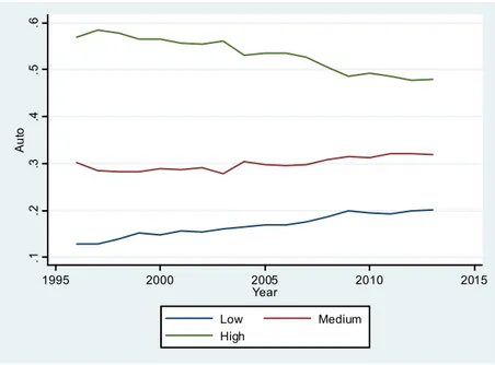
Figure 3.2 explores how the distribution of total employment changed over the period 1996-2013, dividing workers into three groups based on the estimated automation probabilities associated with a worker’s occupation (based on the 3-digit classification):
• The “Low” group contains workers in occupations with a Frey-Osborne automation proba-bility below 30 percent.
• The “Medium” group includes occupations with a Frey-Osborne automation probability above 30 percent but less than 70 percent.
• The “High” group contains occupations with a Frey-Osborne automation probability above 70 percent.
Figure 3.2 shows the development over time for workers in firms in the Swedish business sector with at least ten employees. The figure shows that the proportion of employment in the low-risk group has increased by approximately 7 percentage points. We also note that the share of jobs in the high-risk group decreased by approximately 9 percentage points, but most of this decline takes place in the period before 2009–after 2009, during the recovery from the financial crises, the share of employment with high-risk occupations levels out. Overall, Figure 3.2 indicates a shift in the disturbance of occupations in terms of exposure to automation. This is likely a result of the structural change in the Swedish labor market that started in the 1990s. Taken together, the pattern emerging from Figures 3.1 and 3.2 appears to show that overall employment in low-risk occupations declines–at least as a share of total employment.
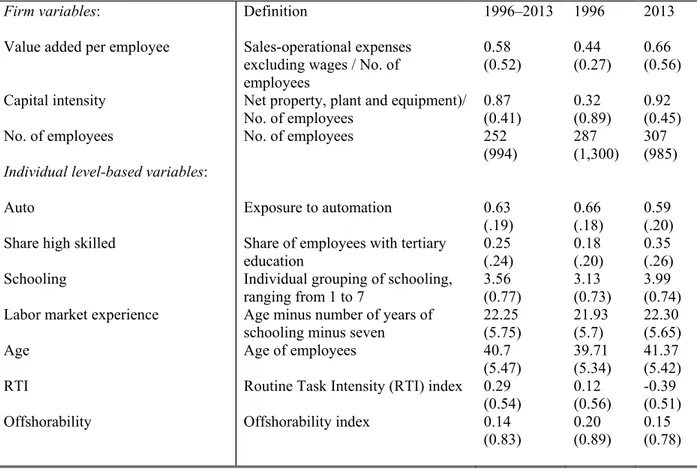
Finally, before presenting the econometric analysis, we present in Table 1 some descriptive statistics at the firm level on our data and variable definitions. From the table, we note that the pattern observed in Figure 3.2 above at the worker level can also be seen at the firm level. Our firm-level measure of exposure to automation decreased during our sample period, from a mean of 0.66 in 1996 to 0.59 in 2013. This implies that the workforce of Swedish firms has gradually changed towards occupations with less exposure to automation and is further evidence of a AI&R-driven structural change observed at the firm level. We can also see from Table 1 that there has been strong human capital upgrading, measured both in terms of the share of employees with university education and based on the mean schooling of individual workers. The table also presents firm-level
.1 .2 .3 .4 .5 .6 Au to 1995 2000 2005 2010 2015 Year Low Medium High
Figure 3.2: Employment shares in three groups based on automation probabilities, 1996-2013. measures of the routineness and offshorability of the workforce. Comparing 2013 with 1996, we note that firm-level means of both RTI (routine task intensity) and offshorability decreased during this period.5 Finally, we note that over the period 1996-2013, we observe an increase in both labor
productivity and capital intensity and a higher mean number of employees at the firm level. Table 1
3.2. Empirical specification
We will estimate the following specification:
log ( ) = + · + · _+ · _×
+ · log + · log() + + + (3.2)
The dependent variable in (3.2) is the log of value added per employee in firm at time log=
log(
), which is our measure of productivity.
6 Value added is calculated as the output value
minus the costs of purchased goods and services, excluding wages and other personnel costs. Our main variables of interest are which again denotes the workforce’s exposure to
automation in firm at time ; the share of skilled workers in the firm, _; and
the interaction _ × . The share of skilled workers is defined as the share
of employees with university education. We also control for the log of a firm’s capital intensity
5See Section 3.3.2 for details about these measures. 6
log() and log firm size log . All specifications include firm fixed effects, to control
for unobserved firm-level heterogeneity in productivity (i.e., the firm-specific demand and cost parameters in the model, and ) and year fixed effects that account for common shocks, .
Finally, is the error term. To allow for within-firm correlation over time, standard errors are
adjusted for clustering at the firm level. Let us now discuss expected signs of our main variables of interest in (3.2).
3.2.1. Testing Prediction 1
As discussed in Section 2.5.2, Proposition 2 and Equation (2.34) imply that a low skill share should be associated with laggard firms and how a higher skill share is associated with leading firms:7 In laggard firms, production employment increases when the return to investing in new technology increases, driving down the skill share; in leading firms, production employment declines when the return to investing in new technology increases, driving up the skill share. Using our variable , which measures how firms change their employment of workers susceptible to automation
together with the the share of skilled workers firms, _, we can use this information
to test Prediction 1 as follows.
First, differentiate (3.2) with respect to the workforce exposure to automation, to obtain:
log ( )
= + · _
(3.3)
In the limiting case of a laggard firm, we have lim _→0 µ log ( ) ¶ = (+) 0 | {z } "Laggard" (3.4)
In laggard firms–i.e., firms with a low skill intensity–increased (unobserved) investments in AI&R technology is associated with increased hirings of workers with a high risk of automation. Since investments in new technology increase productivity, productivity and work force exposure to au-tomation should be positively correlated, i.e., we expect 0 in (3.4).
7This can be formalized under the intuitive assumption that higher quality firm-specific assets associated with
higher consumer demand () and lower cost ()are related to more intense use of high-skilled non-production labor
in terms of the fixed number of non-production high-skilled workers, . More specifically, let = (
) 0with 0(
) 0. Let (
∈ (1 2)) denote the fixed number of non-production high-skilled workers in a laggard firm and let (
2)denote the fixed number of non-production high-skilled workers in a leading firm. Then, at = 0, if
( 2) ( ∈(12)) ∗ (0|2)
(0|∈(12)) holds, leading firms will always have strictly higher skill intensity than laggard firms, i.e., ∗(| 2) ∗(| ∈ (1 2)).
In the limiting case, for a leading firm, we have lim _→1 µ log ( ) ¶ = (+) + (−) 0 | {z } "Leader" (3.5)
In leading firms–i.e., firms with a high skill intensity–increased (unobserved) investments in AI&R technology also raise productivity, but in contrast this process now comes with fewer high-risk workers being employed. This will now cause productivity and work force exposure to automation to be negatively correlated, i.e., we expect 0 and + 0 in (3.5).
Given the estimates of 0 and 0, we can derive a cutoff to empirically distinguish the two firm types: Setting log()
= 0 in (3.3), we can find the skill share of a marginal firm,
˜
= − ∈ (0 1). We can get then classify firms with skill shares below ˜ as "laggard firms" (i.e.,
firms for which log()
0). And we can classify firms with skill shares above ˜ as "leading firms"
(i.e., firms for which log()
0)
3.2.2. Testing Prediction 2
We can also test Prediction 2 in a similar way. Differentiating (3.3) with respect to _,
we obtain
log ( )
_ = + ·
(3.6)
In the limiting case for a leading firm, we first have lim →0 µ log ( ) _ ¶ = (+) 0 | {z } "Leader" (3.7)
Again, in a leading firm, investments in AI&R technology raise productivity and reduce employment in high-risk jobs. Since the share of skilled workers and employment in high-risk jobs are negatively correlated (but not perfectly, as shown in the three panels of Figure 3.1), this will imply a positive correlation between the share of skilled workers and productivity, i.e., we predict that 0 in (3.7).
In the limiting case for a laggard firm, we finally obtain lim →1 µ log () _ ¶ = (+) + (−) 0 | {z } ”Laggard" (3.8)
Again, since investments in AI&R technology lead to increased productivity in tandem with the employment of workers who have a high risk of automation in laggard firms, the share of skilled workers will be negatively correlated with productivity, i.e., we predict that + 0 Setting
log( )
_ = 0 in (3.6) and solving for the marginal firm ˜ = −
identifying condition for firm types where firms with ˜ are considered as laggard firms,
and firms with ˜ are leading firms.
3.3. Empirical results 3.3.1. Benchmark results
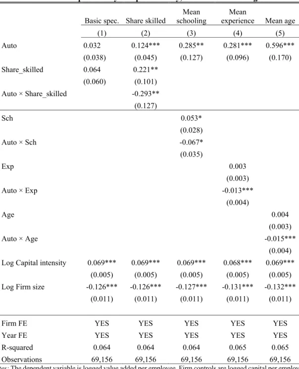
Let us start by estimating in (3.2) when excluding the interaction term, _× .
The results for this restricted model are shown in column one of Table 2. We find that the coefficient on the exposure to automation, is statistically insignificant. This may be expected since–as
shown by the theory–the relationship between exposure to automation and labor productivity should differ between firm types, and this heterogeneity is not accounted for when pooling firm types in a single relationship.
Table 2
In column two in Table 2, we turn to the results for the full specification in (3.2) which allows for firm heterogeneity. We find that the coefficient of , ˆ
, to be positive and statistically significant. The coefficient on the interaction with the skill share, _׈
, is negative and statistically significant. Substituting these estimated coefficients into (3.3), we obtain:
log³ ´ = ⎧ ⎪ ⎪ ⎨ ⎪ ⎪ ⎩ ˆ (+) + ˆ (−) · _ 0 if _∈ [0 042) ˆ (+) + ˆ (−) · _ 0 if _∈ (042 1] (3.9)
Expression (3.9) provides evidence for Prediction 1: Productivity as measured by value added per employee is increasing in the exposure to workforce automation when the share of skilled workers is low (i.e., when the skill share is less that 42%, i.e., ˜ = −ˆ
ˆ
= 042). However, productivity
declines when the exposure to workforce automation increases, namely, when the share of workers with tertiary education is sufficiently high (i.e., higher than 42%).
Recall the intuition behind these results: We imagine a process whereby–over time–AI&R technologies become increasingly available and more profitable. Investments in AI&R technology increase, but this is not observed in the data (see the top panels in Figure 2.2 and Figure 2.3). The AI&R technology causes productivity in all types of firms to rise. Since the output-expansion effect trumps the labor-replacement effect in laggard firms, employment of production workers susceptible to being replaced by the new technology increases. Therefore, investments in AI&R technology cause a positive correlation between labor productivity and high-risk production employment (see the middle and bottom panels in Figure 2.3). In contrast, in leading firms, the replacement effect dominates the output expansion effect, causing the employment of production workers susceptible to automation to decline. Investments in the AI&R technology then cause a negative correlation between labor productivity and production employment in leading firms (see the middle and bottom