Plant functional diversity across a spatial climate gradient in Sweden

(1)

Faculty of Natural Resources and Agricultural Sciences

Plant functional diversity across a spatial climate gradient in Sweden

Nina Lončarević

Master´s thesis • 30.0 credits

Independent project • Department of Ecology

Uppsala, Sweden 2019

(2)

Plant functional diversity across a spatial climate gradient in Sweden

Nina Lončarević

Supervisor: Alistair Auffret, Swedish University of Agricultural Sciences, Department of Ecology

Assistant supervisor: Frank Schurr, University of Hohenheim, Institute for landscape and plant ecology Examiner: Erik Öckinger, Swedish University of Agricultural Sciences, Department of Ecology

Credits: 30 hec Level: A2E

Course title: Master thesis in Biology

Course code: EX0895

Course coordinating department: Department of Aquatic Sciences and Assessment Place of publication: Uppsala, Sweden

Year of publication: 2019

Online publication: https://stud.epsilon.slu.se

Keywords: landscape ecology; plant functional ecology

Swedish University of Agricultural Sciences

Faculty of Natural Resources and Agricultural Sciences

(3)

Abstract

Introduction. Climate is a well-known and well-studied abiotic driver of the natural world working through e.g. physiological alterations in species, changes in species’ ranges and growing season, reduction in growth or causing mortality. Besides influencing vegetation zonation, climate is vital for plant functioning such as evapotranspiration, net primary productivity (NPP), nutrient cycling; as well as for vegetation structure, all of which are essential for ecosystem functioning and provisioning of ecosystem services to humans. Biodiversity is an important constituent of optimal ecosystem functioning and it is broadly accepted that diversity of plant functional traits, the characteristics of plants related to growth, dispersal, persistence, is what makes up ecosystem functioning and ecosystem response to environmental factors. Climate is often defined in terms of the mean and variability of atmospheric variables such as temperature and precipitation, which I will be using in my research.

Aims. The aim of my study is to investigate the effect of the Swedish spatial climatic gradient on plant functional diversity. I want to know how temperature and precipitation variation in Sweden affect a) functional richness (FRic; the richness of different plant functional traits within a community), b) species richness (number of species), c) community mean specific leaf area (SLA), d) community mean seed mass and e) community mean canopy height. Community trait means are mean values of functional traits in a given plant community or plot.

Methods. The data I used are species occurrence data (8193 unique species), functional trait data (13 functional traits), temperature, precipitation and land-use data across 6153 plant communities of 5x5 kmeach. Using them I performed a functional diversity analysis calculating FRic and community trait means, which I later analyzed with linear mixed models in R.

Results. Results for FRic indicate that in areas of high temperatures, the number of functional traits tends to be high, as well as in areas where high % forest cover and high temperatures. Species richness tends to be high in high temperature and precipitation areas, and low in areas with high forest cover and areas with high forest cover and precipitation. Seed mass is on average smaller in areas of increased temperature and precipitation. With high temperatures and % forest cover, seeds also tend to be smaller. Along the climate gradient in areas of higher temperature and precipitation, SLA tends to be larger. Likewise, in areas with more forest cover and higher temperatures, SLA is larger. In areas of high temperatures, canopy height was greater.

Discussion. My results show higher species richness and higher FRic in warmer areas across the present-day climate in Sweden. The functional traits examined (seed mass, SLA and canopy height) are all significantly affected by at least one and often both of the climate drivers. Additionally, as climate is undeniably changing, numerous species distributions and geographical range changes have been documented, as well as species extinctions and ecosystem functioning alterations. This leads to a possible and plausible conclusion that Swedish species and functional diversity will experience consequences of climate change. These changes are likely to have large implications for evolution of new suites of traits, unprecedented changes in ecosystem functioning and species gain in Sweden, as well as potential loss.

(4)

List of tables and figures

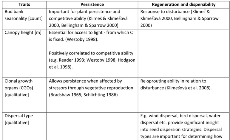
Table 1: All functional traits used in study and importance for plant functioning ... 7

Table 2: Core traits importance for ecosystem functioning, extracted from de Bello et al. 2010 ... 9

Table 3: AIC, conditional and marginal R squared and REML for FRic linear mixed model analysis ... 12

Table 4: Linear mixed model analysis for FRic ... 12

Table 5: AIC, conditional and marginal R squared and REML for species richness linear mixed model analysis ... 13

Table 6: Significant (+, -) and nonsignificant (ns) effects on climate and forest cover on response variables . 13 Table 7: AIC, conditional and marginal R squared and REML for seed mass linear mixed model analysis ... 14

Table 8: AIC, conditional and marginal R squared and REML for specific leaf area (SLA) linear mixed model analysis ... 15

Table 9: AIC, conditional and marginal R squared and REML for canopy height linear mixed model analysis 15 Figure 1: Effects on and effects of species traits (Chapin et al. 2005) ... 1

Figure 2: Swedish historical provinces for which species data was used in analysis ... 5

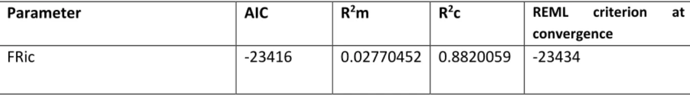
Figure 3: Effect of temperature and % forest cover interaction on functional richness ... 12

Figure 4: Effect temperature-precipitation interaction on species richness ... 13

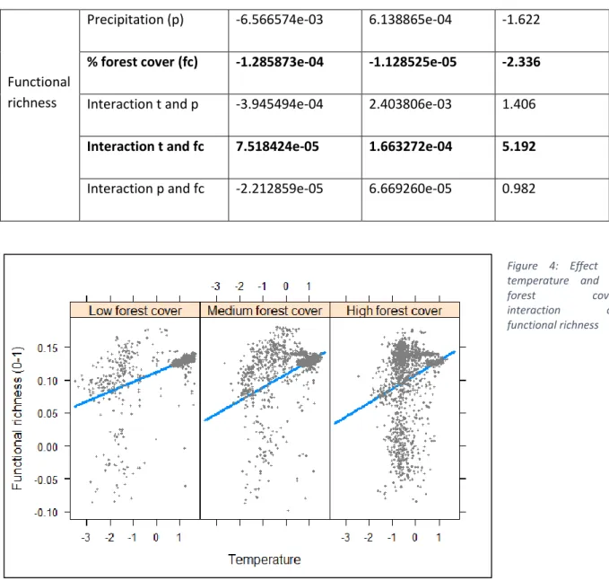
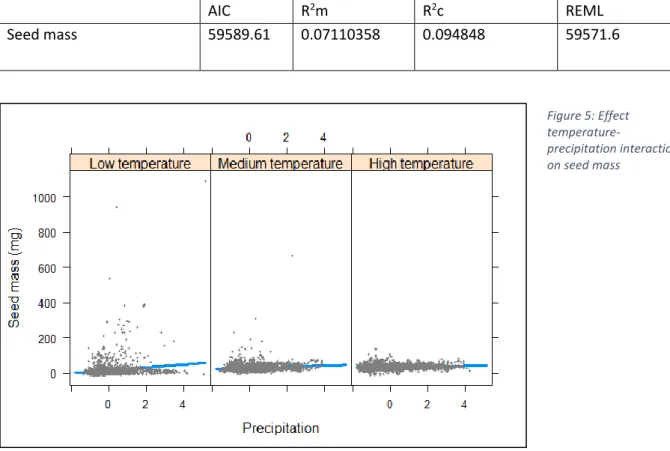
Figure 5: Effect temperature-precipitation interaction on seed mass ... 14

Figure 6: Effect temperature-precipitation interaction on SLA ... 15

(6)

1

Introduction

Climate is a well-known and well-studied abiotic driver of the natural world working through e.g. physiological alterations in species, changes in species geographical ranges and growing season, changes in vegetation zonation, reduction in growth or causing mortality. (Pigott & Huntley, 1981; Woodward, 1991) Climate is also vital for basic plant functioning such as evapotranspiration, net primary productivity (NPP), nutrient cycling; vegetation structure (vegetation height, distribution etc.). (Woodward, 1991) The classic example is dependence of plants on water, coming in great part from precipitation, for performing photosynthesis. It is of course not the only factor shaping vegetation structure and ecosystem functioning, climate is a part of a suite of abiotic and biotic drivers (geography, soil type etc.) which together influence the entire functioning of ecosystems. It represents a complex ecological gradient, often defined in terms of the mean and variability of atmospheric variables such as temperature, precipitation and wind. It can also be defined as a system, referring to the major factors influencing it: the atmosphere, the hydrosphere, the cryosphere, the land surface, the biosphere and the interactions between them. (Goosse H, et al 2010) In this research I focused on two major atmospheric climate components, temperature and precipitation.

In recent decades, climate change has become an issue influencing almost every aspect of society. It is defined as a change in weather patterns over a long period of time (Goosse H, et al 2010). The Earth's climate has warmed by approximately 0.6 – 0.8 °C over the past 100 years with two main periods of warming, between 1910 and 1945 and from 1976 onwards. The rate of warming during the latter period has been approximately double than that of the first and, therefore greater than at any other time during the last 1,000 years. (IPCC 2001). This is causing major biodiversity loss, geographical range shifts, onset of non-native species et cetera. (Thuiller et al 2005) Observed climate change is causing a major redistribution of European flora and fauna, with distribution changes of several hundred kilometers projected over the 21st century. (CNRS 2012) These impacts include northwards and uphill range shifts, as well as local and regional extinctions of species. What is more alarming are the species extinctions due to climate change which reduce global biodiversity levels, happening because species cannot keep pace with the changing climate, land use and other obstacles, shown on the example of birds and butterflies by CNRS 2012.

The loss of biodiversity strongly influences ecosystem functioning. Ecosystem functioning in colloquial language encompasses various terms, including ecosystem properties, ecosystem goods and ecosystem services (the latter two often used interchangeably), hence the need to define each, as they will be used here. Ecosystem properties include the abiotic and biotic structures and processes of ecosystems like soil properties, biomass production, nutrient cycling and many others, which are the ‘’makers’’ of ecosystem services and form the basis for societal development. (Bastian, Haase, Grunewald 2012) Ecosystem services are the benefits people obtain from ecosystems, directly through market-value based ecosystem goods such as food, construction materials, medicines, or indirectly through maintenance of hydrologic cycles, regulation of climate, cleansing of air and water, maintenance atmospheric composition, pollination, soil genesis, storage and cycling of nutrients etc. (Ma, M. E. A., 2005) Although varying in terms of levels, rates, or amounts, none of ecosystem properties performance are inherently ‘‘good’’ or ‘‘bad’’. On the contrary, ecosystem services do carry the labels ‘’good’’ and ‘’bad’’, given to them by humans who are directly dependent on them and attach value to them. (Chapin et al. 2005) Many ecosystem services are being exploited in a

(7)

non-2 sustainable fashion or degraded, which includes fresh water provision, air and water purification, regulation of pests and local climate and so on. (Ma, M. E. A., 2005).

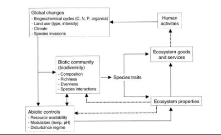
Ecosystem functioning is inseparable and highly reliant on biodiversity, explored by a specific research field, biodiversity-ecosystem functioning (BEF), particularly within the study of ecosystem services. (Schröter 2019) To be clear, biodiversity encompasses a broad categorization of richness and distinctiveness of biological life on Earth, including diversity of genotypes, traits, species, ecosystems, biomes, landscapes etc. (Gaston 1996, Purvis and Hector 2000) For instance, as shown by Reich et al. (2001), plant biodiversity enhances ecosystem productivity. In their experiment they found that 16-species mixtures contribute more on average to biomass generation than monocultures and 4 or 9 species mixtures in enhanced CO2 and N deposition treatments. They established that 4 species were dominant in biomass production in the 16-species mixtures, however, these same species planted as monocultures under the same resources produced lower biomass on average. Two decades of BEF research are congruent with this and present biodiversity importance for pollination, pest control, carbon storage et cetera. (Tilman et al. 1997, Loreau & Hector 2001) Moreover, ecosystem functioning and biodiversity have large repercussions for ecosystem service provision to humans which are especially under threat due to the changing climate of the past decades. For example, as runoff to lakes and streams is becoming a major issue in urbanized areas, introduction of a deep-rooted species into Mediterranean ecosystems allows them to access previously inaccessible water and nutrient sources and act as an important buffer for runoff or in recovery of degraded ecosystems. (Chapin III et al. 1997). Hence, determining patterns behind biodiversity from community to ecosystem scale is important for understanding how is ecosystem service provision changing and how can we adapt to it in a way that conserves biodiversity and ecosystems and satisfies human needs. (Diaz et al. 2006) Looking at biodiversity into even more depth in connection to ecosystem functioning, it is broadly accepted that diversity of functional traits makes up ecosystem functioning as well as ecosystem response to environmental factors. (Figure 1) (Lavorel and Garnier 2002) Following Darwin's (1859) proposal, traits were initially mainly used as predictors (proxies) of organismal performance. Over the last three decades, developments in community (Grime 1974, Petchey and Gaston 2002) and ecosystem (Chapin III 1993, Lavorel and Gamier 2002) ecology have moved the concept of trait beyond these original boundaries, and trait-based approaches are now used in studies ranging from the level of organisms to that of ecosystems. In my research I followed a definition from Perez-Harguindeguy et al. 2016 ‘’functional traits to be

any morphological,

physiological or phenological feature, measurable for individual plants, at the cell to the whole-organism level, which potentially affects its fitness (McGill et al. 2006; Lavorel et al. 2007) or its environment (Lavorel and Garnier 2002).’’ This places

Figure 1: Effects on and effects of species traits (Chapin et al. 2005)

(8)

3 functional traits ‘’in medias res’’ i.e. in the midst of ecosystem functioning by being foundation for ecosystem responses to environmental changes (disturbance, climate, resource limitations etc.) and building blocks of ecosystem properties (Dıaz and Cabido 2001; Lavorel and Garnier 2002; Suding et al. 2008). Based on this fundamental distinction, functional traits can be split into response traits and effect traits. It is easiest to look at functional traits as forming a cycle: response traits direct how a community responds to environmental change, the changed community affects ecosystem processes through effect traits. (Suding et al. 2008) An example of this cycle are response traits specific leaf area (SLA) and leaf nitrogen content (LNC) which in response to nutrient and water availability construct effect traits leaf area and leaf mass. These traits then affect leaf palatability and leaf decomposability which are components of ecosystem functioning, perceived on a large scale. (Diaz et al. 2004) There are some traits which are simultaneously response and effect traits, an example are traits both responding to land use change in European grasslands and affecting nutrient cycling (Garnier et al., 2004) Examples of response traits are seed size, important for regeneration capacity under different disturbance regimes, bark thickness, related to fire tolerance, leaf size which causes different heat balances to name a few. (Diaz et al. 2013 and references therein) Examples of effect traits are water retention capacity in bryophytes which regulates ecosystem hydrology, leaf N content in vascular plants which accelerates the nutrient cycling rate etc. (Diaz et al. 2013 and references therein) The structuring of biological communities depends on how successfully they go through selective filters of ecological gradients - climate, disturbance, resources (Keddy 1992), site productivity (Woodward & Diament 1991), to name a few. They act as a funnel i.e. traits first have to be adept to climatic conditions, then to the dominating disturbance regime and so on (Diaz and Casanoves 1998), and this has large implications over evolutionary time. In the complexity of abiotic and biotic drivers of community composition and biodiversity (Figure 1), climate is possibly the largest threat to species and ecosystem functioning. Since change of community composition over time is difficult to study due to a lack of historical data, spatial gradients can be a useful way to look at the effect of climate on diversity, composition, functional traits etc. Other than a profound interest of community ecology in the study of functional traits (Raunkiaer 1934, Grime 1977) their undeniable impact on biodiversity and ecosystem functioning (Schulze and Mooney 2012, Schröter 2019), the study of climate affecting functional diversity is also important as a stepping stone to enabling predictions of the impact of climate change on functional processes.

The aim of my study is to investigate the effect of the Swedish spatial climate gradient on plant functional diversity. Specifically, I want to know how temperature and precipitation variation in Sweden affects: a) functional richness (FRic), b) species richness, c) community mean seed mass, d) community mean specific leaf area (SLA) and e) community mean canopy height. Community trait mean is the average value of a trait in a plant community taken from individual traits of plants measured. Additionally, I include land use in the research. It is not the focus in my study, hence I include it as a proxy variable, % forest cover, since it is an important predictor of functional diversity and trait variation. I wanted to examine temperature and precipitation effects because they, as climate factors, are ranked highest among drivers of terrestrial ecosystem change and vegetation zonation which is also true of land use (Sala et al. 2000, Woodward et al. 2004). In a similar study, Vanneste et al. 2019 studied the role of monthly temperature, precipitation extremes and patch-scale factors in shaping the functional trait distribution of understory herbs. They found that the environmental variables explained on average 77% of the variation in community trait means. Similarly, Wieczynski et al 2019, in their research about climate shaping functional biodiversity in forests, found climate strongly

(9)

4 governs functional diversity with temperature variability and vapor pressure being the strongest drivers of geographic shifts in functional composition. Functional richness and species richness are highly correlated because of the assumption that higher species richness leads to higher functional richness, (Petchey and Gaston 2002), however they are not surrogate (Diaz and Cabido 2001) and it is commonplace that they are studied separately. Species richness is well-known to increase towards the equator (Brown 2014) due to historical and ecological reasons such as increase of optimal plant conditions. I expect to see higher species richness in areas of higher temperature and precipitation in Sweden, since the increase of optimality of environmental conditions is mainly southward. I also expect to see a rise in species richness and functional richness with % forest cover. Swedish forests are mostly monocultures or mixed stands of two tree species (Swedish National Forest Inventory 2019, Felton et al. 2016) so I do not expect high tree diversity but diversity of lower canopy species (Gilliam 2007). I expect canopy height (equivalent to plant height) to increase with availability of resources i.e. increased temperature and precipitation across the climate gradient (Moles et al. 2009). For seed size it is suggested that higher temperatures might result in higher metabolic costs of seedling growth and hence select for larger seed size (Lord et al. 1997), hence I expect an increase in seed mass with temperature and precipitation. For specific leaf area (SLA) I also expect an increase with temperature and precipitation due to resource-rich conditions, as shown by Anacker et al. 2011 who investigated how climate, soil, and fire drive community-level variation in SLA. They found that SLA was consistently high, regardless of the other variables, in mesic coastal climates (high temperature and precipitation). I expect forest cover to affect seed mass negatively i.e. seed mass to be lower in areas of higher forest cover, since due to heterogeneity in forests and often fragmentation, smaller seeds have a higher probability of getting dispersed (Silva and Tabarelli, 2000, Tabarelli and Peres, 2002). I expect an increase of SLA in forests to optimize the surface for light capture due to light competition in forests, possibly selecting for higher SLA (Givnish 1988) and possibly higher canopy height in forests due to the same reason of light competition (Westboy et al 1998).

Methods

Study area

Sweden is a country in northern Europe, bordering the Baltic Sea, Gulf of Bothnia, Kattegat and Skagerrak seas, Finland and Norway. It has mostly flat terrain or gently steep lowlands with high mountains in the west. Mean elevation is 320 m, while highest elevation point is near Kristianstad, 2111m (Kebnekaise). Most of Sweden is forested (68%), with small parts of cropland mainly in the south (7.5%). The country has almost 100 000 lakes, the largest of which, Vänern, is the third largest in Europe (Central Intelligence Agency, ed. 2007). Sweden administratively comprises of 21 counties, while it also has historical provinces (25), although not of official use. Although it is popular belief cold harsh weather is present everywhere in Sweden for most of the year, this is not particularly true because of the inflow of mild air from the Atlantic Ocean (Gulf stream) which makes the climate milder. The Swedish climate is highly seasonal and depending on the region, spring runs from March/April to May, summer from June to August, fall from September to October/November and winter from November/December to March/February (Sweden.se, 2018). A distinct feature of Swedish summer is that along the entire coast of the Baltic sea there is equal temperature distribution with hardly any decrease northwards during the warmest month, July (15-17 °C). As one goes inland, the temperatures decrease with altitude, coming to around 10-11 °C during July in Swedish mountains. Due to the strong south-north temperature shifts in spring and autumn, there is a significant difference in climate

(10)

5 zonation and thus in the length of the growing season. In southern Sweden, snowfall is often erratic but rain more frequent, without lasting snow cover formation. In central Sweden the snow cover lasts on an average 4-5 months while in the north snowfall is more regular, often occurring from October to April. (Central Intelligence Agency, ed. 2007)

Thanks to Sweden’s length, 1,574 km (Central Intelligence Agency, ed. 2007), the country has significant climatic variety and also distinctive vegetation zonation. Swedish vegetation zones encompass 4 categories, namely: 1) The nemoral (temperate) zone - the southern deciduous forest region. This region has the richest flora of entire Sweden with regard both to remnants of semi-natural vegetation in forests, woodlands and former grazing grounds and to the borders of agricultural fields; 2) The boreo-nemoral (hemi-boreal) zone is sometimes referred to as the southern coniferous forest region, with pine and spruce dominating. There are some differences within the zone, not only due to altitude and latitude, but also due to a west-to-east gradient; 3) The boreal zone is the northern coniferous forest or taiga region and includes the vast area up to the forest limit in the mountains. It is common to divide it into three subzones: the southern, the middle and the northern one; 4) The alpine zone, above the forest limit, is conventionally divided into three vertical belts, the low alpine, middle alpine and high alpine. (Rydin 1999)

Data

The data I use are species occurrence data, functional trait data, climate (temperature and precipitation) and land-use data. Preparation of all data and the statistical analysis were done using R software (R Core Team 2017) and R Studio (RStudio Team 2015). Additionally, all the data was gridded on a 5x5 km grid to represent plant communities for the purpose of calculating community means of functional traits, species richness and functional richness, explained further in the Data analysis. The two terms, grid squares and plant communities, will be used interchangeably.

Species occurrence data

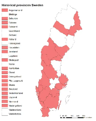
The species occurrence data was obtained from provincial plant atlases. This was done mostly via the Species Observation System (Artportalen 2018), an online species-observation tool whose contributors are, on an ongoing basis, individuals, NGOs, private institutions or other authorities. An observation in the data base includes species identity, location, date, square grid of observation (since the data is gridded on a 5x5 km grid) but also information such as habitat type and weather. This database is the

Figure 3: Swedish historical provinces for which species data was used in analysis

(11)

6 main source of species occurrence data for Swedish local authorities, Swedish Forest Agency (Skogsstyrelsen), Swedish Transport Administration (Trafikverket) etc., making it more than suitable for use in this instance. The data was obtained in 2019 by A.G. Auffret for all historical provinces (18 out of 25) which have an ongoing or recently-published plant biodiversity atlas for which data are available. To be clear, Swedish provinces are different from Swedish counties. Provinces refer to historical administrative units while counties are present-day administrative units and official within-country boundaries. Occurrence records for each atlas were generally collected across two decades, with the entire data set including records from 1975 until 2018. Data were then cleaned of obvious errors and observations were assigned to the 5x5 km grid that is used for the majority of atlas projects. After receiving these data, I constructed 18 data frames for each individual province with information on presence/absence of each species for each grid square, using the R package mefa (Peter Solymos 2009). These are also called species x species matrices and they were used later in the calculation of functional diversity (FD) indices. The total number of unique species is 8193.

Functional trait data

For functional traits I chose 13 life-history traits from the LEDA database (Kleyer et al. 2008), which specializes in Northwest European flora. The LEDA database is a project initiated by European Commission (EC) within the Energy, Environment and Sustainable Development program (EESD), aiming to provide an open source database of plant traits. The database was built relying on existing databases, literature compilations, unpublished data from project participants and additional measurements. All data must have included referenced literature (if the data is compiled in such a way), or other than that a geographical reference, EUNIS habitat classification codes and habitat characteristics, soil type, management type and method of measurement whenever possible to be included. The database mostly aggregated ‘’soft traits’’ i.e. easy to measure traits that are (often in combination) good indicators of plant functions. For example, specific leaf area (SLA) is an easily measured soft trait that may serve as a good indicator of growth rate, which is a ‘’hard trait’’ i.e. complex plant function (Diaz et al. 2004).

My research does not target a specific trait, plant organ or plant function (e.g. dispersibility), which is why I choose a broad scope of functional traits to observe their response to spatial climatic variation. My choice was guided as to include key features of plant dynamics: persistence, regeneration and dispersibility. Plant dispersibility is seed transport away from a parent plant. It is important for reducing the risk of distance- or density-dependent mortality, for regeneration after disturbance, colonization of new habitat etc. (Kleyer et al. 2008). Plant persistence is the ability of a plant to survive and thrive in an environment and plant regeneration is physiological renewal, repair, or replacement of tissue in plants (commonly after a disturbance). (Begon et al. 2006) In these three categories I included a) traits considered relevant almost globally due to their role in the plant life cycle (Grime et al. 1997; Weiher et al. 1999) and b) traits evidenced as important in ecosystem functioning and as responses to climate, matched with availability of data in LEDA (Table 1). Belonging to group are a) seed size (expressed in my research as seed mass), structure of leaf tissue (expressed in my research as specific leaf area (SLA)) and plant height (commonly expressed as plant size) instead of which I used canopy height, introduced by Westoby 1998 and supported by Weiher et al. (1999) as a ‘’top 3’’ important trait. De Bello et al. (2010) with references therein gives a good overview of which ecosystem processes these traits support (Table 2). Besides these three core traits, for construction of species x traits matrices for calculation of functional richness, species richness and community mean traits, I chose:

(12)

7 plant lifespan, dispersal type, seed mass, shoot growth form, buds seasonality, clonal growth organs, leaf distribution, leaf mass, leaf size and releasing height (seed), leaf matter dry content (lmdc). This is detailed in the section Functional diversity data of the Methods. This choice is also supported by a paper presenting a list of plant traits for functional ecology Weiher et al. (1999), the ‘’common core list’’, as a starting point for research in functional ecology and it includes seed mass, seed shape, dispersal mode, clonality, specific leaf area (SLA), leaf water content, height, aboveground biomass, life history, onset of flowering, stem density, and re-sprouting ability. Some of these traits are hard traits and are nowadays commonly represented as a measure of several soft traits.

To construct traits x species matrices needed in the FD analysis, first I constructed a dataset of all unique Swedish species from 18 provinces and all traits from 13 data sets. The trait datasets obtained from LEDA were not complete for many traits and I used a recommended method (Taugourdeau et al. 2004) - mice package (Stef van Buuren 2011) in R to perform an imputation of the missing data. It offers different method to deal with missingness in a dataset. It works in a way to create multiple replacement values (imputations) for multivariate missing data, including continuous, binary, unordered categorical and ordered categorical data. The method is based on Fully Conditional Specification, where each incomplete variable is imputed by a separate model. The imputation method I used was cart (Classification and regression trees), and relied on the default imputation number (5). The amount of missing data was around 30 %. After merging all trait datasets, I removed species not present in LEDA trait database and the resulting dataset (in further text all traits dataset) consisted of 8193 unique species. I then merged, individually, each of the 18 species occurrence datasets with the all traits dataset, where for each of them I kept trait information but erased any species that did not have trait information for at least one of the traits. This gave me 18 difference species x traits matrices.

Table 1: All functional traits used in study and importance for plant functioning

Traits Persistence Regeneration and dispersibility

Bud bank

seasonality [count]

Important for plant persistence and competitive ability (Klimeš & Klimešová 2000, Bellingham & Sparrow 2000)

Response to disturbance (Klimeš & Klimešová 2000, Bellingham & Sparrow 2000)

Canopy height [m] Essential for access to light - from which C is fixed. (Westoby 1998).

Positively correlated to competitive ability (e.g. Reader 1993; Westoby 1998; Hodgson et al. 1998).

Clonal growth organs (CGOs) [qualitative]

Allows persistence when affected by stressors through vegetative reproduction (Bradshaw 1965; Schlichting 1986)

Re-sprouting ability in relation to disturbance (Klimešová et al. 2008).

Dispersal type [qualitative]

E.g. wind dispersal, bird dispersal, water dispersal etc. provide significant insight into seed dispersion strategies. Dispersal types are important for determining how

(13)

8 far species disperse, randomly directed, but still relevant for quantifying

establishment of species and colonization (Weiher et al. 1999)

Leaf distribution (canopy

architecture) [qualitative]

Helps measure light interception and light access of plants, critical to plant growth (e.g. Horn 1971, Niinemets 2010)

Leaf mass [mg] Important for quantifying photosynthesis, essential for plant vitality. (Meng, Cao, Yang 2013)

Important for quantifying light access (with other co-varying leaf traits) (Meng, Cao, Yang 2013, Niinemets 2010)

Leaf size [mm^2] Important for quantifying photosynthesis, essential for plant vitality. Meng, Cao, Yang 2013, Weiher et al. 1999)

Leaf matter dry content (lmdc) [mg/g]

Important for quantifying photosynthesis, essential for plant vitality. (Meng, Cao, Yang 2013)

Conservation of nutrients (low SLA, high LDMC) (Garnier et al. 2001b)

Plant lifespan [qualitative]

Annuals, bi-annuals, perennials: can explain why species persist in a certain environment where they don’t reproduce (Weiher et al. 1999)

Seed mass [mg] Critical for seedling establishment and important when competition is a factor (Reader 1993; Leishman & Westoby 1994; Osunkoya et al. 1994)

Important for seed longevity. (Leishman & Westoby 1998, Weiher et al 1999)

Regeneration: fecundity, seedling establishment, dispersal (Fenner 2010) Seed mass is a good proxy of temporal dispersal because generally, small seeds can travel further (Reader 1993; Leishman & Westoby 1994)

(14)

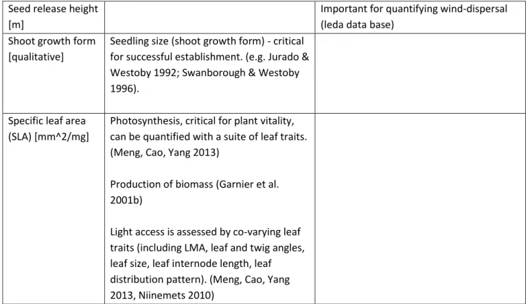
9 Seed release height

[m]

Important for quantifying wind-dispersal (leda data base)

Shoot growth form [qualitative]

Seedling size (shoot growth form) - critical for successful establishment. (e.g. Jurado & Westoby 1992; Swanborough & Westoby 1996).

Specific leaf area (SLA) [mm^2/mg]

Photosynthesis, critical for plant vitality, can be quantified with a suite of leaf traits. (Meng, Cao, Yang 2013)

Production of biomass (Garnier et al. 2001b)

Light access is assessed by co-varying leaf traits (including LMA, leaf and twig angles, leaf size, leaf internode length, leaf distribution pattern). (Meng, Cao, Yang 2013, Niinemets 2010)

Table 2: Core traits importance for ecosystem functioning, extracted from de Bello et al. 2010

Core traits and ecosystem functioning

Canopy height Seed mass Specific leaf area (SLA)

Evapotranspiration; Infiltration/ maintenance of soil humidity; Surface water flow/ run-off; Carbon sequestration in vegetation and soil; Heat exchange; Erosion prevention; Permafrost insulation; Hurricanes/wind damage

resistance; Accumulation of standing biomass

Ecosystems dynamic and restoration

Decomposition and mineralization, nutrient mobilization;

evapotranspiration; Infiltration/ maintenance of soil humidity; Nutrient/sediment retention; Herbivory control; Fire risk prevention; Accumulation of standing biomass

Climate data

Climate data was obtained from Swedish Meteorological and Hydrological Institute’s 4 km gridded climate data from 1961-2011

(

SMHI 2019), as separate temperature and precipitation datasets with information on monthly mean precipitation and temperature for each grid. The data is collected from meteorological stations in the country and interpolated. Since the data on species occurrence is gridded on a 5x5 km grid, I had to harmonize it with climate data to perform the analysis. I did this by merging the 5x5 km grid square with, separately, temperature and precipitation data, and the result was a yearly mean for each grid square and each year. Furthermore, the species occurrence data are from various year spans, hence I needed to determine a consistent climate data span, and I opted for

(15)

10 1990 – 2011, across all provinces. To perform the analysis, I calculated a mean value of this year-span for each grid square.

Land use data

Land use analysis was not the primary focus of the research but I accounted for land use through a proxy - % forest cover since. Forest cover is important in a given ecosystem because it helps regulate the hydrological cycles, soil conservation, climate change, and, to a lesser degree biodiversity loss (Rudel et al 2005), Forest cover can also affect how macroclimate relates to the microclimate (Frenne et al 2019). The land use data was obtained from Environmental protection Agency of Sweden (Swedish Environment Protection Agency 2019) as a single raster file for entire Sweden. The base layer I downloaded is created from satellite data, information from laser scanning and to a lesser extent, with the aid of existing map data. The land cover data is mapped into 25 thematic classes. The mapping is in raster format with a resolution of 10 meters and with a smallest mapping unit down to 0.01 hectares. I performed the same process of harmonization with species occurrence 5x5 km grid. Out of the 25 thematic classes, I removed the marine water thematic class. I created the % forest cover proxy by combining forest-related thematic classes, in total 12 of them, and calculated their percentage in the total sum of thematic classes for each plant community i.e. 5x5 km square. I will use the term % forest cover in further text.

Functional diversity indices calculation

To perform the analysis of climate and % forest cover on traits and functional richness (FRic), I had to calculate FRic and species richness per each plant community as well as plant community trait means for seed mass, SLA and canopy height. Community mean is the dominating trait value of a given trait all species in a plant community, different from community-weighted mean which also takes into account species abundances. Ideally computation of community means includes abundance since it affects functional trait composition, this data is hard to obtain for a large-scale study such as this one and presence/absence data suffices. (Mason & Mouillot 2008, Diaz 2007) There have been many functional diversity (FD) indices proposed, summarized nicely by Mouchet et al. 2010. They divide the FD indices into three major groups necessary for describing FD: functional richness, functional evenness and functional divergence. The main index I focus on in my research is functional richness (FRic) which is, as described by Villéger, Mason & Mouillot (2008), the amount of functional space occupied by a species group and calculated as convex hull volume of functional space occupied by species. The computation of functional evenness (FE) and functional divergence (FDvg) is more heavily reliant upon abundance data, which were not possible to obtain from the plant atlas data used in this study, and could therefore not be calculated.

The calculation of indicated metrices was done with FD package (Laliberté 2014) in R. The necessary datasets for calculation, 18 traits x species matrices (x) and 18 species abundance matrices (a) (or presence-absence matrices in my case) for each province, were prepared as described previously. The result were 18 datasets for 18 different historical provinces with information on FRic, number of species and community means of traits for each plant community. They were then merged in one dataset (FD dataset in further text). Temperature, precipitation and % forest cover data were constructed in a way to contain a single value per plant community, and they were then merged with the FD dataset. There were 300 plant communities for which there was no land-use data, and these were therefore removed prior to analysis. I additionally erased plant communities (5x5 km squares)

(16)

11 with less than 25 different species since it is highly unlikely that a plant community would contain so few species. The number 25 was chosen arbitrarily, aiming for a good measure of minimum species richness per one plant community of indicated size. Additionally, the number of plant communities went down from 11 543 to 9859 when removing these grid squares. I also removed grid squares with more than 50 % inland water in them and this resulted in total of 6153 grid squares finally used in the analysis. The inland-water grid squares with more than 50% water in them were removed to increase accuracy of analysis by using landscape that is dominantly terrestrial, since I am looking at terrestrial plant communities.

Data analysis

I tested the relationship between climate and land use using a linear mixed model from the lme4 package (Bates et al. 2015). In total I did 5 lmer analyses, where response variables were, individually, FRic, species richness, community mean seed mass, community mean SLA and community mean canopy height. As explanatory variables for all 5 models I used temperature, precipitation and % forest cover and their two-way interaction, as well as region (18 different historical Swedish provinces) as a random effect. Temperature and precipitation explanatory variables were standardized with the scale function in R, which is a data-preparation process which centers chosen data around 0 and scales with respect to the standard deviation. (Brown-Anderson 2016) This is used since these variables have different units of measurement and are incomparable otherwise and not useful for the statistical analysis. I also calculated confidence intervals for each of the 5 models. I log transformed SLA because of right skew in the data, however this method did not prove to be relevant for other models. To visualize the results of the lmer analyses I used R package visreg (Breheny 2017), as it proved handy in presenting the interaction effects and non-interaction effects in a neat way.

Results

Main results – Functional richness

Significant positive effects on FRic have had temperature and the interaction of temperature and % forest cover, while negative effects have precipitation and % forest cover, individually. (Table 4) This indicates that in areas of high temperatures, the number of functional traits present in a plant community tends to be higher, as well as in areas with high % forest cover and high temperatures (Figure 3). On the other hand, with higher % forest cover there is a decrease in functional richness, which is true for areas of abundant precipitation too.

Table 3: AIC, conditional and marginal R squared and REML for FRic linear mixed model analysis

Table 4: Linear mixed model analysis for functional richness (FRic)

Parameter Fixed effects lower-95 upper-95 T value

Temperature (t) 4.974608e-03 1.469323e-02 3.974

Parameter AIC R2_m _R2_c _REML _criterion _at

convergence

(17)

12 Functional

richness

Precipitation (p) -6.566574e-03 6.138865e-04 -1.622

% forest cover (fc) -1.285873e-04 -1.128525e-05 -2.336

Interaction t and p -3.945494e-04 2.403806e-03 1.406

Interaction t and fc 7.518424e-05 1.663272e-04 5.192

Interaction p and fc -2.212859e-05 6.669260e-05 0.982

Main results – species richness

A significant effect on species richness have temperature (positive), precipitation (negative), their interaction (positive), % forest cover (negative) and interaction of % forest cover and precipitation (negative) (Table 6; Appendix 1). The interaction results indicate that across the climatic gradient, there is a significant increase in species richness with higher temperatures, regardless of the precipitation conditions (low, medium and high). (Figure 4). Higher % forest cover yields lower species richness, and areas with high % forest cover and high precipitation levels, species richness is also lower.

AIC R2_m _R2_c _REML Species richness 59589.61 0.09850255 0.7050792 59571.6 Figure 4: Effect of temperature and % forest cover interaction on functional richness

(18)

13

Table 6: Significant (+, -) and nonsignificant (ns) effects on climate and forest cover on response variables

Main results – Seed mass

A significant positive effect on seed mass have temperature and precipitation, their interaction (negative), % forest cover (positive) and interaction of temperature and % forest cover (negative) (Table 6; Appendix 1). In low temperature areas, higher seed mass with higher precipitation is observable, while this trend is negative for medium and high temperatures, where seeds tend to be smaller with precipitation, resulting in an overall negative interaction effect. (Figure 5) This indicates seeds tend to be smaller in areas of increased temperature and precipitation. The individual effects of these variables show the opposite: seeds tend to be larger in areas of high temperature and areas of high precipitation. In areas of higher temperatures and % forest cover, seeds tend to be smaller, while individual effects of these environmental variables also show the opposite i.e. seeds are larger with more forest cover, and also with higher temperature, as stated previously.

Model FRic Sp richness Seed mass SLA Canopy height

Temp + + + ns + Prec - + + ns ns % forest cover - - + ns ns Temp + prec ns + - + ns Temp + fc + ns - + ns Prec + fc ns - ns ns ns

Figure 4: Effect temperature-precipitation interaction on species richness

(19)

14

Table 7: AIC, conditional and marginal R squared and REML for seed mass linear mixed model analysis

AIC R2_m _R2_c _REML

Seed mass 59589.61 0.07110358 0.094848 59571.6

Main results – Specific leaf area (SLA)

The model for SLA showed significant positive effects for interactions of temperature and precipitation and interaction of temperature and % forest cover (Table 6; Appendix 1). Along the climate gradient in areas of higher temperature and precipitation, SLA tends to be larger (Figure 6). Likewise, in areas with more forest cover and higher temperatures, SLA is also higher.

Figure 5: Effect temperature-precipitation interaction on seed mass Figure 6: Effect temperature-precipitation interaction on SLA

(20)

15

Table 8: AIC, conditional and marginal R squared and REML for SLA linear mixed model analysis

Main results – canopy height

For canopy height, only temperature had significant positive effect on its increase (Table 6; Appendix 1) i.e. in areas of high temperatures, canopy height is greater. (Figure 7)

Table 9: AIC, conditional and marginal R squared and REML for canopy height linear mixed model analysis

Discussion

Climate is one major driver of species, biomes and functional trait distributions (Woodward, 1987). I apply this premise to assess the potential impact of climate on functional richness of plant species occurring in Sweden, species richness and functional traits (seed mass, SLA and canopy height). My main aim with this study was to see how they vary with the spatial climate gradient of Sweden. Additionally, I will discuss and draw provisional conclusions on possible climate change effects. My results confirm theory and previous findings, adding to and confirming the knowledge of climate impact on functional richness and species richness.

Functional richness

SLA (log transformed) -21239.42 0.04157437 0.1088863 -21257.4

Canopy height 6944.835 0.1077177 0.1649121 6926.8

Figure 7: Effect temperature on canopy height

(21)

16 The overall trend of FRic increase in areas of high temperature and precipitation is consistent with previous findings (Mason et al. 2003, Wieczynski et al. 2019), following the assumption that harsh environments decrease functional diversity and select for a narrow range of conservative growth strategies. (Zanne et al. 2014, Anderson et al. 2011) This is also in line with patterns observed by Cornwell and Ackerly (2009), which stated that regions with harsh environmental conditions are expected to have lower FD compared to regions with favorable conditions and with plant communities with stronger competitive interactions. Greater range in tree sizes and heterogenous forest understory, typical for old growth forests and low management regimes, contribute to increased functional diversity (Wilson and Peter 1988), which is the opposite case for most of Swedish forestry (Felton et al. 2016, Axelsson 2007) and possible explanation of decrease of FRic in areas of high % forest cover. However, the interaction of % forest cover and temperature indicates FRic is higher in areas with a lot of forest cover and higher temperatures, potentially indicating that temperature has a strong effect on FRic since its effect prevailed in the interaction.

Species richness

Increase of species richness with milder climate was expected and based on one of the oldest principles in biogeography - latitudinal diversity gradient (LDG). (Pianka 1966) This theory states that species richness increases towards the equator with decreasing latitude, and do so due to historical and ecological reasons, the latter being in this case increase of temperature and precipitation (Brown 2013). Decrease of species richness in areas of higher % forest cover does not match my expectations, since forests are overall biodiverse ecosystems, in large as a function of herb-layer community diversity (Gilliam 2007). This is potentially due to the fact that Swedish forests are heavily managed systems for wood production with very little virgin forest left which hence affects biodiversity of the lower canopy, besides the tree stands themselves being mainly mono cultures or mixed stands of 2-3 species (Swedish National Forest Inventory 2019, Hemström et al. 2014). In areas with high % forest cover and high precipitation levels, species richness is lower, possibly indicating a strong and prevailing effect of forest cover on species richness, since precipitation is well-known as an environmental factor increasing species richness (Gentry and Dodson 1987).

Seed mass

All explanatory variables for seed mass analysis (% forest cover, temperature and precipitation) have a positive effect on seed mass, while interaction of temperature and precipitation and interaction of temperature and % forest cover both having a negative effect. Seed mass increase with temperature and precipitation individually is expected (Moles et al 2003, Silvestre et al. 2019), since these are essential for seeds embryo development which is a predecessor of seedling and then grown plant. (Copeland and McDonald 1936). Larger seed mass in areas with more % forest cover was unexpected. To stablish successfully, plants are best of if their seeds are dispersed further away from the source to avoid competition with the mother plant (Leishman & Westoby 1994), making lighter seeds which then disperse easier. Dispersal is in theory especially difficult in forests where large-seeded plants are highly susceptible to fragmentation (Fortuna and Bascompte, 2006), allowing smaller- seeded plants to be dispersed easier across forest fragments (Silva and Tabarelli, 2000, Tabarelli and Peres, 2002). This results might indicate that forest fragmentation and heterogeneity in Swedish forests is not high on average, allowing for heavier seeds in forest covered areas. This is possibly so due to the high management regime of Swedish forests (Felton et al. 2016, Axelsson 2007), indicating perhaps a lack of e.g. hardwood, symmetry of distance between tress, clearing of litter etc. A result I also didn’t expect

(22)

17 is that seed mass will be smaller in areas of high temperature and precipitation, since temperature and precipitation are important as growth resources and individually have a positive effect on seed mass. Plotted interaction results do not appear to show a strong negative trend (Figure 5), despite the significant negative effect (Appendix 1). Results additionally suggest that in areas of high temperature and % forest cover seed mass is smaller, also contrary to individual interaction effects. interaction results might indicate, as well as the R2 _{values (Table 7) that important factors influencing seed size are}

not taken into account in this research, leaving interpretation of mentioned interactions unclear. Species having large seed mass tend to survive better under different seedling type disturbances like drought, removal of cotyledons, dense shading etc. (Westoby 1998) This increases their competitive ability, nutrient richness and germination capacity, ultimately important for plant reproduction and establishment. (de Bello et al 2010) In light of my research, this could indicate that areas harboring larger seeds have also more abundant plant communities vs. areas with smaller seeds, which would have to be further explored species using abundance data.

Specific leaf area (SLA)

In areas of higher temperature and precipitation, SLA tended to be larger. Wieczynski et al. 2019 demonstrated this in their study of how climate shapes functional biodiversity in forests worldwide. They found that with higher latitude and elevation (harboring harsher climate conditions), plants tend to exhibit more conservative growth strategies and have lower values in SLA, leaf area, leaf N and P content etc. Likewise, in areas with more forest cover and higher temperatures, SLA is high. This corresponds to the individual effect of temperature, and to the assumption that trees evolved larger specific leaf area (ratio of leaf area to dry mass) in forests due to competition for light with other trees (Givnish 1988), hence the increase of % forest cover positively affects SLA. Additionally, in general, forests are associated with greater nutrient or water availability (Furley 1992; Ruggiero et al. 2002), but this is not always true (Fölster et al. 2001). If so, this could potentially explain increased SLA in areas with higher % forest cover as responding to higher nutrient availability.

Related to ecosystem functioning, SLA is regarded as a good proxy for relative growth rate (RGR), potentially indicating that areas with higher SLA along the climate gradient also have higher RGR and maybe larger plants i.e. more plant biomass. (Westoby 1998) High SLA species often have strategies that allow them to rapidly produce new leaves during early life, have faster turnover of plant parts which permits more flexible response variability in light and soil resources. Species with low SLA (therefore long-lived leaves) can accumulate a greater mass of leaf and capture a great deal of light in that way, extend leaf longevity and hence residence time of nutrients and sequestering on N. (Westoby 1998) This is relevant also for ecosystem functioning since leaves, measured by various leaf traits, are important for leaf litter, which is essential to terrestrial cycles of C and N. (Fortunel et al. 2009) Canopy height

The positive and significant effect of temperature on canopy height is expected since higher temperatures allows for plant growth (Moles et al. 2009). This results in a larger proportion of tall trees in warmer areas. Canopy height conditions how plants access light as an essential resource (Westoby 1998). This is obviously and crucially important for plant survival, biomass production (being relevant to ecosystem services). (Diaz et al. 2004) As a response trait relevant for community preservation and later effects on ecosystem functioning, canopy height serves for optimality in heat exchange, permafrost insulation, erosion prevention et cetera. (de Bello et al. 2010) My results potentially

(23)

18 indicate that warmer areas, harboring plant with higher canopy, also bear more plant functioning and ecosystem functioning through mentioned heat exchange, erosion prevention etc. A classical example of this is the Amazon forest in South America, known as the ‘’lungs of the world’’, which due to its area and plant size converts 20% of the world’s oxygen (hence the nickname), sequesters tons of CO2 etc.

(Moran 1993)

Climate change, species richness and functional diversity

Since climate change is challenging to measure due to lack of historical data on species distributions and climate variables, studies of climate change scenarios for future vegetation distributions often first model current species distributions in relation to present-day climate (predominantly at large scales) and then use these relationships to predict how could species distributions potentially proceed in response to modelled future climate change scenarios (Sykes et al. 1996, Woodward & Lomas 2004, Thuiller et al. 2005a). I will attempt to do the same here, although tentatively and with no models backing up this exploration, as that is beyond the scope of this research.

Substantial evidence exists that climate change is influencing biodiversity loss, shifting species distributions and range limits, inducing emergence of invasive species, changes in plant physiology etc. (Feehan et al. 2008 and references therein) which makes long term biodiversity conservation challenging and brings ecosystem functioning in a way suitable to humans in substantial risk. (Chapin III, 2003; Díaz & Cabido, 2001; Lavorel & Garnier, 2002). The onset of distribution shifts and invasive species is concerning because different species have a different impact on landscape and ecosystem processes. If a suite of species goes extinct and the remaining gap is filled with species which are functionally similar or equivalent to lost species, then little harm is done to ecosystem functioning, however, replacement by a species with a different trait suite is also likely (Walker 1992, Rosenfeld, 2002). Thuiller et al. 2005 present an example of this replacement through a grass species being replaced with a woody deciduous broadleaved species, stating that would not only modify C and N dynamics but also cause cascade effects through a range of ecosystem processes because of the strong connection of C, N and water cycles of ecosystems. Sweden is a Nordic country with most of its climate belonging to the boreal type and global warming will increase upper limits of temperate regions and other types of climate. Hence, it is likely this kind of trait-mixing will occur causing yet unseen and unknown changes in vegetation structuring and ecosystem functioning. Furthermore, changes in species geographic ranges which are already caused and are yet to be caused by climate warming (Parmesan et al. 1999, CRNS 2012), lead to increased risk of local species extinction. The rationale behind this is that, if a species becomes limited to fewer sites, it is more exposed to local extreme events (e.g. droughts) or land use change, ultimately causing species extinction (Araujo et al 2005). However, it is assumed Sweden will not be a target of such mass extinctions. In a study by Thuiller et al. (2005) on climate change threats to plant diversity in Europe, they predicted species extinction and found the Boreal, northern Alpine, and Atlantic regions are less sensitive to climate change, indicating that the Boreal region could potentially benefit from species migrating from the south (in time), resulting in new vegetation composition and even an increased species richness. However, species loss according to this model will be highest in the northern Mediterranean (52%), Lusitanian (60%) and Mediterranean mountain (62%), resulting in major alterations in ecosystem functioning, ecosystem service provision and loss of evolutionary history (Walther et al. 2002). However, with increased species and trait diversity comes a new suite of problems such as invasive species which will potentially result in even more change in ecosystem functioning in due time (Craine et al 2003).

(24)

19 My results are congruent with the finding of Thuiller et al. 2005, showing indeed higher species richness and higher FRic in warmer areas across the present-day climate gradient in Sweden. However, as I cannot with assurance state species richness and functional richness will increase with climate change in Sweden, this study would benefit from using historical data as well as species abundance data. Species abundance data has been demonstrated as important for calculation of functional evenness and functional divergence indices, as well as community abundance-weighted means, allowing for higher precision and accuracy of results and predictions. (Villéger et al. 2008). Additionally, an interesting twist to this study would be including instead of % forest cover land use data with its thematic classes and disentangling the effects of climate and land use on functional diversity and community means of traits.

Conclusion

As previously shown (Woodward & McKee 1991, Goosse et al. 2010), climate is a major driver of structuring biological communities. It is also one of, if not the biggest, driver of global change, not only for species and ecosystems (Walther et al. 2001, Thuiller et al. 2010, Houghton 2001), but also for the society, shaping where people live, recreate, what food they eat etc. (Ma, M. E. A. 2005, McLeman 2014) Additionally, climate change has caused the Earth to become warmer than at any period in the past 1–40 million years. (Houghton 2001) Evidence indicates that warmer temperatures of only the last 3 decades of the 20th_{century have significantly altered the phenology of organisms, species}

geographical ranges and distributions, community dynamics and ecosystem functioning (Walther et al. 2001 and references therein). As a result of high habitat fragmentation, many areas climatically-suitable for species migration may be off limits for species migration from their current distributions. The effect of climate on species and functional diversity is reinstated in my study, showing climate drives species richness and functional richness as well as particular functional traits (seed mass, specific leaf area and canopy height). Based on climate change projections, it is indicative Sweden awaits a highly unpredictable future in terms of species distributions shifts, changes of functional composition and ecosystem functioning.

(25)

20

Acknowledgments

For the thorough and thoughtful, I would like to thank and acknowledge my supervisor, Alistair Auffret, as well as the Department of Ecology for hosting me in this semester and providing this opportunity in the first place. A thanks to my co-supervisor, Frank Schurr from University of Hohenheim, as well as the University itself for providing me with an Erasmus + exchange opportunity. A big thanks to my master thesis student colleagues, with whom I’ve shared this experience and exchanged support.

(26)

21

Appendix 1

Table 4: Results of linear mixed model analysis for a) Functional richness, b) Species richness, c) Seed mass, d) Specific leaf area and e) Canopy height. Significant results for each model are in bold formatting.

Parameter Fixed effects lower-95 upper-95 T value

Functional richness

Temperature (t) 4.974608e-03 1.469323e-02 3.974

Precipitation (p) -6.566574e-03 6.138865e-04 -1.622

% forest cover (fc) -1.285873e-04 -1.128525e-05 -2.336

Interaction t and p -3.945494e-04 2.403806e-03 1.406

Interaction p and fc -2.212859e-05 6.669260e-05 0.982

Species richness Temperature (t) 41.00058452 65.5808206 8.552 Precipitation (p) 30.10603702 48.2182896 8.472 % forest cover (fc) -0.47607287 -0.1801258 -4.343 Interaction t and p 2.85606245 9.9098231 3.561 Interaction t and fc -0.05461853 0.1753707 1.026 Interaction p and fc -0.82751888 -0.6035372 -12.531

Seed mass Temperature (t) 10.74016914 17.378055973 8.221 Precipitation (p) 4.60514544 10.568467236 4.956 % forest cover (fc) 0.04589613 0.144443815 3.792 Interaction t and p -4.02182841 -1.769881660 -5.026 Interaction t and fc -0.11120280 -0.032993677 -3.591 Interaction p and fc -0.06485550 0.009944192 -1.408

Temperature (t) -1.607521e-03 8.814302e-03 1.339 Precipitation (p) -7.876169e-03 7.236490e-04 -1.676

(27)

22

Specific leaf area

% forest cover (fc) -1.968797e-05 1.214744e-04 1.391

Interaction t and p 8.114785e-04 4.073390e-03 2.928

Interaction p and fc -5.744695e-05 4.883414e-05 -0.134

Canopy height

Temperature (t) 5.957944e-02 0.1693421306 4.509

Precipitation (p) -3.207373e-02 0.0525514298 0.506 % forest cover (fc) 6.776206e-04 0.0020663211 3.853 Interaction t and p -2.464440e-02 0.0077536412 -1.058 Interaction t and fc 8.589527e-05 0.0011710964 2.270 Interaction p and fc -1.751222e-04 0.0008706955 1.312

(28)

23

References

Anacker, B., Rajakaruna, N., Ackerly, D., Harrison, S., Keeley, J., & Vasey, M. (2011). Ecological strategies in California chaparral: interacting effects of soils, climate, and fire on specific leaf area. Plant Ecology & Diversity, 4(2-3), 179-188.

Anderson, M. J., Crist, T. O., Chase, J. M., Vellend, M., Inouye, B. D., Freestone, A. L., ... & Harrison, S. P. (2011). Navigating the multiple meanings of β diversity: a roadmap for the practicing ecologist. Ecology letters, 14(1), 19-28.

Araújo, M. B., Whittaker, R. J., Ladle, R. J., & Erhard, M. (2005). Reducing uncertainty in projections of extinction risk from climate change. Global ecology and Biogeography, 14(6), 529-538.

Artportalen (Swedish Species Observation System) (2018). ArtDatabanken;

http://www.gbif.se/ipt/resource?r=artdata. Artportalen

Axelsson, R., Angelstam, P., & Svensson, J. (2007). Natural forest and cultural woodland with continuous tree cover in Sweden: How much remains and how is it managed?. Scandinavian Journal of Forest Research, 22(6), 545-558.

Baldocchi, D. D. (1993). Scaling water vapor and carbon dioxide exchange from leaves to a canopy: rules and tools. In Scaling physiological processes (pp. 77-114). Academic Press.

Bastian, O., Haase, D., & Grunewald, K. (2012). Ecosystem properties, potentials and services–The EPPS conceptual framework and an urban application example. Ecological indicators, 21, 7-16.

Bates D., Maechler M., Bolker B., Walker S. (2015). Fitting Linear Mixed-Effects Models Using lme4. Journal of Statistical Software, 67(1), 1-48.

Begon, M., Townsend, C. R., & Harper, J. L. (2006). Ecology: from individuals to ecosystems(No. Sirsi) i9781405111171).

Bellingham, P. J., & Sparrow, A. D. (2000). Resprouting as a life history strategy in woody plant communities. Oikos, 89(2), 409-416.

Bradshaw, A. D. (1965). Evolutionary significance of phenotypic plasticity in plants. In Advances in genetics (Vol. 13, pp. 115-155). Academic Press.

Breheny P. and Burchett W. (2017). Visualization of Regression Models Using visreg. The R Journal, 9: 56-71.

Brown, J. H. (2014). Why are there so many species in the tropics?. Journal of biogeography, 41(1), 8-22.

Central Intelligence Agency (2007) The World Factbook; https://www.cia.gov/library/publications/the-world-factbook/geos/sw.html Central Intelligence Agency ed. 2007;

Centre national de la recherche scientifique (CNRS) (2012) European variations in the temporal trend of bird and butterfly community temperature index, https://www.eea.europa.eu/data-and-maps/figures/european-variations-in-the-temporal#tab-metadata European Environment Agency (EEA)

Chapin III, F. S., Autumn, K., & Pugnaire, F. (1993). Evolution of suites of traits in response to environmental stress. The American Naturalist, 142, S78-S92.