ADVANCES IN POLYMERIC NANOSENSOR TECHNOLOGY FOR BIOLOGICAL ANALYSIS
By Mark S. Ferris
ii
A thesis submitted to the Faculty and the Board of Trustees of the Colorado School of Mines in partial fulfillment of the requirements for the degree of Doctor of Philosophy (Chemical Engineering). Golden, Colorado Date ______________________ Signed: ______________________ Mark Ferris Signed: ______________________ Dr. Kevin J. Cash Thesis Advisor Golden, Colorado Date ______________________ Signed: ______________________ Dr. Anuj Chauhan Professor and Head Department of Chemical Engineering
iii ABSTRACT
Polymeric nanosensors are a next-generation sensing technology with the promise to improve the way that scientists, engineers, and healthcare professionals collect analyte data. They have a diameter on the order of 100 nanometers, a polyethylene glycol based lipid coating for biocompatibility, and they utilize luminescence techniques for signal transduction which allows for remote and non-invasive sensor read-outs. This makes them ideal for complex in vitro and in vivo applications in biological environments where the currently available sensor technology falls short. However, being an emerging technology, more research and development is needed to address several current limitations. This thesis presents advancements in polymeric nanosensor technology in three key areas of need: (1) attachment strategies and range control methods in enzyme-based detection mechanisms (2) tools for dynamic range control and extension for ionophore-based detection mechanisms, and (3) methods for background noise elimination. These areas of need are addressed through three reports of technological innovation. The first details a novel method for attaching glucose oxidase to polymeric nanosensors through a biotin/avidin approach, with broader implications for any type of enzyme-based (biomolecule-detecting) polymeric nanosensor. It also demonstrates three methods increasing the apparent enzyme activity associated with each nanoparticle and therefore shifting the response range toward lower glucose concentrations: by tuning the amount of biotin groups on the nanosensor surface, by adjusting the amount of biotinylated-glucose oxidase used during synthesis, and by adjusting the amount of avidin linkers used during synthesis. More biotin groups on the nanosensor surface and more biotinylated-glucose oxidase during synthesis both led to lower response ranges, while an optimal amount of avidin (0.22 mg) lead to the lowest response range. The second report details two designs for dual indicator use in ionophore-based (ion-detecting) polymeric nanosensors with supporting theoretical response models for each. This tool is shown control the sensor LogEC50
over 1.5 orders of magnitude and expand the total range span by 47%. The third report details a bulk optode membrane sensor that incorporates persistent luminescent microparticles into an ionophore-based mechanism for sodium detection. The signal from this ‘glow sensor’ can avoid background noise from biological autofluorescence by programming a delay in between sensor excitation and signal collection. The sensor is also shown to reversibly respond to sodium with a response range of 2.4 – 414 mM sodium and a LogEC50 of 52 mM sodium, with selectivity
iv
respectively, and with a shelf-life of at least 14 days. These three developments solve key issues and help push polymeric-nanosensors toward application in real-world settings.
v TABLE OF CONTENTS ABSTRACT ... iii LIST OF FIGRUES ... ix LIST OF TABLES ... xv ACKNOWLEDGEMENTS ... xviii CHAPTER 1 INTRODUCTION ... 1 1.1 General Introduction ... 1 1.2 Literature Review ... 2 1.2.1 Analytes of Interest ... 2
1.2.2 Overview of Bioanalytical Sensors ... 3
1.2.2.1 Detection Strategies ... 4
1.2.2.2 Sensor Classifications ... 10
1.2.3 Theory ... 14
1.2.3.1 Luminescence Theory ... 14
1.2.3.2 Theoretical Ionophore-Based Mechanism Response ... 18
1.2.3.3 Discussion on Theoretical Enzyme-Based Mechanism Response... 21
1.3 Thesis Problem Statement ... 22
1.4 Thesis Organization ... 23
1.5 References Cited ... 23
CHAPTER 2 ENZYME CONJUGATED NANOSENSOR WITH TUNABLE DETECTION LIMITS FOR SMALL BIO-MOLECULE DETERMINATION ... 31
2.1 Abstract ... 31
2.2 Introduction ... 31
2.3 Results ... 35
vi
2.3.2 NSB-A-BGOx Sensors – Effect of BGOx Concentration ... 36
2.3.3 NSB-A-BGOx Sensors – Effect of Avidin Concentration ... 37
2.3.4 Dynamic Range Control through Surface Biotinylation ... 38
2.4 Discussion ... 41
2.5 Conclusion ... 43
2.6 Experimental Section ... 43
2.6.1 Reagents and Materials ... 43
2.6.2 Nanosensor Synthesis ... 44
2.6.3 Enzyme-Linked Nanosensor Synthesis ... 44
2.6.4 Nanosensor Characterization ... 44
2.7 Notation ... 45
CHAPTER 3 A DUAL-INDICATOR STRATEGY FOR CONTROLLING THE DYNAMIC RANGE IN IONOPHORE-BASED OPTICAL NANOSENSOR ... 49
3.1 Abstract ... 49 3.2 Introduction ... 50 3.3 Theory ... 53 3.3.1 Derivation ... 53 3.3.2 Response Prediction ... 55 3.3.3 pKa Separation Analysis ... 56 3.4 Experimental ... 57
3.4.1 Reagents and Materials ... 57
3.4.2 Optode cocktail and Nanosensor Formulation ... 57
3.4.2.1 Synthesis of Lithium Optode Cocktail ... 57
3.4.2.2 Synthesis of Lithium Nanosensor ... 58
3.4.2.3 Synthesis of Calcium Optode Cocktail ... 58
vii
3.4.3.1 Dual-Indicator Methods ... 58
3.4.3.2 Nanosensor Response Characterization ... 59
3.4.3.3 Determination Lithium Content in Real Sample ... 59
3.4.3.4 Statistical Analysis ... 60
3.5 Results and Discussion ... 60
3.5.1 Dual-Indicator Lithium Nanosensors ... 60
3.5.2 Single-Indicator Control ... 63
3.5.3 Particle Sizing ... 63
3.5.4 Selectivity and Real Sample Testing ... 63
3.5.5 Dual-Indicator Calcium Nanosensors ... 64
3.6 Conclusion ... 64
3.7 Abbreviations ... 65
3.8 References Cited ... 65
CHAPTER 4 A PERSISTENT LUMINESCENT ‘GLOW SENSOR’ FOR SODIUM DETECTION ... 69
4.1 Abstract ... 69
4.2 Introduction ... 70
4.3 Results and Description ... 73
4.4 Conclusions ... 77
4.5 References ... 78
CHAPTER 5 SUMMARY, CONCLUSIONS, AND RECOMMENDATIONS FOR FUTURE WORK ... 82
5.1 Summary and Conclusions ... 82
5.1.2 Summary and Conclusions from Chapter 2 ... 82
5.1.2 Summary and Conclusions from Chapter 3 ... 82
viii
5.2 Recommendations for Future Research ... 83
5.2.1 Recommendations for Future Work Based on Chapter 2 ... 83
5.2.2 Recommendations for Future Work Based on Chapter 3 ... 85
5.2.3 Recommendations for Future Work Based on Chapter 4 ... 86
5.3 Final Thoughts on Polymeric Nanosensor Development ... 87
5.3 References Cited ... 88
APPENDIX A SUPPLEMENTARY INFORMATION FOR CHAPTER 2 ... 90
A.1 Supplementary Figures ... 90
APPENDIX B SUPPLEMENTARY INFORMATION FOR CHAPTER 3 ... 95
B.1 Mathematical Derivation ... 95
B.2 Supplementary Figures ... 97
B.3 References Cited ... 104
APPENDIX C SUPPLEMENTARY INFORMATION FOR CHAPTER 4 ... 105
C.1 Materials ... 105
C.2 Glow Sensor Synthesis ... 105
C.3 Glow Sensor Data Collection with Modified Fluorescence Microscope ... 106
C.4 Spectrometer Phosphorescence Spectra Collection ... 107
C.5 Well Plate Absorbance Collection ... 107
C.6 Glow Sensor Analysis ... 108
C.7 Supplementary Figures ... 109
ix
LIST OF FIGRUES
Figure 1.1 (Top) Schematic of sensing mechanism for an ionophore-based bulk optode sensor made with a calcium ionophore with a 3:1 complex ratio. A charge-balancing
additive is used to hold the pH indicators (Ind) in a protonated state in the absence of Ca2+. As Ca2+ increases in the sample, it is extracted into the sensor film where it
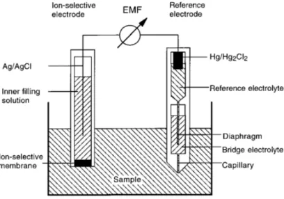
binds with calcium ionophores (L). The +2 charge of the calcium ion causes the deprotonation of two pH indicator molecules, causing the color of the indicators to shift from blue to purple: (Bottom) Molecular structures of the calcium ionophore, charge-balancing additive, and pH indicator. Reproduced with permission from reference 19 (Annual Review of Analytical Chemistry, Vol 7, 2014; Vol. 7, pp 483-512. Copyright 2014, Annual Reviews). ... 5 Figure 1.2 Ion-Selective Electrode Schematic. Reproduced with permission from Reference 21
(Carrier-Based Ion-Selective Electrodes and Bulk Optodes. 1. General
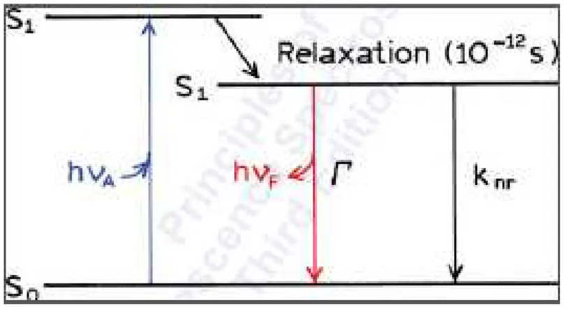
Characteristics. Chemical Reviews 97 (8), 3083-3132. Copyright (1997) American Chemical Society). ... 11 Figure 1.3 Jablonski Diagram. Absorption of a photon excites an electron to an excited singlet
state. Relaxation to a lower energy excited state is known as internal conversion and conversion to an excited triplet state is known as intersystem crossing. The return to the ground state causes the release of a new photon. Reproduced with permission from reference 79 (Principles of Fluorescence Spectroscopy: Third Edition.
Copyright (2006) Springer Science and Business Media, LLC). ... 15 Figure 1.4 Simplified Jablonski diagram showing quantum yield and fluorescence lifetime.
Reproduced with permission from reference 79 (Principles of Fluorescence Spectroscopy: Third Edition. Copyright (2006) Springer Science and Business
Media, LLC). ... 16 Figure 1.5 Three equilibrium expressions to determine ionophore-based sensor response: (1)
Extraction of the target ion into the sensor phase, corresponding with a release of hydrogen, (2) target ion binding with the ionophore, and (3) acid/base equilibria of the pH indicator. Reproduced with permission from reference 19 (Annual Review of
Analytical Chemistry, Vol 7, 2014; Vol. 7, pp 483-512. Copyright 2014, Annual
Reviews). ... 18 Figure 1.6 Theoretical O2 concentration profile at surface of an enzyme-linked nanosensor. (A)
The lower limit of the sensors dynamic range corresponds to an analyte concentration that cause an O2 gradient to form at the sensor surface at the
nanosensor surface based on the enzyme-catalyzed reaction. (B) The upper limit of the sensor’s dynamic range corresponds to an analyte concentration that depletes all O2 at the nanosensor surface based on the enzyme-catalyzed reaction. ... 22
Figure 2.7 Sensor mechanism. Nanosensors loaded with an oxygen-responsive fluorescent dye have the enzyme glucose oxidase (GOx) conjugated to their lipid layer. When the local glucose concentration increases, a reaction between glucose and oxygen and glucose is catalyzed by GOx, reducing the local oxygen levels and increasing the fluorescence of the oxygen-responsive dye. Nanosensors also contained iron oxide (Fe3O4) nanoparticles for magnetic control. ... 32
x
Figure 2.8 Biotin/Avidin based conjugation strategies. (Left) NSB-A-BGOx particles consist of typical nanosensor formulations created with a substituted biotinylated lipid and mixed in solution with free avidin linker (A) and biotinylated glucose oxidase (BGOx). (Right) NSB-AGOx particles consist of typical nanosensor formulations created with a substituted biotinylated lipid and mixed in solution with avidinylated glucose oxidase (AGOx). ... 33 Figure 2.9 Effect of enzyme concentration (BGOx) on NSB-A-BGOx sensor response. Kinetic
traces of sensor response with high (A), medium (B), and low (C) concentrations of BGOx. Analysis of initial slope across the test range of glucose concentrations shows fastest response to high BGOx, slower response to medium, BGOx, and a
minimal response to low BGOx (D)... 37 Figure 2.10 Combined, normalized dose/response curves for nine batches of NSB-A-BGOx
sensors over seven unique avidin levels, generated by plotting the initial slope of the kinetic trace against glucose concentration for each sensor batch (A). Response midpoint (LogEC50) vs. avidin amount, showing a minimum LogEC50 (maximum
responsiveness) in the range of 0.11-0.44 mg avidin (B). ... 38 Figure 2.11 Effect of surface biotinylation on response of NSB-A-BGOx particles. Higher
surface biotinylation (A) leads to a stronger response to glucose than a lower amount of surface biotinylation (B). ... 39 Figure 2.12 Response tuning with NSB-AGOx sensors based on surface biotinylation. Kinetic
traces of sensor response to a range or glucose for 100% (A), 25% (B), 1% (C), and 0% (D) biotinylation... 40 Figure 3.1 Graphical Abstract. The dynamic range of ionophore-based nanosensors is
controllable through changes to the indicator composition. ... 49 Figure 3.2 Mechanism of IBOS response to increasing analyte (I+) concentration with two pH
indicators (Ind1 and Ind2) co-loaded into a sensor matrix with additive (R-), and ionophore (L). At low analyte concentration, both pH indicators are protonated and both give off a fluorescent signal. At a higher concentration, the analyte begins to diffuse into the sensor and binds to the ionophore that in turn deprotonates the pH indicator with the lower pKa. At high analyte concentrations, both pH indicators
begin to deprotonate until a point where there is no signal from either molecule at the selected wavelength. ... 52 Figure 3.3 Theoretical normalized protonation dose-response curves for lithium-sensitive
IBOS. (A) Mixed nanosensor method: changing does not impact how the pH indicators deprotonate. (B) Mixed optode method: By mixing the pH indicators together in one sensor, the thermodynamics of deprotonation change based on . The linear range and EC50 shifts toward higher concentrations as Ind2 is replaced
with Ind1. ... 55 Figure 3.4 Theoretical normalized dose-response curves. Solid red curves represent the mixed
optode method while dashed black curves represent the mixed nanosensor method. increases from 0 to 1 at an increment of 0.2 from right to left. While the
xi
deprotonation of the individual pH indicators is very different, the detectable
combined-fluorescent output is similar between the two methods at any value of . .... 56 Figure 3.5 Mixed optode lithium-sensitive IBOS response. (A) Normalized fluorescence
dose-response curves. increases from 0 to 1 as the color shifts from blue to pink. (B) The linear range and LogEC50 shifts toward lower concentrations as ChII is replaced
with ChVII. ... 61 Figure 3.6 Control of LogEC50 with sensor composition. More deviation from theory observed
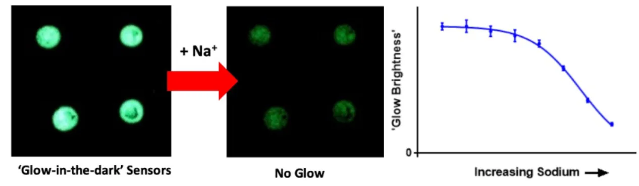
with the mixed optode method than with the mixed nanosensor method. ... 62 Figure 4.1 Graphical Abstract. The brightness of the ‘glow’ emanating from the sensor
decreases as the sodium concentration increases ... 69 Figure 4.2 Glow Sensor mechanism. A charge balancing additive holds the Blueberry
dye in a protonated state in the absence of sodium. Sodium from the test sample is extracted into the sensor core where it binds with the ionophore. Charged sodium ions force the deprotonation of the Blueberry dye to maintain electroneutrality in the organic phase. When deprotonated, the Blueberry dye absorbs photon emission from the persistent luminescence microparticles at a higher rate, minimizing the observed phosphorescence. ... 72 Figure 4.3 Signal analysis for Glow Sensor spots. The Blueberry dye in the sensor turns
from clear to blue upon deprotonation, increasing the absorbance of the glow from the persistence luminescence microparticles, thereby decreasing the amount of measured luminescence in basic solution. Due to the presence of sodium ionophore, the addition of sodium causes the same deprotonation of the Blueberry dye. (A) Phosphorescent decay curves (n=3) from a single sensor spot averaged together at increasing sodium concentrations. Dotted lines show area of integration used to calculate sensor response. (B) Dose/response curve showing average response to sodium of the four
individual sensor spots. This shows that the sensor phosphorescence decreases as a function of sodium concentration. (B, inset) images of the phosphorescent spots under acidic (bright) and basic (dim) conditions. ... 74 Figure 4.4 Full glow sensor characterization. (A) Sensor signal after addition of 100 mM
sodium. Response time of the sensor is 9.6 minutes (T95). (B) Reversibility of the
sensor analyzed by exposing sensor to alternating solutions of 0 mM and 100 mM sodium. (C) The sensor is highly selective against the potentially interfering ions Li+
and K+. (D) The sensor response to sodium is stable over 14 days. ... 76
Figure 5.1 EnzNS under ‘steady-state’ operation. Sensors are sealed in a microdialysis tube, adhered to the bottom of a well plate, and HEPES/TRIS solution is added on top. (A) A 3x7 area scan is taken of the center of the well every minute for 6 minutes before the glucose solution is changed and the scan is repeated. (B) The 7 points of interest from the brightest (middle) row of the area scan are processed into a
dose/response curve... 84 Figure 5.2 Dual-ionophore use for dynamic range tuning with (A) mixed optode method and
xii
dynamic range can be adjusted without dual-ionophore use, but at the loss of signal-strength ... 85 Figure 5.3 (A) The silicon nanocrystal sensor is selective for sodium against potentially
interfering cations (B) and is responsive for at least one week. ... 86 Figure A.1 Demonstration of enzyme/nanosensor separation scheme. ELiNS and EnzNS
undergo three rounds of magnetic separation and purification to remove unbound GOx from the magnetic nanosensors. EnzNS formulations (without avidin) have no attachment between the magnetic nanosensors and enzyme, so all enzyme is removed and the nanosensors lose their responsiveness to glucose. ELiNS formulations (with avidin) contain linkages between enzyme and the magnetic
nanosensors, and so they retain their responsiveness to glucose after separation. ... 90 Figure A.2 Triplicate data for NSB-A-BGOx sensors with highest enzyme loading (1 mg). ... 90 Figure A.3 Kinetic traces for three separate experiments that explored the effect of seven avidin
levels on NSB-A-BGOx sensor response. The first experiment explored low levels of avidin (A, B, and C), the second explored intermediate levels of avidin (D, E, and F), and the third explored high levels of avidin (G, H, and I). Low enzyme activity is observed with low amounts of avidin (0.02 and 0.05 mg), and slightly diminished enzyme activity is observed with high avidin amounts (0.88 and 1.32 mg). ... 91 Figure A.4 Response to 4mM in the low avidin experiment (A), the intermediate avidin
experiment (B), and the high avidin experiment (C). Summary of response to 4 mM glucose across the three experiments, with error bars showing standard deviation between overlapping levels of avidin (0.11 mg and 0.44 mg) tested between the two experiments (D). ... 92 Figure A.5 Effect of surface biotinylation on response of NSB-A-BGOx particles. Replica of
Figure 4 with a narrow y-axis range in panel B showing that the sensors are still
slightly responsive to glucose at 6.3% biotinylation. ... 92 Figure A.6 Dose response curve generated by plotting initial slope of kinetic trace vs. glucose
concentration for NSB-A-BGOx particles with different amounts of surface
biotinylation. ... 93 Figure A.7 Dose/response curves for NSB-AGOx sensors. ... 93 Figure A.8 TEM image of Fe3O4 nanoparticles in nanosensors. The darker shaded circles show
nanosensors with no Fe3O4 nanoparticles encapsulated (blue, top), a low amount of
Fe3O4 nanoparticles encapsulated (red, lower left), and a high amount ofFe3O4
nanoparticles encapsulated (green, lower right). ... 94 Figure B.1 Theoretical predictions of mixed optode (red solid lines) and mixed nanosensor
(black dashed lines) dose-response curves when both pH indicators have the same maximum fluorescence. ... 97 Figure B.2 Nanosensor response curves using theoretical predictions from the mixed optode
theory at various pH indicator pKa separations. Blue curves show the response of
xiii
indicator 2 and solid purple lines are the response of the mixed optode approach
with = 0.5. ... 98
Figure B.3 Nanosensor response curves using theoretical predictions at various pH indicator pKa separations. Blue curves show the response of sensors made with indicator 1, pink curves show the response of sensors made with indicator 2 and solid purple lines are the response of the mixed nanosensor approach with = 0.5. ... 99
Figure B.4 Absorbance spectra of lithium-selective IBOS with (A) ChII or (B) ChVII... 100
Figure B.5 Emission Spectra of lithium-selective IBOS with (A) ChII or (B) ChVII after 660 nm excitation. ... 100
Figure B.6 Mixed nanosensor lithium-sensitive IBOS response. (A) Normalized fluorescence dose-response curves. increases from 0 to 1 as the color shifts from blue to pink. (B) The linear range and LogEC50 shifts toward lower concentrations as ChII is replaced with ChVII. A * represents a significant difference in LogEC50 with p < 0.05; **p < 0.01; ***p < 0.001; ****p < 0.0001. ... 100
Figure B.7 Dynamic range extension of lithium-selective IBOS. ... 101
Figure B.8 Apparent overall equilibrium constant vs. . ... 101
Figure B.9 Single-Chromoionophore control experiment. Changing the concentration of chromoionophore VII changes only the intensity of the nanosensor without affecting the LogEC50. ... 101
Figure B.10 Response of single-pH indicator nanosensors and dual pH indicator nanosensors made with the mixed optode method to lithium, sodium, and potassium. ... 102
Figure B.11 Control of nanosensor response with mixed optode method in PBS solution... 102
Figure B.12 (A) Dose/response curve obtained from sample with unknown lithium content. Two capsules of lithium orotate were dissolved in 40 mL HEPES/TRIS and then diluted by a factor of ten, five times. (B) Dose/response curve obtained from dilutions of lithium at known concentration. The x-axis value of ‘test sample’ (-1) was shifted by the difference in LogEC50s between the two curves, and then the lithium content of one pill was back-calculated. ... 102
Figure B.13 Mixed optode method for calcium-sensitive IBOS. ... 103
Figure B.14 Mixed nanosensor method for calcium-sensitive IBOS. ... 103
Figure B.15 LogEC50 tuning of calcium-sensitive nanosensors. ... 103
Figure B.16 Dynamic range extension of calcium-sensitive nanosensors. ... 104 Figure C.1 (Left Column) Glow Sensor luminescence (fluorescence and phosphorescence when
the shutter is open, phosphorescence only when the shutter is closed) during shutter program for four spots: A, B, C, and D. (Right Column) The average of the three
xiv
phosphorescent decay curves collected while the shutter is closed for spots A, B, C, and D ... 109 Figure C.2 Spot A under basic conditions compared to background (no sensor) signal. This
shows that the phosphorescence is predominantly quenched by full deprotonation of the blueberry dye, although some residual signal remains. ... 110 Figure C.3 Luminescent signal from the Glow Sensor compared to background noise over time
after ending excitation. The trend is described by a two-phase exponential decay
with a fast half-life of 1.6 seconds and a slow half-life of 14.08 seconds. ... 110 Figure C.4 (Left column) Luminescence during shutter program for Glow Sensor spots without
Blueberry dye. (Right Column) Averaged phosphorescent decay curves for Glow Sensor spots without Blueberry dye. ... 111 Figure C.5 (Left) Dose/Response curve for Glow Sensor spots made without Blueberry Dye.
Minimal response to Na+ is observed. (Right) Glow Sensor spots made without
persistent luminescence microparticles show no phosphorescence under acid and base conditions (see Fig S2 red curve for comparison of background signal). Time zero in this panel is the time when the shutter is closed and the excitation source
blocked from the sample. ... 112 Figure C.6 (Top) Absorbance of an optode spot made without phosphorescence microparticles
under acidic and basic conditions, showing a change in absorption over a wide range. (Bottom) Phosphorescent spectra of Glow Sensor (Blue) and no-blueberry dye control spot made without blueberry dye (Red) under acidic (solid circles) and basic (hollow circles) conditions. This demonstrates that the glow sensor
phosphorescence is greatly reduced in basic conditions, which corresponds with a rise in absorbance from the blueberry dye at the same range of wavelengths. Without blueberry dye, however, the Glow Sensor does not change its phosphorescence between acidic and basic conditions. The energy coupling between the blueberry dye and phosphorescent microparticles is likely either due to the inner filter effect or from resonance energy transfer, both of which would require a rise in absorbance in the blueberry dye to correspond to a decrease in phosphorescence from the
phosphorescent microparticles. ... 113 Figure C.7 Luminescence during extended shutter program for Glow Sensor spots during
response time experiment. ... 114 Figure C.8 Drift of Glow Sensor α50 over the course of the experiment. ** represents a
significant difference in α50 with p < 0.01. ... 114
Figure C.9 (Left) Dose/Response curve and (Right) dynamic range for spots A, B, C, and D. ... 114 Figure C.10 Compilation of all Glow Sensor dose/response curves demonstrating excellent
xv
LIST OF TABLES Table 1.1 Commercially Available Sodium Ionophores Table 1.2 Commercially Available Potassium Ionophores Table 1.3 Commercially available Lithium Ionophores Table 1.4 Commercially Available Calcium Ionophores Table 1.5 Commercially Available Magnesium Ionophores Table 1.6 Commercially Available Chromoionophores
xvi
LIST OF TERMS, SYMBOLS, AND ABBREVIATIONS LiNS: Lihtium detecting nanosensor
Ch: Chromoionophore NaI: Sodium Ionophore CaI: Calcium Ionophore LiI: Lithium Ionophore Ind1: Indicator 1 Ind2: Indicator 2
ISE: Ion selective electrode Fe3O4NP: Iron oxide nanoparticle
ChII: Chromoionophore II ChVII: Chromoionophore VII Ind1: Indicator 1
Ind2: Indicator 2
ULR: upper linear range LLR: lower linear range L: analyte-binding ligand R-: charge-balancing additive I+: cation
Enzyme-coupled nanosensor (EnzNS): a general term for any nanosensor that uses an enzyme as its recognition element
Enzyme-associated nanosensor: an enzyme/nanosensor platform where the two are simply mixed together with no attempt for chemical binding
Enzyme-linked nanosensor (ELiNS): an enzyme/nanosensor platform where the two are bound to each other with some type of chemical bond
Mixed Optode Method: A method of creating a dual-chromoionophore or dual-ionophore nanosensor platform where both chromoionophores or both ionophore are loaded into a single nanosensor
xvii
Mixed Nanosensor Method: A method of creating a dual-chromoionophore or dual-ionophore nanosensor platform where two batches of single-chromoionophore or single-ionophore sensors are created and then mixed together in different ratios
EnzNS: Enzyme-coupled nanosensors (a solution of enzymes and polymeric nanosensors with no specific interaction between the two entities)
ELiNS: Enzyme-linked nanosensors (a structure that consists of enzymes conjugated to a polymeric nanosensor with a specific interaction holding them together)
GOx: Glucose oxidase
AGOx: Avidin/glucose oxidase conjugates BGOx: Biotin/glucose oxidase conjugates
NSB-A-BGOx sensors: ELiNS consisting of polymeric nanosensors with biotin groups on the surface and an avidin linker connecting BGOx to the nanosensors
NSB-AGOx sensors: EliNS consisting of polymeric nanosensors with biotin groups on the surface to which AGOx is bound
xviii
ACKNOWLEDGEMENTS
First, I would like to thank my advisor, Professor Kevin J. Cash, for inviting me to his research group and for supporting me through the entire process. Specifically, I want to thank him for his constant enthusiasm for science and for teaching me, and trusting me, to think independently from day one. Additionally, I want to thank the rest of my committee, Professors Kim Williams, Ning Wu, and Keith Neeves for their valuable advice and continued guidance for my research plans, and for teaching me in depth on the subjects of analytical chemistry, soft matter, and bioengineering. I consider the knowledge I gained in each of these subjects to be essential to my Ph.D. education.
I want to thank Dr. Anne Galyean for her guidance through the Ph.D. process, her career advice, and for helping me learn to mountain bike without crashing, an essential component of any Colorado-based Ph.D. program. I also want to thank my officemates, Dr. Anne Galyean, Aakash Katageri, and Megan Jewell for help working through experimental problems, for the lively discussions, and for making the office and lab an enjoyable place to work. Additionally, I want to thank all of my labmates for their hard work and support, especially Greta Gohring, Makayla Elms, and Madeline Behr for their help with data collection in my publications.
In addition to the knowledge gained about chemical engineering, analytical chemistry, polymeric nanosensors, and the scientific process, I found the Ph.D. process to be incredibly valuable in expanding my worldview and building personal relationships over shared suffering and the pursuit of common goals. For that I want to thank all of my classmates in the CSM Chemical and Biological Engineering program and all of my CSM triathlon teammates. Finally, I want to thank all of my housemates, including Kate Sciamanna, Javier Vargas-Johnson, Scott Nicholson, Tommy Feurst, John Czerski, Alexis Dubois, Meriel Young, Dr. Tadesse Weldu, and Andrew Schied for ensuring there were never any dull moments in my life and for making Golden an affordable place to live.
Most importantly, I would like to thank my parents for the 28 years of encouragement, motivation, patience, and moral support necessary to complete a Ph.D.
1 CHAPTER 1
GENERAL INTRODUCTION
1.1 General Introduction
Bioanalysis
Key research, engineering, and healthcare decisions are based on analyte concentration data collected during human health and biological monitoring. The standard approach in modern health care is a medical professional collecting a sample (e.g. blood, urine, saliva) for offline analysis. This procedure is effective for providing a snapshot of analyte levels in a patient, but it comes with significant limitations. Fluctuations in analyte levels cannot be detected without repeated sample collection, an inconvenience for both the patient and provider. Furthermore, analysis is restricted to being performed at health institutes where the proper equipment is available. In addition to clinical use, analyte monitoring is important in cell cultures and 3D cellular meshworks which are often used for drug development.1 Improved analyte monitoring technology can help quantify the chance a new compound has for clinical success. The potential for improvement in new drug development, where the recent trend has been an increase in research and development spending and a decline in clinical success rate,2 is profound. Analyte monitoring also provides insight into questions of scientific interest such as the basis of neuronal signaling in bacterial cultures.3 These examples represent just a small number of the numerous scientific and medical fields where analyte monitoring plays a key role. The continued development of new methods to improve data collection will lead to more accurate diagnoses, better treatment plans, faster technology development, a more efficient allocation of resources, and scientific insight. Bioanalytical Sensors
A device used to quantify analyte concentration is known as a sensor. A distinction should be made between sensing and detection in that detection requires merely determining whether an analyte is present or not (above a certain threshold), whereas sensing requires quantifying the amount of analyte present. Any sensor used for biological analysis is known as a bioanalytical sensor, whereas the term biosensor is reserved for sensors that contain a biological element (e.g. DNA fragments, enzymes).4 The field of bioanalytical sensing is complex and a wide variety of
2
sensors with overlapping classifications have been developed for various applications. However, all sensors must consist of an analyte recognition element and a signal transduction element.4-6 For a limited number of analytes, a single element can serve both purposes,7, 8 but usually two separate elements are used and must be couple together. Classification of bioanalytical sensors is usually based on the sensing mechanism, the signal transduction mechanism, or by the physical shape, structure, and material make-up of the device. Due to the diversity of applications, no one sensor attribute dominates the entire field, but for many in vivo sensing applications, a list of desirable traits includes biocompatibility, miniature size, reversibility/reuse, low invasiveness, the ability for spatial mapping, and ability for continuous detection.9
Polymeric Nanosensors
Luminescent polymeric nanosensors are a relatively new sensor technology with significant advantages over more established sensor types that give them the potential to answer challenging biological questions through advancements in the field of bioanalytical monitoring. Polymeric nanosensors are a miniaturized form of bulk optode membrane sensors, made by dissolving the optode components (e.g. polymer, plasticizer, recognition groups) in organic solvent and emulsifying that solution with an amphiphilic lipid surfactant. This results in water-soluble spherical nanoparticles ~180 nm in diameter. The nanosensor size makes them minimally invasive and biocompatible for in vivo and in vitro use and gives them the ability to create spatial maps of analyte concentrations. Being an emerging sensor technology, more research and development is needed to unlock the potential of nanosensors to solve challenging, real-world problems where other sensor classes fall short.
1.2 Literature Review
1.2.1 Analytes of Interest
In this thesis, we present sensor designs for detecting three different analytes (glucose, lithium, and sodium) with a focus on bioanalytical applications (i.e. cell culture analysis and in vivo physiological monitoring). Therefore, we formulated the sensors for higher analyte levels near physiological concentrations and do not intend for them to be applied for trace detection. Glucose, lithium, and sodium have extensive analytical interest in numerous fields.
3
Sodium is a monovalent cation that is essential to maintaining normal physiological function. Hyponatremia, a condition of low blood sodium concentration, is the most common electrolyte disorder.10 Dysfunction of sodium channels in the brain has been implicated in epilepsy, long QT syndrome, heart failure, and other diseases.11 Continuous sodium sensors have been developed for monitoring plasma blood electrolyte levels12 and creating spatial maps of sodium activity during action potentials in isolated cardiomyocytes.11
Lithium is a monovalent cation that is considered one of the five biologically most important alkali and alkaline earth metal cations.13 Ionic lithium acts as a mood stabilizer14 and is most commonly used for the treatment of manic-depressive disorder. After intake as a therapeutic drug, the actual concentration of lithium in the blood varies from person to person and therefore must be monitored regularly to ensure proper dosage.13
Glucose plays an essential role in many cellular processes, including cellular respiration. The most prevalent example of glucose monitoring is for diabetes, a well-known chronic, metabolic disorder that results in abnormal glucose levels. Diabetes is a major cause of blindness, kidney failure, heart attacks, stroke, and lower limb amputation and in 2012 an estimated 1.5 million deaths were caused by diabetes while another 2.2 million deaths were caused by high blood glucose.15 Because of the inherent dangers, it is critical for diabetics to closely monitor their blood glucose. The World Health Organization estimates there to be 422 million people in the world and 8.5% of people over 18 years of age to have diabetes as of 2014.15 Because of this large demand, roughly 85% of the current biosensor market is for glucose sensors.16 While in this work we focused on these three analytes, the methods we developed are applicable to many small cations, anions, and molecular targets through simple, well-known formulation changes.
1.2.2 Overview of Bioanalytical Sensors
Sensor design is often thought of in terms of analyte recognition and signal transduction: Some aspect of the sensor must be able to determine the presence of the intended analyte and that recognition event must trigger a change in some property of the sensor that can be measured with available equipment.5 Greater quantities of the analyte should trigger larger measurable changes
for the device to be considered a sensor instead of a detector. For a select group of analytes, one element can serve as both recognition element and signal transducer, a strategy referred to here as
4
direct detection. This is exemplified by pH indicator dyes – where the protonation/deprotonation event directly changes the dye color.7 However, to reach a greater number of analytes, separate elements are used for analyte recognition and signal transduction and must be coupled together, a strategy known here as indirect detection. An example is the modern immunoassay, where an antibody recognizes a target protein, and then a secondary signal is generated by other sensor components.17, 18 Modern polymeric nanosensors usually rely on one of two indirect strategies for analyte recognition (ionophore-based and enzymatic) and mostly use light emission for signal transduction. Ionophore-based recognition19, 20 is used to build ion sensors, while enzymatic approaches9 are used to reach small biomolecule targets. Both strategies were initially developed
for electrochemical sensors5 and later used in bulk optode sensors,20, 21 which are earlier generation
sensor classes that led to the development of polymeric nanosensors.
1.2.2.1 Detection Strategies
Organic Fluorescent Molecular Dyes
Organic fluorescent molecular dyes are a class of natural and synthetic molecules with fluorescent properties. While fluorescent dyes are commonly used for imaging purposes where their only duty is to render cells or specific structures fluorescent and therefore visible through microscopy, some dyes have intrinsic sensing capabilities, meaning they are able to serve both as analyte recognition element and signal transducer (e.g. serve by themselves as a direct sensor).22 However, only a limited number of analyte targets are accessible through fluorescent dyes. A large number of molecules exist that can directly detect oxygen8 and pH,23 while a relatively fewer options exist for ion targets, though recent synthesis efforts are aimed at expanding the available selection.6, 24 These dyes have been deployed for imaging/sensing applications such as biofilm pH analysis25 and have been used to gain insight into key questions of scientific interest such as understanding sodium and potassium dynamics in bacterial ion channels.3 However, use of these dyes without a larger sensor construct for applications such as cellular imaging makes them susceptible to issues such as unwanted binding to proteins, cellular toxicity, and intracellular sequestration.26 Use of free fluorescent dyes also limits their capacity for optimized response and
5 Ionophore Recognition
Ionophore-based strategies21 are based on molecules which can reversibly bind to specific ions, known as ionophores. Ionophore use began in 1964 after a discovery by Moore and Pressman that some antibiotics induce ion transport in mitochondria.27 Simon and Stefanac soon investigated further and found that the phenomenon is due to the selective formation of these complexes and certain cations.28 Around the same time, some groups were synthesizing macrocyclic polyethers and macroheterobicyclic compounds and showed their utility for complexing alkali and alkaline-earth metals.29 In a few years, many natural and synthetic ionophores were realized21 and soon
they were being used in ion-selective electrodes, a type of electrochemical sensor, for cation sensing.30
Figure 1.1 (Top) Schematic of sensing mechanism for an ionophore-based bulk optode sensor made with a calcium ionophore with a 3:1 complex ratio. A charge-balancing additive is used to hold the pH indicators (Ind) in a protonated state in the absence of Ca2+. As Ca2+ increases in the
sample, it is extracted into the sensor film where it binds with calcium ionophores (L). The +2 charge of the calcium ion causes the deprotonation of two pH indicator molecules, causing the color of the indicators to shift from blue to purple: (Bottom) Molecular structures of the calcium ionophore, charge-balancing additive, and pH indicator. Reproduced with permission from reference 19 (Annual Review of Analytical Chemistry, Vol 7, 2014; Vol. 7, pp 483-512. Copyright 2014, Annual Reviews).
6
Since ionophores are typically optically silent, they are paired with a fluorescent pH indicator and a charge balancing additive for use in optical sensors such as bulk optodes and polymeric nanosensors. The fluorescent pH indicator is usually from a family of organic fluorescent indicators derived from the molecules Nile blue and fluorescein known as chromoionophores that exist in an acid/base equilibrium and change color as they shift their protonation state. The response of ionophore-based sensors is then based on a model of thermodynamic equilibrium (see Section 1.2.3.2) that takes into account the binding strength of the ionophore and the protonation state of the chromoionophore, coupled together by charge balance in the sensing phase. The mechanism can be thought of in three steps, illustrated in Figure 1.1: (1) analyte extraction from the sample into the sensing phase, (2) analyte binding with the ionophore, and (3) deprotonation of the pH indicator, causing a change in fluorescence. Realistically, these three steps are all equilibrium reactions happening simultaneously, but do highlight the three distinct equilibria.
Important considerations when choosing an ionophore during sensor design are the complexing coefficient and the equilibrium constant (β). The equilibrium constant is known to change depending on the dielectric constant of the local environment.31 Likewise, the pKa of the
chromoionophore should be considered, as well as the charge of the chromoionophore, and it should be taken into account that the local dielectric constant can affect the observed pKa.7, 32-34 Present day, there are a wealth of ionophores available commercially for common cations such as Na+ (Table 1.1), K+ (Table 1.2), Li+ (Table 1.3), Ca+ (Table 1.4), and Mg2+ (Table 1.5). A list of commercially available chromoionophores is shown in Table 1.6. Tables 1.1-1.6 also show equilibrium constants and complexing coefficients in different environments for select compounds.
Table 1.7 Commercially Available Sodium Ionophores
Sodium Ionophore35 Alternate name Log(β) in BEHS31 Log(β) in NPOE31 Complexing Coefficient (n)31 I ETH 227 II ETH 157 7.71±0.05 9.41±0.11 2 III ETH 2120 8.76±0.05 10.91±0.04 2
7
Table 1.1 Commercially Available Sodium Ionophores (continued)
IV DD-16-C-5 V ETH 4120 VI 6.55±0.06 9.19±0.11 1 VIII X 7.69±0.05 10.27±0.05 1
Table 1.8 Commercially Available Potassium Ionophores
Potassium Ionophore35 Alternate name Log(β) in DOS31 Log(β) in NPOE31 Complexing Coefficient (n)31 I Valinomycin 10.1±0.07 11.63±0.08 1 (assumed) II BB15C5 7.84±0.02 10.04±0.01 1 III BME 44 6.88±0.05 10.22±0.07 1 IV
Table 1.9 Commercially available Lithium Ionophores
Lithium Ionophore35
Alternate
name Log(Beta) in NPOE31
Complexing Coefficient (n) 31 I ETH 149 10.71±0.04 2 II ETH 1644 8.24±0.04 2 III ETH 1810 8.77±0.02 2 IV V VI 5.33±0.03 1 VII VIII 10.40±0.07 1
Table 1.10 Commercially Available Calcium Ionophores
Calcium
Ionophore35 Alternate name
Log(β) in DOS31 Log(β) in NPOE31 Complexing Coefficient (n) 31 I ETH 1001 19.70±0.07 24.54±0.09 2 II ETH 129 25.5±0.1 29.2±0.2 3
8
Table 1.4 Commercially Available Calcium Ionophores (Continued)
III
Calimycin, Antibiotic A
23187 8.67±0.07 12.93±0.18 2
IV ETH 5234 22.06±0.08 27.39±0.04 3
VI
Table 1.11 Commercially Available Magnesium Ionophores
Magnesium Ionophore35 Alternate name Log(β) in DOS31 Log(β) in NPOE31 Complexing Coefficient (n) 31 I ETH 1117 9.72±0.18 13.84±0.16 3 II III ETH 4030 7.25±0.11 12.15±0.11 2
Table 1.12 Commercially Available Chromoionophores
Chromo-ionophore35 Alternative Name pKa32 pKa in PVC/DOS33 pKa in PVC/NPOE 33 pKa in membrane (PVC/ DOS)7 Derivative Family
I ETH 5294 11.1±0.1 11.41±0.03 14.82±0.03 12 Nile Blue
II ETH 2439 9.16 ± 0.02 12.3± 0.02 10.2 Nile Blue III ETH 5350 8 ± 0.04 9.59± 0.04 13.4 Nile Blue IV ETH 2412 17 ± 0.04 20.49±0.03 V Nile Blue VI ETH 7075 12.53 ± 0.01 15.43±0.05 Fluoroscein
VII ETH 5418 8.56 ± 0.004 11.72±0.06 9 Nile Blue
VIII TBPE IX ETH 4003 XI ETH 7061 18.04 ± 0.01 20±0.04 Fluoroscein XV ETH 4001 XVII GJM-541
9 Enzymatic Recognition
Enzymatic recognition was used by Clark and Lyons in 1962, in the first biosensor described in the literature.36 They coupled the enzyme glucose oxidase, which catalyzes the oxidation of glucose according to Equation 1.1, to an amperometric electrode that could measure 𝑃O2.
𝛽 − 𝐷 − 𝐺𝑙𝑢𝑐𝑜𝑠𝑒 + 𝑂2 → 𝐷 − 𝑔𝑙𝑢𝑐𝑜𝑛𝑜 − 1,5 − 𝑙𝑎𝑐𝑡𝑜𝑛𝑒 + 𝐻2𝑂2 (1.1)
The concentration of glucose in the sample was shown to be proportional to the lowering of 𝑃O2 which was sensed by the electrode. In the following several years, this type of sensing mechanism was adopted to make sensors for other small biomolecule targets by combining an existing electrode with the appropriate enzyme.37 The wide variety of oxidase enzymes available (e.g. enzymes that catalyze the oxidation of some small biomolecule with the depletion of O2) makes it
easy to change the sensor target with by replacing the oxidase enzyme and retaining O2 based
signal transduction method. Equation 1.1 also causes a local drop in pH, meaning that pH reporters can be utilized for signal transduction. Goldfinch and Lowe demonstrated this concept in 1984 for penicillin, urea, and glucose using the appropriate enzymes.38 Enzymatic recognition can also be used with optical bulk optode membrane sensors,39, 40 though ionophore-based mechanisms are far more common with this sensor class. While polymeric nanosensors are also more commonly designed with ionophore-based mechanisms, they have been shown to be compatible with enzyme-based mechanisms41, 42 and their viability for us in in vivo mice studies has been demonstrated.41
Other recognition strategies
While ionophores are key for ion detection and enzymes are key for small bio-molecule detection, other strategies are need to branch outside of these two families of analytes.20 Antibodies
are naturally occurring protein structures that are deployed by the immune system for recognition and elimination of harmful foreign substances. As a result, their excellent analyte target specificity and affinity can be utilized in sensor devices for detection of a large number of disease markers, food and environmental contaminants, biological warfare agents, and illicit drugs.43 Nucleic acid sequences can be formulated for the recognition of specific DNA fragments through highly specific base-pair sequence matching.44 Similarly, single-stranded oligonucleotide sequences
10
known as aptamers can be made to have high binding affinities for select analytes through an iterative selection process from large random sequence pools. Aptamers have been isolated to bind to a wide variety of analytes including ions, small molecules, proteins, and whole cells.4, 45 In addition to the above ‘natural’ recognition elements, analyte receptors can also be synthesized such as with molecularly imprinted polymers (MIPs). MIPs are templated polymer matricies that are design to achieve specific binding with a target analyte by creating size- and shape- specific pockets.46 These recognition strategies are potential avenues for expanding the range of analytes
accessible with the polymeric nanosensor platform.
1.2.2.2 Sensor Classifications
Modern day polymeric nanosensors are the result of miniaturization of optical bulk optode membrane sensors, often referred to simply as ‘optodes,’ meaning they consist of the same sensor components and utilize the same response mechanisms but simply differ in packaging. Many of the response mechanisms used with bulk optode sensors originated from the reports on electrochemical sensors that came earlier and adjusted for optical signal transduction. Because of this progression, referring to the literature on bulk optodes and electrochemical sensors is often helpful for the design and development of polymeric nanosensors.
Electrochemical
An electrochemical sensor is generally defined as any sensor with an electrochemical signal transduction element, which can take the form of amperometry, potentiometry, and conductometry among other methods.5 Electrochemical sensor reports predate those of bulk optode membranes or polymeric nanosensors,36 making them more robust and more fully studied. Among the most relevant subclassifications of electrochemical sensors for polymeric nanosensors are selective electrodes and enzyme-based electrochemical films. The essential feature of ion-selective electrodes (ISEs) and many other electrochemical sensors is the solvent polymeric membrane (i.e. plasticized polymeric matrix), which is a water immiscible, high viscosity liquid used to house hydrophobic sensing components. James Ross47 and Adam Shatkay48 introduced the use of plasticized polymer matrices into sensor concepts in 1967 in their respective calcium sensor reports. Since then, poly(vinyl) chloride (PVC) quickly became widely accepted as the standard polymer material,21, 49 often paired with bis(2-ethylhexyl) sebacate as a plasticizer, though other
11
membrane materials are sometimes used as well. For use in ISEs, this sensing membrane is placed between the sample and an internal electrolyte solution and responds to the activity of the target ion, as shown in Figure 1.2.
Figure 1.2 Ion-Selective Electrode Schematic. Reproduced with permission from Reference 21 (Carrier-Based Ion-Selective Electrodes and Bulk Optodes. 1. General Characteristics. Chemical Reviews 97 (8), 3083-3132. Copyright (1997) American Chemical Society).
Electrochemical sensors such as ISEs have extraordinarily large measurement ranges that can span from about 1 to 10-6M and are capable of continuous measurements,21 but they require relatively complex devices for signal transduction. Due to the ionophore-based response mechanism, they have cross-sensitivity to pH, though this can be overcome by co-monitoring pH with a separate electrode. They are also not easily miniaturized and cannot monitor two- and three-dimensional spaces without complex sensor arrays. While they have shown some capacity for in vivo sensing applications,50 they have low biocompatibility and require transdermal implantation which invokes an immune response from the host organism.9
Bulk Optodes Membranes
Bulk optode membranes consists of a hydrophobic, solvent polymeric membrane, with millimeter- to centimeter-scale dimensions, that can interface with an aqueous test sample. They utilize many of the same analyte recognition strategies as electrochemical sensors but instead rely
12
on optical signal transduction. The first sensor that closely resembled modern optical bulk optodes was reported by Charlton et al. in 1982.51 The design consisted of simply a plasticized PVC matrix with the commonly used potassium ionophore (i.e. ion-binding molecule) valinomycin and used an anionic dye, erythrosine B, that was mixed with the test sample for an optical signal transduction. The sensor served as an irreversible, single-use test strip. The field grew more rapidly beginning in 1989, when Morf et al. added a lipophilic pH indicator (i.e. chromoionophore) to the sensing phase and monitored its absorbance to make reversible carbonate,52 ammonium,53 and
calcium54 optodes. The concept quickly to include spread to include cation targets such as phenylethylammonium ions,55 lead,56 potassium,57 sodium,58 and zinc.59 Bulk optodes have also
been designed using enzymatic recognition, as described in Section 1.2.2.1 Detection Strategies. The optical signal transduction strategies utilized by bulk optode membranes have a number of advantages over electrochemical sensors. Optical transduction allows for remote data collection, meaning analyte monitoring can occur without bulky devices that interfere with the samples they are trying to measure. While still being too bulky for ideal in vivo use, bulk optodes are more amenable to miniaturization and alterations to make them more biocompatible, which has been the focus of many research efforts since ~1999.
PEBBLES
An important development for bioanalytical sensors came in 1999, when Clark et. al. miniaturized the bulk optode sensor platform to a nanoscale device which they termed PEBBLEs (Probes Encapsulated By Biologically Localized Embedding).26, 60 PEBBLEs consist of spherical polymer spheres, with indicator dyes trapped within the matrix. The PEBBLE sensor construct combined the size advantage of fluorescent indicator dyes with the advantage of the protective polymer matrix that comes with bulk optode sensors. The miniature size of PEBBLEs made them viable for intracellular monitoring, since their total volume is negligible to that of a cell. PEBBLEs also provided the advantage of greatly improved response time (1 ms) since they greatly increase the surface area to volume ratio and therefore reduce the time for analyte diffusion. PEBBLEs were also shown to be compatible with a diverse set of detection mechanisms adopted from bulk optodes and ISE membranes. By simply incorporating hydrophobic, organic fluorescent indicators along with ratiometric dyes, PEBBLEs could be made to directly sense pH, 26 oxygen, 26 calcium,26
13
components (i.e. ionophore, additive, and pH indicator) could be incorporated to reach more ion targets via an ionophore-based mechanism.62 Enzymes could also be incorporated and paired with oxygen-sensitive fluorophores for glucose detection.63
While PEBBLEs were an important sensor advancement that showcased the ability for bulk optode miniaturization, they had several fatal flaws that limited their practical applications and would soon be improved upon with second-generation miniaturized sensor constructs. In addition to the preparation being time-consuming,49 the size of the particles were not well controlled. The
particle synthesis often resulted in a bimodal distribution, and while the majority of the particles per batch would be as small as 20 nm, a majority of the sensor components would be incorporated into a smaller number of larger 200 nm particles.26 But most importantly, PEBBLEs were shown
to leach as much as 50% of the loaded indicator dye over a 48 hour period, limiting their application to short-term use.60
Polymeric Nanosensors
In 2007, many of the negative attributes of PEBBLE sensors were addressed with a report for polymeric nanosensors by Clark and co-workers.64 Instead of the crosslinked polymer matrices used by PEBBLEs, these sensors took the plasticized PVC matrix preferred by bulk optodes and enclosed microscopic spherical particles with an amphiphilic lipid layer through a simple sonication synthesis. These sensors were shown to be stable for about one week and were applied for in vivo applications such as visualizing sodium dynamics in cardiomyocytes11 and in mice.12 The polymeric nanosensor platform has been continually researched since this report and progress is still being made today. In addition to adopting response mechanisms from bulk optode and electrochemical sensors for use in polymeric nanosensors, many new polymeric nanosensor reports showcase new modifications to the ionophore-based and enzyme-based response mechanisms. For example, in order to widen the possible reporters to use with an ionophore-based mechanism, so-called ‘static’ reporters (i.e. luminescence elements that are not sensitive to pH or any other analyte) have been paired with pH-sensitive dyes that can changed the perceived luminescence of the static reporter through a number of mechanisms.20, 65, 66 Bakker and co-workers also pioneered a method for overcoming the pH dependency of ionophore-based mechanisms by operating polymeric nanosensors in an ‘exhaustive sensing mode’ where the sample analyte is completely consumed by the probe.67, 68
14 Other Types of Miniaturized Optical Sensors
In addition to polymeric nanosensors from Clark and co-workers and PEBBLEs, there are variety of other miniaturized optical sensor platforms based on bulk-optode sensors.49 Bakker and co-workers created monodisperse, optode-based beads on the order of several micrometers in diameter with a sonicating particle caster for a many different ion targets including Na+,69 K+,70 Ag+,71 Cl-,72, 73 and NO2-73 among others. Tohda and Gratzl created color-changing optode-based
micron-scale sensor beads through a spray-drying method.74 Adopting both enzymatic and
ionophore-based recognition strategies, they incorporated an array of beads into their “silver sensor,” a bar-shaped device, roughly 250 μm x 2 mm that could simultaneously potassium, sodium, and glucose.75 Finally, they optimized the components with a goal of monitoring
interstitial fluids with the silver sensor implanted under the skin.76 Ruckh et al. demonstrated a polymer-free optode-based nanosensor in an effort to further reduce the sensor size for intracellular experiments.77 Balconis and Clark78 created lipase-degradable optode-based nanosensors with a
solvent displacement method by replacing the PVC/BEHS core with polycaprolactone and a citric acid ester plasticizer. These efforts represent just a few of the many miniaturized platforms based on bulk optode membranes. The relative advantages and disadvantages of each means that no one sensor construct dominates research interest.
1.2.3 Theory
This section covers theoretical aspects of luminescence theory, ionophore-based sensor response, and enzyme-based sensor response that are relevant to the completed work.
1.2.3.1 Luminescence Theory
Luminescence is the process by which a substance emits light. An electron in a luminescent molecule will jump to an excited state (higher energy orbital) upon the input of energy, such as by absorbing a photon. Relaxation of the electron to the ground state from an electronically excited state will then emit a new photon, producing light. Emission from an excited singlet state is known as fluorescence while emission from excited triplet states is known as phosphorescence. The transition from an excited singlet state to the ground state is spin allowed and rapid since the excited electron has the opposite spin of its corresponding electron in the ground state orbital. Phosphorescence is a slower process since a transition from an excited triplet state to the ground
15
state is spin forbidden. To reach an excited triplet state, the electron must additionally undergo a change in spin, known as intersystem crossing. Photon emission rates for fluorescence are on the order of 108 s-1 while photon emission rates for phosphorescence are on the order of 103 to 100 s
-1.79
Figure 1.3 Jablonski Diagram. Absorption of a photon excites an electron to an excited singlet state. Relaxation to a lower energy excited state is known as internal conversion and conversion to an excited triplet state is known as intersystem crossing. The return to the ground state causes the release of a new photon. Reproduced with permission from reference 79 (Principles of Fluorescence Spectroscopy: Third Edition. Copyright (2006) Springer Science and Business Media, LLC).
Emitted photons are typically at a lower wavelength due to energy losses to heat and other non-radiative decay processes, known as internal conversion, that occur before fluorescence or phosphorescence. A Jablonski diagram, shown in Figure 1.3, is typically used to illustrate electron movement during luminescence. A red-shift (toward higher wavelength) of the emission spectra from the absorption spectra is due to internal conversion and is known as the Stokes’ shift.
A luminescent material can be characterized by its emission lifetime and quantum yield. Quantum yield, which indicates the brightness of the fluorophore, is defined as the ratio of the number of photons emitted to the number absorbed. The rate of photon absorption is equal to the rate of photon emission plus the rate of non-radiative decay to the ground state, so quantum yield can be expressed by Equation 1.2, where Q is the quantum yield, is the photon emission rate from the fluorophore, and knr is the rate of non-radiative decay to the ground state.
16 Q = + k
nr (1.2)
Fluorescence lifetime can therefore be described by Equation 1.3.
τ =Γ + k1
nr (1.3)
The simplified Jablonski diagram in Figure 1.4 depicts the processes that determine quantum yield and fluorescence lifetime. Fluorescent materials have emission lifetimes on the order of 10-9– 10
-7 seconds80 while phosphorescent materials have emission lifetimes on the order of microseconds
to hours.81 The phenomena of phosphorescent materials displaying emission lifetimes that last an
exceptionally long time (minutes to hours and even days) is known as long-lifetime phosphorescence or persistent luminescence.82, 83 These materials have recently attracted research
attention for bioanalytical sensing applications due to their ability to avoid background noise in biological samples.84
Figure 1.4 Simplified Jablonski diagram showing quantum yield and fluorescence lifetime. Reproduced with permission from reference 79 (Principles of Fluorescence Spectroscopy: Third Edition. Copyright (2006) Springer Science and Business Media, LLC).
To build a luminescent nanosensor, the recorded luminescence from the signal transduction element must change in response to fluctuations in analyte concentration. This change could be a decrease in intensity, increase in intensity, shifts in peak wavelength or spectral signature, or changes in other measured properties such as excited state lifetime or polarization. In addition to
17
many mechanisms by which the light-emission from a luminescent element can be quenched, there are other processes by which the apparent luminescence from a material can be altered by interaction with another molecule. In this thesis, we exploit the following quenching and non-quenching mechanisms for sensor design: collisional non-quenching, static non-quenching, ionization of the fluorophore, resonance energy transfer, and the inner filter effect. Collisional quenching occurs when a luminescent molecule in an excited state is deactivated upon collision with another molecule (the ‘quencher’). Decrease in fluorescence through collisional quenching is described by the Stern-Volmer equation, shown in Equation 1.4.
F0
F = 1 + K[Q] = 1 + kqτ0[Q] (1.4)
In Equation 1.3, K is the Stern-Volmer quenching constant, 0 is the fluorescence lifetime in the
absence of quenching, and kq is the bimolecular quenching constant which reflects both the
efficiency of quenching and accessibility of the fluorophore to the quencher. The Stern-Volmer equation indicates a linear response of fluorescence intensity to quencher concentration. One of the most common quenchers, which we utilize in Chapter 2, is O2.
Some luminescent materials exist in an acid/base equilibrium where the acidic version of the molecule has different spectral properties than its conjugate. These light-emitting materials serve as natural pH sensors since their fluorescence properties can be altered over a range of pH where the light-emitting material is not completely at one end of the acid/base equilibrium base. One form of the molecule may be fluorescent while the other is not so that the fluorescence intensity changes with increasing or decreasing pH near the molecule’s acid-dissociation constant. Alternatively, the two forms may both be fluorescent but with distinctly different peaks so that as pH increases the intensity of one peak increases while the intensity of the other peak decreases and the color of light emitted by the compound gradually changes.23
When the emission spectrum of a light-emitting molecule (the donor) overlaps with the absorption spectrum of another molecule (the acceptor), the energy from an excited state electron can be transferred from the donor to the acceptor, causing quenching of luminescent emission from the donor in a process known as Resonance Energy Transfer (RET). With RET, the acceptor does not need to be a luminescent material, and it’s important to note that no actual emission from the
18
donor is occurring. RET is commonly confused with a similar, non-quenching process called the inner filter effect (IFE) where an emitted photon from a luminescent material is absorbed by a nearby molecule, causing the apparent quenching of luminescence from the luminescent material. We utilize this approach in Chapter 3 with typical chromoionophore based sensors where the chromoionophore changes spectral properties in response to protonation and deprotonation.
Figure 1.5 Three equilibrium expressions to determine ionophore-based sensor response: (1) Extraction of the target ion into the sensor phase, corresponding with a release of hydrogen, (2) target ion binding with the ionophore, and (3) acid/base equilibria of the pH indicator. Reproduced with permission from reference 19 (Annual Review of Analytical Chemistry, Vol 7, 2014; Vol. 7, pp 483-512. Copyright 2014, Annual Reviews).
1.2.3.2 Theoretical Ionophore-Based Mechanism Response
The theoretical response of ionophore-based optical sensors is based on a well understood model thermodynamic equilibrium expressions.19, 85 The derivation of the response equation has a few variations based on the charge of the pH indicator and for anion vs. cation detection, but the following will focus on cation sensing with a neutral pH indicator. Response of ionophore-based optical sensors can be thought of in three steps, depicted in Figure 1.5: (1) extraction of the target ion into the organic sensor core (i.e. cation exchange), (2) binding of the target ion to the ionophore, and (3) deprotonation of the pH indicator. The pH indicators used in IBOS are typically from a series of commercially available organic fluorescent molecular probes known as
19
‘chromoionophores’ (see Table 1.6) whose fluorescence properties can be altered through acid/base deprotonation, as described above in Section 2.3.1.
These three expressions are written as depicted in Figure 1.5 (page 18) and written below in Equation 1.5: 𝑧𝐻+(𝑎𝑞) + 𝐼𝑧+(𝑜𝑟𝑔)𝐾𝑒𝑥𝑐ℎ𝐻+,𝐼𝑧+ ↔ 𝑧𝐻+(𝑜𝑟𝑔) + 𝐼𝑧+(𝑎𝑞) 𝑛𝐿(𝑜𝑟𝑔) + 𝐼𝑧+(𝑜𝑟𝑔)𝛽↔ 𝐿𝐿𝑛𝐼𝑧+ 𝑛𝐼𝑧+(𝑜𝑟𝑔) (1.5) 𝑧𝐼𝑛𝑑𝐻+(𝑜𝑟𝑔)𝐾↔ 𝑧𝐼𝑛𝑑𝑎 0(𝑜𝑟𝑔) + 𝑧𝐻+(𝑜𝑟𝑔)
Here, z is the charge of the target cation, H+ is a hydrogen cation (proton), IZ+ is the target cation, L is the ionophore, n is the complexing coefficient of the ionophore, Ind is the pH indicator, aq and org refer to the aqueous and organic phases, respectively, and Ka, βLnIz+, and KexchH
+,Iz+
are equilibrium constants (acid dissociation constant of the pH indicator, ionophore binding constant, and naked ion exchange constant, respectively). From these equations, the equilibrium constants can be expressed as shown in Equation 1.6.
𝐾𝑒𝑥𝑐ℎ𝐻+,𝐼𝑧+ = (𝑎(𝑎𝐻)𝑧[𝐼𝑧+] 𝐼)[𝐻+]𝑧 𝛽𝐿𝑛𝐼𝑧+ = [𝐿𝑛𝐼 𝑧+] [𝐼𝑧+][𝐿]𝑛 (1.6) (𝐾𝑎)𝑧= [𝐼𝑛𝑑 0]𝑧[𝐻+]𝑧 [𝐼𝑛𝑑1𝐻+]𝑧
where bracketed terms represent species in the organic phase and ionic species in the aqueous phase are represented by their activities. The overall exchange constant, KOverall, can then be
expressed as the product of the naked cation exchange constant, the ionophore binding constant, and the acid dissociation constant of the pH indicator as shown in Equation 1.7.
𝐾𝑂𝑣𝑒𝑟𝑎𝑙𝑙 = 𝐾𝑒𝑥𝑐ℎ𝐻 +,𝐼𝑧+