http://www.diva-portal.org
This is the published version of a paper presented at IGSHPA Research Track 2018.
Citation for the original published paper: Abuasbeh, M., Acuña, J. (2018)
ATES SYSTEM MONITORING PROJECT, FIRST MEASUREMENT AND PERFORMANCE EVALUATION: CASE STUDY IN SWEDEN
In: Proceedings of the IGSHPA Research Track 2018 https://doi.org/10.22488/okstate.18.000002
N.B. When citing this work, cite the original published paper.
Permanent link to this version:
IGSHPA Research Track
Stockholm September 18-20, 2018
Mohammad Abuasbeh (abuasbeh@kth.se) is a PhD student and José Acuña is a researcher at KTH Royal Institute of Technology, Sweden
ATES SYSTEM MONITORING PROJECT,
FIRST MEASUREMENT AND PERFORMANCE
EVALUATION: CASE STUDY IN SWEDEN
MOHAMMAD ABUASBEH JOSÉ ACUÑA
ABSTRACT
Performance of Aquifer Thermal Energy Storage (ATES) systems for seasonal thermal storage depends on the temperature of the extracted/injected groundwater, water pumping rates and the hydrogeological conditions of the aquifer. ATES systems are therefore often designed to maintain a temperature difference possible between the warm side and cold side of the aquifer, without risking hydraulic and thermal intrusion between them or thermal leakage to surrounding area, i.e. maximize hydraulic and thermal recovery. Monitoring the operation of pumping and observation wells is crucial for the validation of ATES groundwater models utilized for their design, and measured data provides valuable information for researchers and practitioners working in the field. After months of planning and installation work, selected measurements recorded in an ATES monitoring project in Sweden during the first three seasons of operation are reported in this paper. The ATES system is located in Solna, in Stockholm esker, and it is used to heat and cool two commercial buildings with a total area of around 30,000 m2. The ATES consists of 3 warm and 2 cold pumping wells that are able to pump up to 50
liters per second.
The monitoring system consists of temperature sensors and flow meters placed at the pumping wells, a distributed temperature-sensing rig employing fiber optic cables as linear sensor and measuring temperature every 0.25 m along the depth of all pumping and several observation wells, yielding temporal and spatial variation data of the temperature in the aquifer. The heat injection and extraction to and from the ground is measured using power meters at the main line connecting the pumping wells to the system. The total heat and cold extracted from the aquifer during the first heating and cooling season is 190MWh and 237MWh, respectively. A total of 143 MWh of heat were extracted during the second heating season. The hydraulic and thermal recovery values of the first year of operation was 1.37 and 0.33, respectively, indicating that more storage volume (50500m3) was recovered
during the cooling season than injected (36900m3) in the previous heating season. The DTS data showed traces of the thermal front from the warm
storage reaching the cold one. Only 33% of the thermal energy was recovered. These losses are likely due to ambient groundwater flow as well as conduction losses at the boundaries of the storage volume. Additionally, the net energy balance over the first year corresponds to 0.12 which indicates a total net heating of the ATES over the first year. It is recommended to increase the storage volume and achieve more hydraulic and thermal balance in the ATES system. This can enhance the thermal recovery and overall performance. Continuous monitoring of the ATES is and will be ongoing for at least 3 more years. The work presented in this paper is an initial evaluation of the system aiming to optimize the ATES performance.
INTRODUCTION
Groundwater stored in glaciofluvial deposits of sand and gravel is a useful source for storing and providing thermal energy to the built environment. The reason is the useful properties of groundwater as heat storage medium with low thermal conductivity and high heat capacity (Lee, 2010, 2013). With increasing pressure on limiting greenhouse gas emissions as Swedish national goals (Regeringskansliet, 2017) and the international climate agreement from Paris 2015 (United Nations, 2015) the interest in renewable energy is growing. Shallow geothermal energy systems such as aquifer thermal energy storage (ATES) systems provides an alternative which usually comprises of a mixture of energy sources such as biofuels, combustible waste but also fossil fuels (Swedish Energy Agency, 2015).
ATES are categorized as open loop systems and normally consists of a cold and a warm well pool. During the summer period, groundwater is extracted from the cold well pool of the aquifer, to cool buildings through a heat exchanger. The heated water is then re-injected and stored into the warm well pool of aquifer. In the winter period, the system is reversed, and stored heat is utilized in the building (often with the help of a heat pump) as cooled
groundwater is re-injected. The common range of temperature during operation is between 5° and 20°C (Possemiers, 2014) between winter and summer, respectively.
The main reason for storing energy in groundwater is the favorable properties of thermal capacity and conductivity. Common hard rocks like granite and sandstone have a thermal conductivity of about 2-4 W/(m·K) and a volumetric heat capacity of about 0.5-0.9 (kWh/m3.K) (1.8-3.24 MJ/m3.K) (Svedinger, 1981), respectively, while water has a thermal conductivity of 0.57 (W/m.K) and volumetric heat capacity of 1.16 (kWh/m3.K) (4.17 MJ/m3.K) (Sundberg, J, 1991). This means that water has a larger capacity for storing energy and better properties for storage as less energy will be lost to the surrounding environment through conduction (groundwater movement counter acts the latter). In addition, ATES system allow for larger flowrate and thus higher power production per well in comparison to closed loop systems.
ATES systems are commonly used in combination with a ground source heat pump for achieving what is a sufficient temperature level of space heating. Storage efficiency for an ATES system can be expressed as thermal recovery, defined as the fraction of stored energy that is recovered. To estimate ATES system performance and its impacts on its vicinity, usually groundwater numerical models are developed as well as field measurements for model calibration. Several studies related to ATES have been conducted using numerical and/or monitoring data analysis since the 1980s to evaluate thermal performance of ATES systems, examples of these are (Bakr et al., 2013; Molz et al., 1981; Sauty et al., 1982; W. T. Sommer et al., 2014; Visser et al., 2015). Different values of thermal recovery are reported in the scientific literature, which is natural due to the unique conditions of every aquifer. Field experiments by (Sauty et al., 1982) show recovery values of 18.9 – 68.0%. (Molz et al., 1981) reported 66% and 76%, while values up to 56% and 87% are presented by (Molz et al., 1983) and (Bakr et al., 2013) respectively. (W. Sommer, 2015) reported average thermal recovery values of 82% for cold storage and 68% for hot storage in a monitoring project that was conducted over the period 2005-2012 in the Netherlands. For ATES operating under low temperatures (<25°C) the dominant causes for thermal losses are ambient ground water flow and conduction losses across the boundaries of the storage volume (Bloemendal & Hartog, 2018). With regard to conduction losses from the edges of storage volume, increasing the storage volume enhances the thermal recovery of the system since it is the ratio between the storage volume boundaries area and the storage volume decreases with increasing volume. Additional source of losses can be due to turbulent losses in the well caused by uneven distribution of inflow along the screen section. Therefore, pump placement with respect to the well screen and screen section hydraulic conductivity would improve well efficiency (Houben & Hauschild, 2011).
Measured data in ATES systems is needed to enhance the accuracy of the ATES thermal recovery evaluation, as well as calibrating the thermal properties in the ATES models. Traditionally, temperatures in ATES are measured using one or few local measurement points with respect to the well depth, but there seems to be a growing interest in more refined spatial and long term temporal measured data of ATES systems to better understand the thermal behavior of the systems as well as to calibrate and develop ATES models and design tools. For instance, to take into account the unequal distribution of flowrate along the depth of the well screen due to aquifer heterogeneity as well as to evaluate the proper spacing between wells to avoid thermal break through. In recent years, with the development of distributed temperature sensing (DTS) technology, information about the temperature profiles with depth as well as thermal plume propagation with respect to time became more attainable. An example of monitoring projects that have been conducted using distributed temperature sensing technology (DTS) in ATES system in the Netherlands (W. T. Sommer et al., 2014). Sommer mentioned that no breakthrough was observed in his study but observed preferential flows across the wells screen. Flowrates and well spacing overestimation were used to reduce thermal interference within the ATES. Although this is beneficial for a single ATES system, it would limit the number of other ATES systems to be installed within in the same area. Therefore, the use of DTS technology to monitor ATES system can potentially provide long-term refined spatial and temporal temperature data that can be utilized to improve ATES system design.
This paper presents a full description of an ATES system installation in Stockholm, Sweden as well as few data sets from the first year of ATES operation. The monitoring system consist of groundwater flow meters, water level and temperature sensors. Fiber optical cables and DTS equipment are used to monitor the temperature profile with depth as well as the thermal plume temporal propagation in the aquifer. The system started operating in October 2016 and this data is intended to be used to evaluate the actual ATES performance as well as calibrate and validate a groundwater model that is currently being developed for the site.
DESCRIPTION OF THE ATES INSTALLATION
The study area is located in the northern part of Stockholm, at the north-western side of Lake Brunnsviken, by the E4 highway. The ATES system is positioned on the Stockholm esker in a property that consist of two office buildings with total area of approximately 30,000 m2, owned by Vasakronan real estate company. The estimated yearly
energy consumption are approximately 500 and 600 MWh/year of heating and cooling, respectively. The ATES system is connected to two Carrier heat pumps of 700 and 800 kW cooling capacity. The ATES system has been in operation since autumn 2016 and consists of 4 hot (one of which is not currently used) and 2 cold wells in the north and south of the property respectively. The allowed pumping flowrate for both extraction and injection is up to 50 l/s groundwater.
Hydrogeological Conditions
The main geological feature is the Stockholm esker stretching nearly in the north- northwest direction. The landscape is under the level of the highest marine shoreline giving a more complex soil stratigraphy with deposits of clay but also remains of relic saltwater (Boman & Hanson, 2004). The top of the ridge of the esker has partly been subject to excavation due to a former use as gravel pit. The core of the esker is passing through the southern side of the property. The bedrock is constituted by acidic intrusive rock as well as metamorphic rock of sedimentary origin with varying elevation. Depth from surface to bedrock within the property ranges from 12 to 20 m and aquifer thickness ranges from 8 to 15 m from north to south. It is rather covered by thin layers of soil of foremost clay. The landscape is further characterized by outcrops partly covered with till. The hydraulic conductivity of the esker was estimated from pumping tests to be in the range of 2.5-2.9*10-3 m/s. During a pumping test carried out over 35 days
with a stable flow of 27 l/s, transmissivity estimates ranges were 4.0-5.8 *10-3 m2/s. Drillings had shown that the main geological material in the esker comprises sand and gravel. However, at the northern part, it was presented that the aquifer have fillings of finer grained material as silt (WSP, 2014). In figure 5, one example of each the cold and the warm side are presented showing the geological stratigraphy, water level and filter section depth of each well. The aquifer is mostly unconfined shallow aquifer with some parts in the north covered with clay. The aquifer showed hydraulic connection with slight delay with the lake Brunnsviken located around 100 m toward the east of the property. The hydraulic gradient vary depending on the water level in Brunnsviken.
Monitoring system
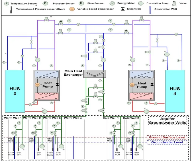
Each well in the ATES system is installed in an underground concrete structure (small room) accessible by a ladder. The concrete structures (rooms) are linked with each other and with the pumps control room by underground pipes. These pipes are used as connection paths for signal and electric cables linking different components installed in the wells with the control room in the building garage. Each well room consists of a pumping and an observation well. Each observation well is equipped with a submerged diver of type STS ATM/N/T DMM029 that measures both the temperature and water level. The diver has a measuring range and accuracy of -25 to 80 ± 1°C and up to 25 ± 0.25% bars. Each pumping well is equipped with a pump of type GRUNDFOS SP 46-4-C for warm wells and GRUNDFOS SP 60-4 for cold wells, as well as a pressure sensor (Siemens QBE2103-P4) and temperature sensor (Siemens QAE2121.010) measuring range and accuracy of up to 4 ± 0.1% bars and -30 to 130 ±0.5°C respectively. The latter sensors are installed on the main pipe just outside the well. All wells on each side (warm and cold) are grouped into one main supply pipe to extend towards the building. The building is equipped with a secondary heat exchanger that separates the ground water loop and the heat pump secondary fluid loop to avoid clogging in the evaporator of the heat pump. Energy meters (Siemens Sitrans F M MAG 5000 & Siemens QAE21) are installed on both sides of the secondary heat exchanger to monitor energy exchange between the ATES and buildings (see Figure 1).
ATES Operation in brief
Heating Mode: The wells are used in injecting or extracting mode depending on the season. During the
down through heat exchange with the building. Heating is done with the assistance of the heat pumps. If the temperature in the warm wells drop below a pre-defined set point, the heating is supplied through district heating network.
Cooling Mode: Throughout the heating season, cold storage is being accumulated. During the summer, the
cycle is reversed and free cooling is utilized. Water from the cold side of the ATES is extracted and re-injected in the warm side after being heated up through heat exchange with the building. If the temperature in the cold wells exceeds a pre-defined set point, the cooling is supplied with the assistance of the heat pumps. During the cooling season, occasional heating loads as well as heat for domestic hot water is provided by district heating network (see figure 1). Distributed temperature measurements
Two continuous fiber optical cables have been installed in each side of the ATES wells groups. Each cable consists of four fibers two of which are used. Each cable is connected from both sides to the DTS equipment to enable both single and double-ended connection configuration. Along each cable, four sections of the fiber cable are coiled in the beginning, middle and the end of the cable to be used for calibration. The fiber cables are connected to two distributed temperature sensing instruments HALO and SILIXA XT with sampling resolution of 2 and 0.25 m, respectively (see figure 2). The former instrument was used only temporarily while the latter is installed for permanent measurements. Some SILIXA XT data is presented in this paper. Two additional PT100 resistance thermometers with accuracy of ±0.005°C are connected to the DTS and used to provide dynamic measurements of the calibration baths near the DTS. Physical principle used in the DTS equipment is based on the glass fibers sensitivity to temperature change. The DTS equipment sends a laser beam through the fiber and collects the back-scattered signal and translate it into temperature (Suárez et al., 2011). The temperature received from the DTS is averaged over both space and time. The temporal and spatial sampling resolutions of the DTS instrument are set to be 10 minutes and 0.25 m respectively. The DTS has four channels. The first and second channels are connected to the fiber cable installed in cold side. The third and forth channels are connected to the fiber cable installed in warm side (see figure 2). The laser beam is sent from one channel at a time. Therefore, each channel integrates and records the temperatures once every 40 minutes. Since the cable installation was continuous, additional splices along the cable were avoided (except one splice in the beginning of the cable to connect it to the DTS). This significantly avoids the risk of local losses along the fiber cable and make the calibration procedure less complex and temperature measurements more reliable. Channel 1 and 2 (in XT Silixa DTS) are measuring the cold side using the same fiber cable but two different fibers within the cables. The same has been done for channel 3 and 4 (in XT Silixa DTS) on the warm side.
DTS Calibration: the DTS measurement setting used is single ended mode with dynamic calibration using two matching sections in the same bath at the beginning and the end of the fiber cable (Hausner et al., 2011). The DTS equipment is calibrated using equation 1. Where at position z (in m) along the fiber cable length, PS(z), PaS(z) and T(z) are the signal strength of the Raman-Stokes, Raman-AntiStokes and the temperature at that position, respectively. Additionally, γ (in Kelvin) represents the energy shift between the incident and scattered photon. C is a dimensionless parameter to take into account and calibrate the local losses. These local losses occur in connectors and fiber splices. ∆α (in m-1) is the differential attenuation in the fiber along the fiber cable.
Figure 1 Schematic diagrams that shows the wells in ATES, heat pump and their connection to the building
Figure 2 Schematic diagrams that shows the fiber cable installation in warm and cold wells in ATES and channel connections
(1)
The first and fourth calibration coils, for each the warm and cold side, (at the beginning and the end of the cable) are placed in the same calibration bath and used to calibrate ∆α. Cinternal (loss inside the DTS instrument) is calibrated using the default ∆αinternal given by the instrument as well as the values for γ , PS(z), PaS(z) and T(z) also given by the instrument for the internal reference section. Cinternal is then averaged over the internal section. The average value of Cinternal, ∆αinternal, γ, and T(z) measured by the thermometer PT100 in the first calibration bath located near the DTS are used to calibrate Cexternal.Cexternal accounts for Cinternal, Cconnector and Csplice combined. Cconnector and Csplice refer to the local loss due connecting the fiber cable to the DTS and connecting (splicing) the fibers in the red fiber cable with the fibers in the yellow fiber cable (see figure2). Since the fiber cable is continuous through out the installation, additional splices were avoided and Cexternal is used to calculate the temperature along the rest of the cable. Cexternal is assumed to be constant for each time step. All ∆α, and C parameters are calibrated dynamically for each time step. In the other hand, γ and ∆αinteranl is assumed to be constant and default values provided by the manufacture were used. The temperature measurements are validated with the third fiber coil (see figure 2) placed in a validation bath located approximately in the middle of the fiber cable. The calibration and validation process has been conducted over two weeks. The maximum and average deviation achieved between the validation bath temperature and the measured temperature by the DTS are -0.19°C and ± 0.09°C respectively. FIRST MEASUREMENT
The ATES system has been monitored since March 2016 mainly using water level and temperature sensors and flowmeters. The ATES started operation in the fall of 2016. The fiber optical cables and DTS were installed and started the measurement in the fall of 2017. During the first heating and cooling season October 2016 - September 2017, the total heating and cooling energy consumed from the Aquifer are 189 MWh and 235 MWh respectively. Since the beginning of the second heating season in October 2017 and until March 2018, 147 MWh of total energy was utilized from the ATES the majority of which (143 kWh) for heating.
Power Measurement
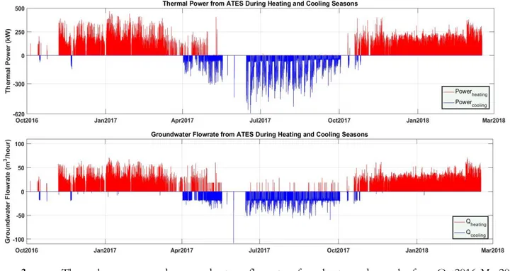
Since March 2016, the maximum heating and cooling power used are 469 kW and 610.5 kW respectively. The average groundwater flow utilized throughout the heating and cooling seasons are around 26 m3/hour and 21
m3/hour respectively. This accounts for no more than 15% of the allowed pumping flow rate. Figure 3 shows the
power (upper side of the figure) and groundwater flow rate (lower side of the figure) during the period October 2017- March 2018. The positive red lines indicate power and flow rate measurements in heating mode while the negative blue ones indicate power and groundwater flow measurement during cooling.
Similarly, figure 4 shows the extraction and injection temperatures for both heating and cooling mode during the period October 2017- March 2018. The red dots indicate extraction and injection temperatures measurement in heating mode while blue dots indicate extraction and injection temperatures measurement in cooling mode. The values presented in figure 3 and figure 4 are measured at the inlet and the outlet of the main heat exchanger (called additional heat exchanger in figure 1) between the ATES the building.
Figure 3 Thermal power and groundwater flowrate for heat and cool for Oct2016-Mar2018
Figure 4 Extraction and injection temperatures for heating and cooling during Oct2016-Mar2018 DTS TEMPERATURE MEASUREMENT
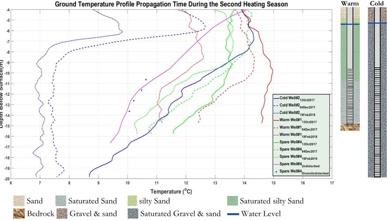
The DTS measurements provided a good insight into the temperature profile with depth as well as the temperature propagation through the ATES. Figure 5 shows the temperature measurements from the fiber cable installed in the observation wells of cold well number two and warm well1 number one as well as the spare pumping
well. The measurements are presented at three different time steps: at the beginning, near the end and during the second heating season of the ATES. Cold well number two and warm well number one are located about 120 m apart at the far end of each side of the ATES. The spare well is located in between them with a distance of approximately 40 m from warm well number one. The negative sign on the y-axis in figure 5 indicate depth below ground surface. The water level in each well is ranging between -2 and -5 m depending on injection or extraction operation. The screen of each well starts at depth -9 m. The well screen depths are 7, 5 and 9 m for the warm, spare and cold wells respectively. Each one of the wells in figure 5 is represented by three lines. The solid, dashed and dotted lines represent measurement dates on 13th Oct 2017, 04th Dec 2017 and 19th Feb 2018 during the beginning, middle and
near the end of the heating season. Furthermore, the undisturbed ground temperature profile before ATES started the operation measured on 26th August 2016 is presented in figure 5. The purple solid line shows measured temperature
using Oryx DTS (1 m sampling resolution). The blue circles are measurements using divers at several depths within the well filter.
ATES PERFORMANCE EVALUATION
For ATES performance evaluation, energy balance (EB), hydraulic recovery (HR) and thermal recovery (TR) are used as ATES performance indicators.. EB is defined as the net energy utilized during heating or cooling divided by the total amount used for one full season of both heating and cooling. EB values ranges between -1 and 1. A value of 0 indicates a balanced system over the year. HR is defined as the ratio of water volume utilized during one heating or cooling season divided by water volume used in its preceding heating or cooling season during 12 contentious months. TR is defined as the ratio between the thermal energy extracted in one heating or cooling season divided by the thermal energy injected to ATES during its preceding heating or cooling season during 12 contentious months. HR or TR value of 1 indicates the all the water volume or the thermal energy injected in the previous season has been fully extracted (recovered). TR and HR for the first cooling season are estimated around 0.33 and 1.37 respectively. EB of the first full heating and cooling season is 0.12.
Warm Cold
Sand Saturated Sand silty Sand Saturated silty Sand Bedrock Gravel & sand Saturated Gravel & sand Water Level
DISCUSSION AND CONCLUSION
The high hydraulic conductivity and high allowable injection and extraction flowrates, as well as the hydrogeological conditions of a site in Stockholm, Sweden, have been favorable for an ATES system. The real state property is located on top of an Esker formation with a core mostly consisting of gravel and sand. A monitoring set up of the ATES consisting of temperature, pressure and flow meters has been connected to the building control system.
Additionally, for monitoring, a XT Silixa DTS with sampling resolution of 0.25 m and continuous fiber optical cables have been installed in all pumping and some observation wells. DTS is dynamically calibrated using three calibration baths in the beginning and the end of each cable. The DTS temperature measurements are controlled using a bath in the middle of each fiber cable. The maximum and average deviation recorded by the DTS in the temperature measurement when compared to the validation bath are - 0.19°C and ± 0.09°C respectively. These numbers may be improved by mixing the calibration baths temperatures. Proper calibration of the DTS is critical to measure with sufficient accuracy for ATES applications. Therefore, DTS equipment dynamic calibration of signal losses due to length and local effects a recommended.
Traditional local in-well measurement instruments such as divers can be misleading when it comes to temperature. During the cooling season, the building control system is supposed to automatically operate on free cooling mode as long as the temperature in the ATES is low enough. In June 2017, a diver controlling the operation recorded too high temperatures (13°C), and thus the ATES stopped working in free cooling mode. In reality, the temperature in the ATES was suitable (6°C) to operate on free cooling mode as shown by the DTS. The reason behind this was due to diver misplacement since it is located too high in the well and next to the pump.
The highest extraction temperature for the first and second heating season are 14.9°C and 16.3°C and the lowest temperatures are 7.6°C and 10.8°C respectively. The highest and lowest extraction temperature for the first cooling season are 12.1 and 5.4°C, respectively. The average temperature difference between extraction and injection pipe for the first and second heating season are 3.7°C and 3.9°C, respectively, while the average temperature difference for the cooling season is 5°C. Near the end of the cooling season (after mid-August), the extraction temperatures are exceeding average undisturbed temperature (10.7°C) in the aquifer (average temperature along well depth starting at the groundwater water level). This is an indication of thermal break through. The hydraulic recovery value of 1.37 for the first cooling season indicates that more water volume was used during the cooling season than in the first heating season. The storage volume extracted from the warm storage during the first heating season and injected into the cold storage was 36900m3/year. The storage volume recovered for cooling during the cooling season is 50500m3/year and
thus the imbalanced value of HR. This imbalance resulted in water from the warm storage reaching the cold storage (thermal breakthrough). During the summer and before the cooling season ended (mid-August), all the water that was injected in the previous season was recovered and the temperature of the ground return to the undisturbed condition. However, since additional cooling was done until the end of the cooling season (September), the warm water injected in the warm side during the cooling season started to move towards the cold side and eventually reached the cold storage side of the aquifer.
The temperature profile of the cold well in October (end of cooling season) shown in figure 5, shows a sign of thermal break through with temperature values exceeding 13.0°C. It also shows a tilted thermal front with a temperature gradient over the filter depth with 13.3°C at the top and 8.7°C at the bottom. This can likely be due to buoyancy flow caused by the difference in water density between the injected-extracted water and the ambient groundwater density. The shape of the profile is probably also affected by the undisturbed temperature profile. Additionally, pump placement just above the filter section would potentially cause higher inflow rates at the top of the filter than the bottom (Houben & Hauschild, 2011). This could result in a velocity profile along the filter depth having higher velocity at the top of the well screen than the bottom (considering similar sediment, hydraulic conductivity and well screen spacing). Therefore, in addition to aiming for a balance ATES, pump placement optimization can be further investigated. For instance, by lowering the pump at the middle of the filter section, it would potentially result in a more even inflow distribution along the well screen thus reducing the thermal front tilting angle.
Despite the fact that more water volume was recovered in the summer than injected in the preceding winter, the thermal recovery for first cooling season is calculated to be 33% of the total energy injected in the previous heating seasons. When it comes to energy balance over the first heating and cooling season, EB value of 0.12 indicates
a net heating of the ATES over the first year. From an individual ATES system stands point, it is beneficial to increase the storage volume. On the other hand, this can also limit the construction of other ATES systems in its vicinity. If such plans are made, careful consideration and coordination with the existing ATES system is necessary. For instance, installing wells with the same type of storage (warm or cold) in the same area. This can enhance the thermal recovery, as the storage volume will increase.
ACKNOWLEDGMENTS
Special thanks to the Swedish Energy Agency and Effsys Expand research program for funding this project. Additionally, our gratitude is extended to our partners for their support to make this work possible: Alverdens, AMF Fastigheter, Asplan Viak, Atlas Copco, AVANTI, Bengt Dahlgren, Cooly AB, Danfoss Heat Pumps, Finspångs Brunnsborrning, HP Borrningar, Geobatteri, Geostrata HB, NGU, NIBE, Nowab, NTNU, Palne Mogensen AB, Stures Brunnsborrningar, SGU, SLU, SWECO, Vasakronan, Värmex, Wilo Sweden AB and WSP.
NOMENCLATURE
PS = Raman-Stokes (nm)
PaS = Raman-AntiStokes (nm)
T = Temperature (°C)
z = Position along the fiber cable (m)
γ = Energy shift between the incident and scattered photon (K) ∆α = Differential attenuation along the fiber cable (m-1)
C = Dimensionless parameter for local losses calibration (-) Subscripts
internal = Internal reference section in the DTS connector = Connector between DTS and fiber cable splice = connection (welding) between two fiber cable
external = Refers to the rest of the fiber cable after the splice
REFERENCES
Bakr, M., van Oostrom, N., & Sommer, W. (2013). Efficiency of and interference among multiple Aquifer Thermal Energy Storage systems; A Dutch case study. Renewable Energy, 60(Supplement C), 53–62.
https://doi.org/10.1016/j.renene.2013.04.004
Bloemendal, M., & Hartog, N. (2018). Analysis of the impact of storage conditions on the thermal recovery efficiency of low-temperature ATES systems. Geothermics, 71, 306–319.
Boman, D., & Hanson, G. (2004). Salt grundvatten i Stockholms läns kust- och skärgårdsområden: metodik för
miljöövervakning och undersökningsresultat 2003. Länsstyrelsen i Stockholms län. Retrieved from
http://www.diva-portal.org/smash/record.jsf?pid=diva2:851965
Hausner, M. B., Suárez, F., Glander, K. E., Giesen, N. van de, Selker, J. S., & Tyler, S. W. (2011). Calibrating Single-Ended Fiber-Optic Raman Spectra Distributed Temperature Sensing Data. Sensors, 11(11), 10859–10879.
https://doi.org/10.3390/s111110859
Houben, G. J., & Hauschild, S. (2011). Numerical Modeling of the Near-Field Hydraulics of Water Wells. Ground Water,
49(4), 570–575. https://doi.org/10.1111/j.1745-6584.2010.00760.x
Lee, K. S. (2010). A Review on Concepts, Applications, and Models of Aquifer Thermal Energy Storage Systems.
Energies, 3(6), 1320–1334. https://doi.org/10.3390/en3061320
Lee, K. S. (2013). Aquifer Thermal Energy Storage. In Underground Thermal Energy Storage (pp. 59–93). Springer, London. https://doi.org/10.1007/978-1-4471-4273-7_4
Molz, F. J., Melville, J. G., Parr, A. D., King, D. A., & Hopf, M. T. (1983). Aquifer thermal energy storage : A well doublet experiment at increased temperatures. Water Resources Research, 19(1), 149–160.
https://doi.org/10.1029/WR019i001p00149
Molz, F. J., Parr, A. D., & Andersen, P. F. (1981). Thermal energy storage in a confined aquifer: Second cycle. Water
Resources Research, 17(3), 641–645. https://doi.org/10.1029/WR017i003p00641
Possemiers, M. (2014). Influence of Aquifer Thermal Energy Storage on groundwater quality: A review illustrated by seven case studies from Belgium. Journal of Hydrology: Regional Studies, 2(Supplement C), 20–34.
https://doi.org/10.1016/j.ejrh.2014.08.001
Regeringskansliet, R. och. (2017, April 27). Övergripande mål och svenska mål inom Europa 2020 [Text]. Retrieved October 24, 2017, from http://www.regeringen.se/sverige-i-eu/europa-2020-strategin/overgripande-mal-och-sveriges-nationella-mal/
Sauty, J. P., Gringarten, A. C., Fabris, H., Thiery, D., Menjoz, A., & Landel, P. A. (1982). Sensible energy storage in aquifers: 2. Field experiments and comparison with theoretical results. Water Resources Research, 18(2), 253–265. https://doi.org/10.1029/WR018i002p00253
Sommer, W. (2015). Modelling and monitoring of Aquifer Thermal Energy Storage: Impacts of heterogeneity, thermal
interference and bioremediation.pdf (PhD thesis). Wageningen University, Wageningen, Netherlands.
Retrieved from http://library.wur.nl/WebQuery/wurpubs/fulltext/342495
Sommer, W. T., Doornenbal, P. J., Drijver, B. C., Gaans, P. F. M. van, Leusbrock, I., Grotenhuis, J. T. C., & Rijnaarts, H. H. M. (2014). Thermal performance and heat transport in aquifer thermal energy storage. Hydrogeology
Journal, 22(1), 263–279. https://doi.org/10.1007/s10040-013-1066-0
Suárez, F., Aravena, J. E., Hausner, M. B., Childress, A. E., & Tyler, S. W. (2011). Assessment of a vertical high-resolution distributed-temperature-sensing system in a shallow thermohaline environment. Hydrology and
Earth System Sciences; Katlenburg-Lindau, 15(3), 1081.
Sundberg, J. (1991). Termiska egenskaper i jord och berg (p. 18). Linköping: Swedish geotechnical institute. Retrieved from http://www.swedgeo.se/globalassets/publikationer/info/pdf/sgi-i12.pdf
Svedinger, B. (1981). Värme i jord, berg och vatten : utvinning och lagring. Stockholm: Statens råd för byggnadsforskning :
Swdish Energy Agency. (2015). Energy Outlook. Retrieved October 24, 2017, from
https://www.energimyndigheten.se/contentassets/50a0c7046ce54aa88e0151796950ba0a/energilaget-2015_webb.pdf
United Nations. (2015). Paris Agreement. Retrieved from
http://unfccc.int/files/essential_background/convention/application/pdf/english_paris_agreement.pdf Visser, P. W., Kooi, H., & Stuyfzand, P. J. (2015). The thermal impact of aquifer thermal energy storage (ATES) systems:
a case study in the Netherlands, combining monitoring and modeling. Hydrogeology Journal, 23(3), 507–532. https://doi.org/10.1007/s10040-014-1224-z
WSP. (2014). Miljökonsekvensbeskrivning: akvifärlager Rosenborg 3, Solna stad. Ansökan om tillstånd för vattenverksamhet. Retrieved October 24, 2017, from