Estimating soil salinity from remote sensing data in corn fields
12
0
0
Full text
(2) Eldiery et al.. salinization, is the result of salt stored in the soil profile being mobilized by extra water provided by human activities such as irrigation (Szabolcs 1989). The Arkansas River is one of the most saline rivers of its size in the United States. Salinity levels, measured as dissolved solid concentrations, increase from 300 mg/L near Pueblo to over 4,000 mg/L at the ColoradoKansas border (Ghassemi et al. 1995). It was estimated that in 1977 over 200,000 acres in the Arkansas Valley were being irrigated with water that contained salinity concentrations greater than 1,400 mg/L (Miles 1977). Gates et al. (2002) established that salts were returned from the irrigated valley to the Arkansas River at an estimated average rate of about 740 kg/week per irrigated hectare. Goff et al. (1997) noted that the degradation of the quality of surface and groundwater in the lower Arkansas River Valley is closely related to extensive agricultural diversions and usage, and the consumption of irrigation water by evapotranspiration increases salinity in return flows. Remotely sensed data has a great potential for monitoring dynamic processes, including salinization. The ability to predict soil salinity accurately from remote sensing data is important because it saves labor, time, and effort when compared to field collection of soil salinity data (Robbins and Wiegand 1990). Remote sensing of surface features with aerial photography, videography, infrared thermometry, and multispectral scanners has been used intensively to identify and map salt-affected areas (Robbins and Wiegand 1990). Metternicht and Zinck (1997) combined digital image classification with field observation of soil degradation and laboratory analysis to map salt and sodium-affected areas in the semiarid valleys of Cochabamba, Bolivia. Multispectral data acquired from platforms such as Landsat, SPOT, and the Indian Remote Sensing (IRS) series of satellites, have been found to be useful in detecting, mapping and monitoring salt affected soils. Dwivedi and Rao (1992) noted that the digital analysis of multispectral data using the spectral response pattern of salt-affected soils is plagued by misclassification, and in order to improve the detectability of these soils and other natural features using remote sensing data various image transforms must be developed. These transforms not only enhance the detectability of these features, but also aid data compression resulting in substantially reduced computational time and cost (Dwivedi and Rao 1992). Band ratios of visible to near-infrared and between infrared bands have proven to be better for identifying salts in soils and salt-stressed crops than individual bands (Craig et al. 1998; Hick and Russell 1990; and Hick et al. 1984). Srivastava et al. (1997) studied the accuracy of mapping shallow groundwater depth and salinity using remote sensing data. They formulated a methodology involving image processing and GIS techniques using false color, vegetation indices, density slicing, overlaying, and supervised classification and applied the methodology to IRS-1B LISSS II data. In their study, groundwater depth and salinity maps were based on reflectance variations of vegetation above the ground surface, and they assert that the species of vegetation found in an area and vegetation densities can provide evidence of shallow groundwater conditions. Wiegand et al. (1994) assessed the extent and severity of soil salinity in fields in terms 32.
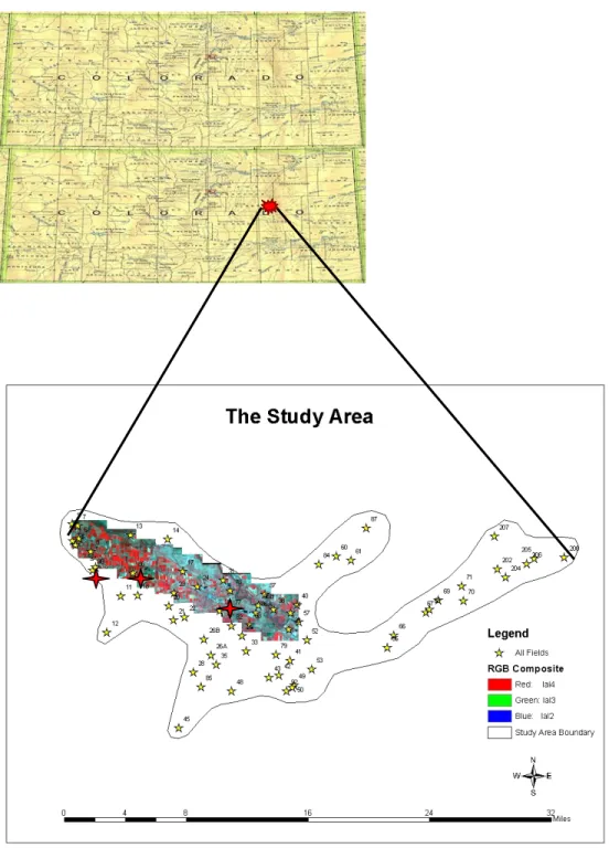
(3) Estimating soil salinity from remote sensing data. of economic impact on crop production and effectiveness of reclamation efforts. Their study emphazised practical ways of combining image analysis capabilities, spectral observations, and ground truth to map and quantify the severity of soil salinity and its effects on crops. Golovina et al. (1992) made an effort to automate methods of interpreting aerial photos in order to speed up the interpretation process and make it more objective. They stated that automated analysis is capable of performing a more complex evaluation of the quantitative degree of salinization than visual interpretation. The integration of remotely sensed data, Geographic Information Systems (GIS), and spatial statistics provides useful tools for modeling variability to predict the distribution, presence, and pattern of soil characteristics (Kalkhan et al. 2000). This integration also provides tools for assessing the landscapescale structure of forest and rangelands (Chong et al. 2001). Kalkhan et al. (2000) incorporated trend surface analysis to estimate the probability of exotic species richness. They found that Landsat TM bands 1, 2, 5, 6, and 7, elevation, slope, and aspect were significant predictors. Thomas et al. (1997) presented a rapid, cost-efficient methodology to link plant diversity surveys from plots to landscapes using unbiased site selection based on remotely sensed information. Utset et al. (1998) used a calibrated Four-Electrode Probe (FEP) for inexpensive and indirect determinations of salinity-sensor electrical conductivity (EC) in a plot in Cauto Valley, Cuba. Their crossvalidation analysis showed that EC semivariograms obtained from FEP measurements can characterize the soil EC spatial variation in a similar way to semivariograms of laboratory-measured soil EC. In this paper, we evaluate the relationship between soil salinity and satellite imagery. These relationships are evaluated using multiple regression models that are capable of accounting for any spatial dependency in the residuals. The best model is then used to produce salinity maps.. 2. Site Description and Data Collection The study area (Figure 1) for this project is located in southeastern Colorado, primarily in Otero County. This region was selected because it provides a good illustration of a salinity-affected area. The salinity monitoring program is applied on the sub-region scale and on the field scale. For the sub-region scale, salinity readings are taken twice each growing season in approximately 69 fields with an EM-38 salinity probe (Gates et al. 2002). This EM-38 data is collected at between 60 and 120 points in each field depending on the field's area. In each of these fields, there is one monitoring well where groundwater level and groundwater salinity readings are taken during the year. For the field scale, fields with different irrigation systems, soil types and crop types were selected. In each of these fields, salinity readings are taken three times during the growing season. Each field also contains between 7 and 15 monitoring wells. At the field scale, the following readings are taken: soil salinity, water table fluctuation, and groundwater salinity, rainfall, estimates of irrigation water quality and quantity, and evapotranspiration. Yield samples are also taken. Figure 1 shows the map of the study site along with the Ikonos satellite imagery that 33.
(4) Eldiery et al.. was acquired in 2001. The image covers part of the study area. The dominant irrigated fields were alfalfa, corn, cantaloupe, and onion. Five fields were selected for field scale study (7, 17, 20, 40 and 80). Three of these fields were planted with corn (17, 40, and 80) and are described in this paper. The other two fields (7 and 20) are excluded from this discussion because field 7 was planted with alfalfa and field 20 was not covered by the image.. Figure 1. Map of the Lower Arkansas Valley study area.. 34.
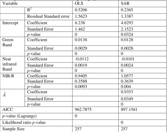
(5) Estimating soil salinity from remote sensing data. 3. Methodology and Procedure A satellite image from Ikonos was taken in 2001 which covers a part of the study area where the field scale monitoring is taking place. The irrigated fields in this region are mainly alfalfa, corn, wheat, cantaloupe, and onion. The reflection of the satellite image is affected mainly by the ground cover type, and each crop has a different reflection. For, the study described in this paper, only fields planted with corn (17, 40, and 80) were used. Soil salinity data collected using the EM-38 salinity probe are tied by location to the corresponding values from the different bands of the Ikonos satellite image. The stepwise regression technique is used to decide the combination of variables from the Ikonos image bands that relate to soil salinity. The relationships between soil salinity data and the four bands of the Ikonos satellite image (blue, green, red, and near infrared), the normalized difference vegetation index (NDVI), the near infrared band divided by red band (NIR/R), and principal component analysis (PCA) are evaluated with the regression models. The residuals from the regression models were tested for spatial autocorrelation using Moran’s I and the Lagrange multiplier test. In analyzing the residuals inverse distance weighting was used to define the spatial proximity of the sample data. If the residuals showed signs of spatial autocorrelation, the model was refit using a spatial autoregressive model (SAR). A likelihood ratio test was used to test the improvement of the SAR model to that of the ordinary least squares (OLS). Competing models were evaluated using Akaike Information Corrected Criteria (AICC).. 4. Results and Analysis Table 1 summarizes the results of the analysis. The OLS model included the green band, the near infrared band, and near infrared band divided by red band (NIR/R). The green band and NIR/R band ratio had a positive relationship with soil salinity while the near infrared band had a negative relationship. Analysis of residuals suggested that there might be some spatial dependency based on the Lagrange multiplier test. To account for the spatial dependency, the same variables were also presented to the SAR model, however their level of significant was lower. The likelihood ratio test indicated that the SAR model was a significant improvement over the OLS model. Also, the AICC for the SAR was smaller than that for the OLS model. ∧ There was a significant amount of spatial autocorrelation in the residuals ( λ. = 0.93). This explains the decrease in the R2 value for the SAR model when compared to the OLS model (0.24 vs. 0.52). The presence of spatial autocorrelation makes the relationship between the satellite imagery and soil salinity more important than it actually is, thus inflating the R2 value as well as deceasing the standard errors associated with the parameter estimates.. 35.
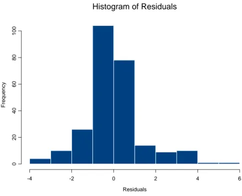
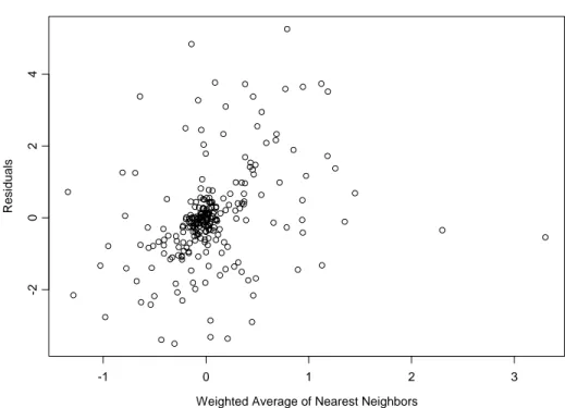
(6) Eldiery et al.. Table 1. Summary of statistics for the OLS and SAR models for predicting soil salinity as a function of remote sensing imagery. Variable 2. Intercept. Green Band Near infrared Band NIR/R. ∧. λ. R Residual Standard error Coefficient Standard Error p-value Coefficient Standard Error p-value Coefficient Standard Error p-value Coefficient Standard Error p-value Coefficient. OLS 0.5206 1.5623 6.238 1.462 0 0.0136. SAR 0.2365 1.3387 4.6293 2.1523 0.0324 0.0128. 0.0029 0 -0.0112 0.0019 0 0.9405 0.3588 0.0093. 0.0028 0 -0.0101 0.0024 0 1.0577 0.3639 0.004 0.9353. Standard Error p-value. AICC p-value (Lagrange) Likelihood ratio p-value Sample Size. 962.7875 0 257. 0.0349 0 897.1561 0 257. Analysis of the residuals from the SAR model are displayed in figures 2,3 and 4. The residuals are approximately normally distributed as is clear from Figure 2. The errors associated with the predicted soil salinity increased with increasing value of soil salinity values as seen in Figure 3. Finally, in the plot of residuals versus a weighted average of nearest neighbors (Figure 4), no pattern exists, suggesting that the SAR was able to account for the spatial dependency in the residuals.. 36.
(7) Estimating soil salinity from remote sensing data. 60 0. 20. 40. Frequency. 80. 100. Histogram of Residuals. -4. -2. 0. 2. 4. 6. Residuals. Figure 2. Histogram of residuals.. -2. 0. Residuals. 2. 4. Residuals vs Predicted Soil Salinity. 3. 4. 5. 6. 7. Predicted Soil Salinity. Figure 3. Residuals versus predicted values of soil salinity.. 37. 8. 9.
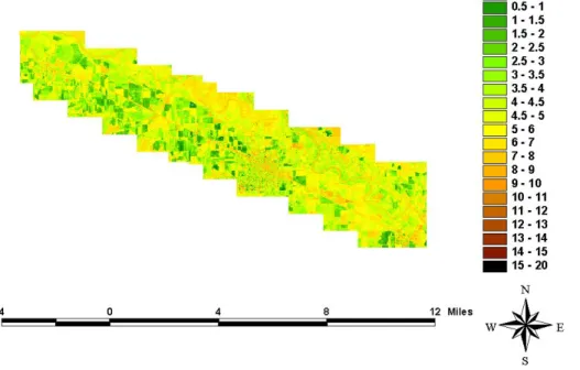
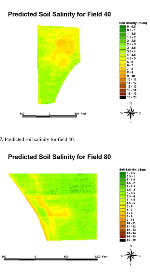
(8) Eldiery et al.. -2. 0. Residuals. 2. 4. Residuals vs Weighted Average of Nearest Neighbors. -1. 0. 1. 2. 3. Weighted Average of Nearest Neighbors. Figure 4. Residuals versus the weighted average of nearest neighbors. The following figures (5, 6, 7, and 8) show the predicted soil salinity maps for the area covered by the image and another three corn fields. These maps are derived using the equation for the SAR model shown in Table 1. Figure 5 represents the whole area covered by the image. In addition to the irrigated fields, this area contains many other non-irrigated areas (rivers, lakes, urban areas, etc). The soil salinity values for these non-irrigated areas are not realistic since there were no data collected for these areas. But when looking at the fields where data were collected, especially for the images of the individual fields, the non-irrigated areas help in interpreting the results. Field 17 represents one of the homogeneous fields, except for a small area at the left north part of the field, the field's salinity level is almost the same throughout. This homogeneity is reflected in the predicted soil salinity map shown in Figure 6. Field 40 and field 80 represent heterogeneous fields. The predicted maps for these two fields (Figures 7 and 8) show most of the highly affected areas by soil salinity.. 38.
(9) Estimating soil salinity from remote sensing data. Figure 5. Predicted soil salinity for the area covered by the image.. Figure 6. Predicted soil salinity for field 17.. 39.
(10) Eldiery et al.. Figure 7. Predicted soil salinity for field 40.. Figure 8. Predicted soil salinity for field 80.. 40.
(11) Estimating soil salinity from remote sensing data. 5. Summary and Conclusion The results presented in this paper show the feasibility of using remote sensing data to predict soil salinity. Compared to the labor, time, and money invested in field work devoted to collecting soil salinity data, the availability and ease of acquiring satellite imagery is very attractive. Numerous combinations of bands have been evaluated using OLS and SAR models. It is clear from the results presented in this paper that selecting the regression model is very important in determining the quality of the map of predicted soil salinity. The results also show the importance of the residuals and how they can affect the quality of the maps generated. The presence of spatial autocorrelation makes the relationship between the satellite imagery and soil salinity more important than it actually is. In evaluating the regression techniques for soil salinity, attention should be paid to the issue of selecting the most suitable regression model. It is very important for future research to consider most of the regression variables that control the accuracy of the regression. This paper shows that depending only on R2 and standard errors will not produce salinity maps of high quality and high accuracy when using remote sensing. Likelihood ratio test, Lagrange multiplier, and AICC must be considered to improve the quality of the interpolated maps.. References Chong, G.W., Reich, R.M., Kalkhan, M.A., and Stohlgren, T.J. (2001). “New approaches for sampling and modeling native and exotic plant species richness.” Western North American Naturalist, 61, 328-335. Craig, J. C., Shih, S. F., Boman, B. J., & Carter, G. A. (1998). Detection of salinity stress in citrus trees using narrow-band multispectral imaging. ASAE paper no. 983076. ASAE Annual International Meeting, Orlando, FL, USA, 12–16 July 1998. 10 pp. Dwivedi, R.S., and Rao, B.R.M., (1992). “The selection of the best possible Landsat TM band combination for delineating salt-affected soils.” International Journal of Remote Sensing, 13, 2051–2058. Ghassemi, F., Jackeman, A.J., and Nix, H.A. (1995). Salinization of land and water resources: human causes, extent, management and case studies. CAB International, Wallingford Oxon, UK. Gates, T.K., Burkhalter, J.P., Labadie, J.W., Valliant, J.C, and Broner, I., (2002). “Monitoring and Modeling Flow and Salt Transport in a Salinity-Threatened Irrigated Valley.” Journal of Irrigation and Drainage Engineering. March / April 87-99. Goff, K., Michael, E.L, Mark, A. P., and Leonard, F. K., (1998). “Simulated Effects of Irrigation on Salinity in the Arkansas River Valley in Colorado.” Groundwater Golovina, N.N., Minskiy, D.Ye., Pankova, I., and Solov’yev, D.A. (1992). “Automated air photo interpretation in the mapping of soil salinization in cottongrowing zones.” Mapping Sciences and Remote Sensing, 29, 262-268. Hick, P.T., and Russell, W.G.R. (1990). “Some spectral considerations for remote sensing of soil salinity.” Australian Journal of Soil Research, 28, 417–431.. 41.
(12) Eldiery et al.. Hick, P.T., Davies, J.R., and Steckis, R.A. (1984). “Mapping dryland salinity in Western Australia using remotely sensed data.” Satellite remote sensing: review and preview, Remote Sensing Society, Reading, UK, 343–350. Hillel, D. (2000). “Salinity management for sustainable irrigation: integrating science, environment, and economics.” The World Bank: Washington D.C. Kalkhan, M. A., Stohlgren, T. J., Chong, G. W., Lisa, D., and Reich, R. M. (2000). “A predictive spatial model of plant diversity: integration of remotely sensed data, GIS, and spatial statistics” Paper presented at the Eighth Biennial Remote Sensing Application Conference (RS 2000), April 10-14, 2000, Albuquerque, NM. Metternicht, G.I. and Zinck, J.A. (1997). “Spatial discrimination of salt- and sodium-affected soil surfaces.” International Journal of Remote Sensing, 18, 2571–2586. Miles, D.L. (1977). “Salinity in the Arkansas Valley of Colorado. U.S. Environmental Protection Agency,” Interagency Agreement, Colorado State University, EPA-1AG-D4-0544, Fort Collins, CO. Postel, S. (1999). Pillar of Sand: Can the Irrigation Miracle Last? W.W. Norton and Co., New York, NY. Robbins, C.W., and Wiegand, C.L. (1990). “Field and laboratory measurements.” Agricultural Salinity Assessment and Management, American Society of Civil Engineers, New York. Srivastava, A., Tripathi N. K., and Gokhale, K. V. G. K. (1997). "Mapping groundwater salinity using IRS-1B LISS II data and GIS techniques." International Journal of Remote Sensing, 18 (13), 2853-2862 Szabolcs, I. (1989). Salt-Affected Soils. CRC Press, Boca Raton, FL. Thomas J.S., Geneva W.C., Khalkhan M.A., and Lisa D.S. (1997). “Multiscale sampling of plant diversity: effects of minimum mapping unit size.” Ecological Application, 7(3), 1064-1074 Utset, A., Ruiz, M., Herrera, J. and Deleon, D. 1998. “A geostatistical method for soil salinity sample site spacing.” Geoderma, 86, 143–151. Wiegand, C.L., Rhoades, J.D., Escobar, D.E., and Everitt, J.H. (1994). “Photographic and videographic observations for determining and mapping the response of cotton to soil salinity.” Remote Sensing of Environment, 49, 212-223.. 42.
(13)
Figure
+3
Related documents
Denna studie syftar till att undersöka hur akademitränare ser på talang hos unga fotbollsspelare och visar på att tränarna tycker att talang är svårt att definiera men att
The following inclusion criteria will be applied in the search: (a) the articles have to address peer assessment in higher education; (b) focusing formative peer assess- ment;
När barn möter motstånd till att ansluta till pågående aktiviteter utvecklar de komplexa tillträdesstrategier (Corsaro 2015, s. Det som framträder i denna studien är ett
Företag 1 använder sig av en finansmanual, där det står vilka kriterier som ska uppfyllas för att aktivering ska vara möjlig. Manualen är något tydligare än punkt 57 IAS 38 och
We found limited to moderate evidence that for adults who seek out this treatment, therapist- guided I-CBT has a favorable short-term effect compared to waiting list for social
Hay meadows and natural pastures are landscapes that tell of a time when mankind sup- ported itself without artificial fertilisers, fossil fuels and cultivated
Moreover, three scenarios of rainfall were used to calculate the R factor in the RUSLE and these scenarios were derived from the Swedish Meteorological and Hydrological
The 2014 anomaly can be seen at Sørkapp (Fig. 1) and in Kongsfjorden about the same time. 6: Change in salinity with depth and over time, with salinity as a coloured surface, time
