http://www.diva-portal.org
Postprint
This is the accepted version of a paper published in Regional studies. This paper has been peer-reviewed but does not include the final publisher proof-corrections or journal pagination.
Citation for the original published paper (version of record): Florida, R., Mellander, C. (2016)
The geography of inequality: Difference and determinants of wage and income inequality across US metros.
Regional studies, 50(1): 79-92
http://dx.doi.org/10.1080/00343404.2014.884275
Access to the published version may require subscription. N.B. When citing this work, cite the original published paper.
Permanent link to this version:
The Geography of Inequality:
Difference and Determinants of Wage and Income Inequality across US Metros
Richard Florida Charlotta Mellander* Original: March 2013 Revised: October 2013 Accepted: December 2014 *corresponding author Richard Florida
Martin Prosperity Institute, Rotman School of Management, University of Toronto 105 St. George Street, Toronto, Ontario, Canada M5S 3E6
florida@rotman.utoronto.ca
Charlotta Mellander
Prosperity Institute of Scandinavia, Jonkoping International Business School P.O. Box 1026, SE-551, 11, Jonkoping, Gjuterigatan 5, Jönköping, Sweden Charlotta.mellander@jibs.hj.se
Abstract:
This paper examines the geographic variation in wage inequality and income inequality across US metropolitan. Our findings indicate that the two are quite different. Wage inequality is closely associated with skills, human capital, technology and metro size, in line with the literature, but these factors are only weakly associated with income inequality. Furthermore, wage inequality explains only 15 percent of income inequality across metros. Income inequality is more closely associated with unionization, race and poverty. We find no relationship between income inequality and average incomes and only a modest relationship between it and the percent of high-income households.
Keywords: inequality, income, wage, high-tech, skills. JEL: J24, O1, O33, R0
Introduction
Concern regarding inequality in society dates back to the classical economists, especially Marx, who saw it driven by the very logic of capitalism and argued its disruptive tendencies would be as a key factor in its ultimate overthrow. During the golden age of U.S. growth, Kuznets (1955) cautioned about the relationship between economic growth and income inequality, calling for increased scholarship to better understand this phenomenon.
Today, inequality has once again surged to the fore of popular debate. A large number of economic studies (Murphy, Riddell and Romer, 1998; Card and DiNardo 2002; Autor, Katz and Kearney 2008) have documented the sharp rise in inequality over the past several decades. As Nobel Prize winning economist, Joseph Stiglitz, frames it: “The upper 1 percent of Americans are now taking in nearly a quarter of the nation’s income every year. In terms of wealth rather than income, the top 1 percent control 40 percent,” adding that: “Twenty-five years ago, the corresponding figures were 12 percent and 33 percent.” He then cautioned: “One response might be to celebrate the ingenuity and drive that brought good fortune to these people, and to contend that a rising tide lifts all boats. That response would be misguided. While the top 1 percent have seen their incomes rise 18 percent over the past decade, those in the middle have actually seen their incomes fall. For men with only high-school degrees, the decline has been precipitous—12 percent in the last quarter-century alone. All the growth in recent decades—and more—has gone to those at the top” (Stiglitz, 2011).
While much of the conversation has focused on the avarice and privileges of the top one percent, most economists argue that rising inequality has been driven by
jobs has disappeared as a consequence of deindustrialization, globalization and automation, the job market has literally been biurificated. On one side are higher paying, professional, knowledge and creative jobs that require considerable education and skill. And on the other are an even larger and faster growing number of lower-skill manual jobs in fields like personal care, retail sales and food service and preparation that pay much lower wages.
Inequality, according to a large literature, is the product of “skill-biased technical change” (Autor, Katz and Kearney, 2006; Autor, Katz and Krueger, 1998; Autor, Levy and Murnane, 2003). The combination of globalization and the shift of manufacturing to lower wage counties like China, dubbed “the world’s factory,” new technologies of robotics and automation, and increases in productivity and efficiency have eliminated millions of formerly low-skill but high-paying jobs. Goldin and Katz (2008) document the relationship between technological change and increasing returns to education and skills as shaping growing inequality. Acemoglu (1998) provides a theoretical rationale for this connection between skill-biased technical change and rising inequality.
While the literature on skill-biased technical change emphasizes the polarization of the labor market into high-skill and low-skill jobs, other studies highlight the rapid growth of low-skill, low wage jobs in areas of personal services, such as hair care and manicuring, personal and health care, retail trade, food
preparation and service, which are relatively place-bound and thus harder to move outside the location where they are performed. Such rapidly growing occupations require spatial proximity to the populations and markets they serve and thus cluster around highly affluent populations and areas (Manning, 2004; Goos and Manning, 2007; Goos, Manning, and Salomons, 2009). The personalized nature of such
low-skill service work reinforces the growth and co-location of high-low-skill and low-low-skill jobs in the same places, underpinning and reinforcing regional wage inequality.
A related literature on job polarization suggests that low-skilled and high-skilled jobs grow in the same regional markets, leading to regional differences in wage inequality (Manning, 2004; Goos and Manning, 2007); Goos, Manning and Salomons, 2009). A number of studies show how large metros have been found to have distinct advantages when it comes to attracting high-skill people, high-tech jobs, and other economic assets in more global knowledge based economies. As a result, there has been a divergence in the location of high human capital workers and
households and an attendant divergence in the economic fortunes of cities and regions (Berry and Glaeser, 2005; Florida, 2002a; Florida, 2002b; Florida et al, 2008).
Studies by Bacold, Blum and Strange (2009) and Florida et al. (2011) find that the distribution of skills varies across different types of cities, with higher wage social analytical skills being concentrated in large metros, and lower-wage physical skills concentrated in smaller ones. When Glaeser, Resserger and Tobio (2009) examined patterns of local level inequality, they used a modified Gini coefficient, and found that there is a connection between urban inequality and the clustering of more and less skilled people in particular areas. “City-level skill inequality,” they note, “can explain about one-third of the variation in city-level income inequality, while skill inequality is itself explained by historical schooling patterns and immigration” (p. 617).
Baum-Snow and Pavan (2011) found a close connection between metro size and inequality, demonstrating metro size alone accounted for roughly 25 to 35 percent of the total increase in economic inequality over the past three decades, after the role of skills, human capital, industry composition and other factors were taken into
low wages workers, accounting for 50 percent more of the increase in inequality for the lower half of the wage distribution than for the upper half.
A large literature in geography, urban studies, sociology and urban economics document the geographic intersection of race and poverty in the United States. Wilson (1990) highlighted the interplay of poverty and race, brought on by economic restructuring and shaping the circumstance of the “truly disadvantaged.” Gordon and Dew-Becker (2008) and Deininger and Squire (1996) document the connection between economic growth and poverty reduction. Research by Sampson (1995) and Sharkey (2013) highlights the role of place-based concentrated disadvantage in the perpetuation of poverty over long time scales.
Other studies identify the connection between rising inequality and the unraveling of the post-war social compact between capital and labor. Unionization helped to raise the wages of factory workers and create a larger middle class.
Progressive income taxes helped redistribute income, mitigate inequality and bolster the middle class. Both factors vary considerably by location. Unionization rates vary significantly by state. While federal income tax policy creates consistent national rates, rates of state and local taxation vary considerably, and there is a large literature that identifies the effects of such variation on state and local taxes on both firm and household location (Bartik, 1992, 2002). In the 1980s and 1990s, Bluestone and Harrison (1982, 1986, 1988, 1990) identified the declining rate of unionization as a key factor in shrinking wages and rising inequality. Others have argued that lower tax rates, especially on higher income individuals, have also worked to heighten
inequality. Stiglitz (1969) showed how taxes redistribute incomes and increase the rate at which wealth is equalized. Korpi and Palme (1998) have argued that outcomes of market-based distributions are more unequal that those of earnings- and tax-related
social insurance programs. Taken together, de-unionization and lower tax rates reflect the unraveling of the post-war social compact.
Our research builds from the literatures described above to shed light on the regional differences in wage and income inequality. While most studies of inequality look at national patterns of inequality over time or across nations, our research focuses on difference in inequality across more than 350 U.S. metro areas. We examine the geographic variation of two types of inequality – wage inequality and income inequality. Do they have a similar geographic structure, or do they differ across regions? An important aspect of our research is to distinguish between these two types of inequality and to probe the regional variation in the factors that bear on each. It’s important to note that these two types of inequality are likely to be
associated with one another; it’s more likely that wage inequality would cause income inequality (a broader category which subsumes wages) rather than the other way around. We also probe the geographic determinants of these two types of inequality, looking at the effects of variables such as human capital and skill, to race, poverty, unionization, and tax rates. Each of these variables varies considerably across geography, enabling us to parse the relative effects of each.
The main findings of our analysis suggest geography plays an important role in shaping inequality. Firstly, we find that wage inequality and income inequality exhibit different geographic patterns. Across metros, there is little overlap between the two. The geographic variation in wage inequality across U.S. metros accounts for just 16 percent of the geographic variation in income inequality. Furthermore, we find the geographic variation of wage inequality and income inequality to be explained by different sets of factors. Regional variation in wage inequality, on the one hand, is
previous studies of skill-biased change and job polarization. The geographic variation in income inequality on the other hand, is associated with factors more closely
identified with the literature on race and poverty, such as geographic variation in poverty and race as well as regional differences in unionization and tax rates, factors that play at best a modest role in wage inequality.
Variables, Data and Methods
We now describe the methods, variables and data used in our analysis.
Income Inequality is measured as a Gini coefficient. This variable captures the distribution of incomes from the bottom to the top. Given that the Census does not publish individual incomes above $100,000, we are unable to calculate the Gini coefficient ourselves. Instead, we use the three-year estimate of the coefficient provided by the 2010 American Community Survey.
Wage Inequality – This variable is calculated as a Theil index, which is an entropy measure which will capture differences in wage between occupational groups of knowledge workers, standardized service workers, manufacturing workers, and fishing and farming workers. Given restricted data availability about top wages, we cannot calculate a Gini coefficient for wage inequality, but rather have to use inequality between groups formulated as a Theil index using 2010 data from the Bureau of Labor Statistics.
Average Income – This is the sum of the amounts reported separately for wage or salary income including net self-employment income. It is measured on a per capita basis and is from the 2010 US Census.
High-Tech – This is a measure of regional concentration of the high-technology industry. The measure is based on the Tech-Pole Index (Devol et al, 2001), which captures the percentage of the region’s own total economic output that comes from high-tech industries, in relation to the nationwide percentage of high-tech industrial output as a percentage of total U.S. high-tech industrial output. This data is from the Census County Business Patterns for 2010.
Human Capital – We employ a measure for the share of the labor force with a bachelor’s degree or more, from the 2010 Census American Community Survey.
Creative Class – This variable measures the share of creative occupations in which individuals, “engage in complex problem-solving that involves a great deal of independent judgment and requires high levels of education or human capital” (Florida, 2002a, p. 8). More specifically, it includes computer and mathematics occupations; architecture and engineering; life, physical, and social science; education, training, and library positions; arts and design work; and entertainment, sports, and media occupations. It also includes professional and knowledge-work occupations such as management occupations, business and financial operations, legal positions, health-care practitioners, technical occupations, and high-end sales and sales management. The data is for the year 2010 from the Bureau of Labor Statistics.
Skills – This variable covers the two skill types most associated with high-skill non-routine work: analytical skills and social skills. Analytical skills refer to general cognitive functioning, numerical capabilities, and the ability to develop and use rules to solve problems. Social skills include those such as deductive reasoning and
judgment decisions to find the answers to complex problem solving situations (see: Florida et al, 2011). The data is derived from the O*NET database from the Bureau of Labor Statistics for the year 2007. A more detailed description of this score is
available in the Appendix 1.
Race – This variable measures the African-American share of the population and is from the 2010 American Community Survey.
Metro Size– This is a measure of metro population size for the year 2010, from the Census American Community Survey.
Change in Housing Values – This variable measure of the change in median housing value between the years 2000 and 2008. The data is from the US Census Bureau.
Taxation (Tax Revenue as Percentage of Personal Income) – This is the tax revenue as a percentage of personal income by state. The data is for the year 2007 from US Census.
Unionization: We employ a measure for the share of the employed workers that are union members. The data is from http://unionstats.com and is for the year 2010.
Poverty – This variable measures the share of the population that is below the poverty line. It is based on data is from the American Community Survey for the years 2007-2009.
High-Income Share – It measures the share of the population that belongs to the highest income group ($100,000 and above) according to the American Community Survey for the years 2007-2009. Table 1 provides descriptive statistics for these variables.
Table 1: Descriptive Statistics
N Minimum Maximum Mean Std. Deviation Income Inequality 359 .386 .539 .446 .024 Wage Inequality 362 .2156 .4996 .326 .044 Average Income 359 13450 44024 240 408 High Technology 359 .00 11.17 .347 1.167 Human Capital 362 .113 .569 .252 .077 Creative Class 359 .171 .484 .299 .047 Analytical Skills* 345 25.26 42.67 32.69 2.391 Social Skills* 345 31.40 46.45 38.20 2.862 Race 362 .00 .50 .105 .107 Metro Size 359 55,262 18,912,644 698,433 1,578,491 Change in Housing Values 360 13,500 356,800 75,817 60,869 Taxation 360 3.87 11.67 6.329 1.112 Unionization 243 .00 35.00 11.19 7.662
Poverty 362 .065 .360 .143 .041
High Income Share 362 .011 .184 .043 .023
The Geography of Wage and Income Inequality
We now turn to the findings from our geographic analysis. To orient the discussion that follows, Figure 1 provides maps of the two types of inequality that are the subject of our analysis: wage inequality and income inequality.
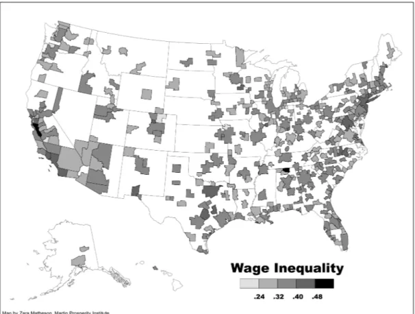
Figure 1: Wage Inequality
Figure 1 maps the regional variation of wage inequality across U.S. metros. The measure is based on the Theil Index, which is an entropy measure which will capture differences in wage between occupational groups of knowledge workers, standardized service workers, manufacturing workers, and fishing and farming workers. It is based 2010 data from the Bureau of Labor Statistics.
As the map shows, wage inequality show considerable regional variation, ranging from a low of .22 to a high more than double that,.48-.50. The metros with the highest wage inequality scores are almost all major high-tech knowledge economy regions such as: Huntsville, Alabama (a center for semiconductor and high-tech industry); San Jose (the fabled Silicon Valley); College Station-Bryan, Texas (home to Texas A&M); Boulder, Colorado (a leading center for tech startups); Durham,
North Carolina in the famed Research Triangle, and Austin (another leading high-tech center), as well as large, diverse metros such as New York, Los Angeles, greater Washington DC and San Francisco - all of which are within the top twenty metros with the most unequal wages.
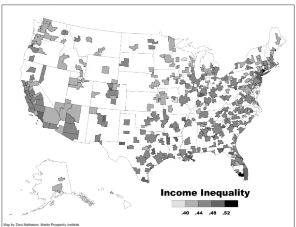
Figure 2: Income Inequality
Figure 2 maps the geography of income inequality, measured as a Gini coefficient based on data from the 2010 American Community Survey. The
geographic variation is again considerable, ranging from a low of .39 to a high of .54. But, the two maps are far from the same; in fact, they are strikingly different.
unequal metros in terms of income are smaller metros, including many resort and college towns.
Correlation Analysis
The next step in our analysis is a basic correlation analysis. We begin by looking at the bivariate relation between the regional variation in wage and income inequality across U.S. metros, before turning the wider range of independent variables included in our analysis.
Figure 3: Wage Inequality vs. Income Inequality
Figure 3 provides a scatterplot of metros on the two measures of inequality. It arrays into four basic quadrants. Metros in the upper right-hand corner face the double whammy of high income and high wage inequality. Metros in the lower right
income inequality. Metros in the upper left have high levels of income inequality alongside relatively lower levels of wage inequality. Lastly, metros in the lower left have relatively low levels of both.
Generally speaking, we find that there are metros with high levels of both wage and income inequality, as well as metros with low levels of both. There are also metros with higher levels of income inequality than what their wage inequality level would predict, as well as metros with lower levels of income equality than what their wage inequality would predict. Thus, we find a relatively weak association between the geographic variation in wage and income inequality.
We now turn to the correlation findings which compare the geographic variation in wage and inequality to variables that the literature suggests is likely to affect this geographic pattern. Table 2 summarizes the basic results of the correlation analysis.
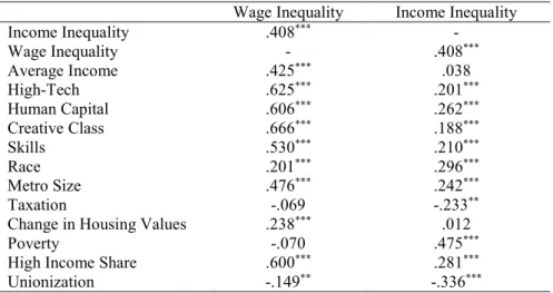
Table 2: Correlation Analysis Findings
Wage Inequality Income Inequality Income Inequality .408*** - Wage Inequality - .408*** Average Income .425*** .038 High-Tech .625*** .201*** Human Capital .606*** .262*** Creative Class .666*** .188*** Skills .530*** .210*** Race .201*** .296*** Metro Size .476*** .242*** Taxation -.069 -.233**
Change in Housing Values .238*** .012
Poverty -.070 .475***
High Income Share .600*** .281***
Unionization -.149** -.336***
***indicate significance at the 1 percent level, ** at the 5 percent level.
words, the geographies of wage and income inequality have at best a modest degree of overlap.
Beyond this, the key results of the correlation analysis point to a number of interesting geographic patterns and especially to differences between the two types of inequality
We start with the factors that might potentially relate to wage inequality. The geographic variation in wage inequality is significantly associated with factors identified in the literatures on skill-biased technical change and job polarization: human capital (.606), knowledge-based and creative occupations (.666), high-tech industry (.625), and analytical and social skills (.530). Wage inequality is also associated with high-income share (.600), average income levels (.425), and metro size (.476). Geographic variation in wage inequality is not significantly associated with poverty or taxation, and only modestly associated with race (.201), change in housing values (.238), and unionization (-.149).
We now turn to the factors that might potentially correlate with the geographic variation in income inequality. The differences in the factors associated with the two types of inequality are immediately apparent. Regional variation in income inequality is more closely related to race, poverty and indicators of the unraveling of the social compact (de-unionization and lower rates of taxation). It is most closely associated with poverty (.475) and slightly less so to race (.296). It is negatively associated with unionization (-.336), in other words inequality is higher in metros with lower levels of unionization; and it is also negatively associated with taxation (-.233), as inequality is higher in metros with lower rates of taxation. The geographic variation in income inequality is modestly associated with some of the factors identified in the literatures on skill-biased technical change and job polarization such as: human capital (.262),
the high-income share of the population (.281), metro size (.242), workforce skill (.210), high-tech industry (.201), and knowledge and creative occupations (.188). It is not significantly associated with average income or changes in housing values.
To a certain degree, the associations between income inequality and high degrees of poverty on the one hand and high degrees of affluence on the other should not be surprising. Income inequality, measured by the Gini coefficient, captures the income distribution from the bottom to the top. In other words, the share below the poverty line should be reflected by the lower part of the Lorenz curve and the share in the top income group by the higher part of the Lorenz curve (which is used to estimate the Gini). However, if incomes in general are high within a region, only a very
restricted, and small part would be equal to the lower part of the Lorenz curve (and the opposite for high income share), and not necessarily have a major impact on the overall distribution.
That said we find the actual pattern to be mixed. There are some regions that have low shares of poverty combined with relatively high levels of income inequality, e.g. Bridgeport, Naples, New York, Miami, Boston and San Francisco. There are other metros with low levels of income inequality, but with relatively high shares of poverty (e.g. Hanford, CA, Clarksville, TN-KY, and Hinesville, GA). At the same time, there are metros with high levels of income inequality and small shares of high-income individuals. Conversely, there are also metros with relatively low levels of income inequality and relatively large shares of high-income people. As table 2 shows, the correlation between income inequality and the share of high-income households is insignificant (-.070), while the correlation between income inequality and poverty is positive and significant (.475). This suggests that income inequality is
Multiple Regression Analysis
To further understand the geographic variation and regional determinants of wage and income inequality, we turn to the results of our multiple regression analysis. Our model is estimated by a basic OLS regression with inequality as the dependent
variable and a series of independent variables. We formulate our models based on the assumption that wage inequality affects income inequality, not the other way around. The first set of models are designed to test the explanatory power of different
variables related to the literatures on skill-biased technical change and job
polarization, such as skills and high-tech industry shares on the regional variation of both wage and income inequality. We then add socio-economic variables such as average income, race, changes in housing values, income taxation rates, poverty shares, high-income shares, unionization, and a control for metro size to the income inequality model, to compare their relative strength as compared to the first set of skill-biased technical change and job polarization variables. We only include socio-economic variables in the income inequality regression since the correlation analysis suggests weak associations between them and the geography of wage inequality. We do however run and report for the R2 Adjusted values for wage inequality regressions with socio-economic variables included, in order to evaluate to what extent these socio-economic variables add to the explanatory power of these regressions. All variables are in logged form, and the coefficients can be interpreted as elasticities. Since we would expect a certain degree of multicollinearity between our explanatory variables, we include a full correlation matrix in Appendix 2. We also report for the Variance Inflation Factor (VIF) values separately in relation to the analysis.
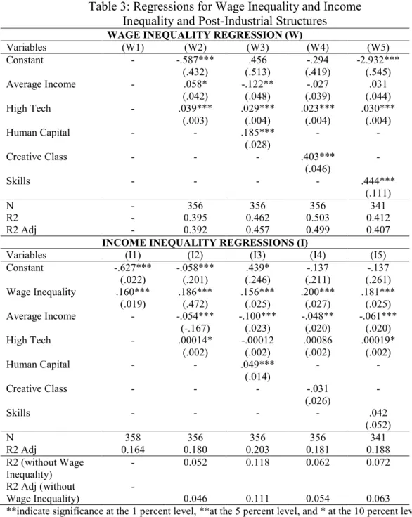
We start with the regressions for wage inequality. Table 3 summarizes the key results from the regressions where we let wage inequality as well as income inequality be explained by variables related to technical change. Due to multicollinearity issues, we run models of the three skills variables (human capital, creative class and skills) one at a time. The top of the table includes the wage inequality regressions, while the bottom illustrates the income inequality regression resultsi.
Table 3: Regressions for Wage Inequality and Income Inequality and Post-Industrial Structures WAGE INEQUALITY REGRESSION (W)
Variables (W1) (W2) (W3) (W4) (W5) Constant - -.587*** (.432) (.513) .456 (.419) -.294 -2.932*** (.545) Average Income - .058* (.042) -.122** (.048) (.039) -.027 (.044) .031 High Tech - .039*** (.003) .029*** (.004) .023*** (.004) .030*** (.004) Human Capital - - .185*** (.028) - - Creative Class - - - .403*** (.046) - Skills - - - - .444*** (.111) N - 356 356 356 341 R2 - 0.395 0.462 0.503 0.412 R2 Adj - 0.392 0.457 0.499 0.407
INCOME INEQUALITY REGRESSIONS (I)
Variables (I1) (I2) (I3) (I4) (I5) Constant -.627*** (.022) -.058*** (.201) (.246) .439* (.211) -.137 (.261) -.137 Wage Inequality .160*** (.019) .186*** (.472) .156*** (.025) .200*** (.027) .181*** (.025) Average Income - -.054*** (-.167) -.100*** (.023) -.048** (.020) -.061*** (.020) High Tech - .00014* (.002) -.00012 (.002) .00086 (.002) .00019* (.002) Human Capital - - .049*** (.014) - - Creative Class - - - -.031 (.026) - Skills - - - - .042 (.052) N 358 356 356 356 341 R2 Adj 0.164 0.180 0.203 0.181 0.188 R2 (without Wage Inequality) - 0.052 0.118 0.062 0.072 R2 Adj (without -
Equation I1 (bottom of Table 3) models the basic relationship between wage inequality and income inequality alone, based on our assumption that income inequality is a function of wage inequality. Wage inequality, while significant, explains just 16 percent of the variation in income inequality across regions.
Equation 2 adds two additional variables - average income and high-tech. In the wage inequality regression (W2), both high tech and average income are
significant and the R2 is close to 0.4. In the income inequality regression (I2) the R2 Adj. increases just slightly, compared to in W1, to .180. High-tech is weakly
significant. And surprisingly, there is a negative and significant relation between average income and income inequality. This suggests that metros with higher levels of average incomes have lower levels of income inequality. Average incomes can
increase in several ways; the poor do better; the rich do better, or everybody does better. This suggests that the gap between the bottom and the top gets closer, as the average income in regions increases. Also, if we compare the R2 generated from regression W2 and I2 (without wage inequality for comparison reasons), we find a major difference. While W2 has an R2 of 0.40, the R2 of regression I2 is only 0.05, suggesting that income inequality is significantly less explained by these variables than wage inequality. Even when wage inequality is included in the regression, the explanatory power is significantly lower than in regression W2.
Equation 3 adds human capital, measured as the percentage of adults with at least a college degree or above. In the wage inequality regression (W3), human capital, as well as high tech is significant, and the R2 Adj. increases by 0.065 to 0.457. In the income inequality regression (I3), the R2 Adj. increases slightly to .203.While human capital is positive and significant, the included variables still
explain significantly less than in the wage inequality regression. Wage inequality and average income remain significant, while high tech concentration loses its
significance in the income inequality regression (I3).
Equation 4 substitutes the variable for human capital with that of the creative class. In the wage inequality regression (W4), the creative class and high tech variables remain significant. The R2 Adj. increase even further to 0.457, suggesting that almost 50 percent of the variation in wage inequality is explained by the included variables. For the income inequality regression (I4), the pattern is still different. The R2 Adj. is even lower than in I3 (now down to 0.188), and if we compare the R2 values in W4 and I4 (when we exclude wage inequality for comparison reasons), the difference is a striking 0.441 (.503 compared to .054). The occupation variable is insignificant in I4, indicating that income inequality is not related to higher shares of creative class workers, once wage inequality and average income have been
controlled for. Equation 5 substitutes the skill variable leading to similar insignificant results, in other words, skills is significantly related to wage inequality (W5) but insignificant in relation to income inequality (I5).
Overall, our results suggest that the geographic variation in wage inequality is significantly more related to skill-biased technical change variables such as high tech and different forms of skill, while income inequality is significantly less so. We find a modest association with average income levels, human capital and to some extent high-tech industry. Creative class occupations and underlying workforce skills are insignificant once wage inequality, average income and high-tech are controlled for.
Based on this, we proceed with the next step in the regression analysis, adding the socio-economic variables and measures identified in the literatures on race,
socio-economic variables such as race, poverty, and high-income share, we also add measures of unionization, taxation, and housing values, while excluding a number of variables that were insignificant in the analysis above. We also add a control variable for metro size to examine the possible connection between metro size and inequality. We report for R2 values for wage inequality regressions below; to see to what extent they increase when socio-economic variables are added to the modelii.
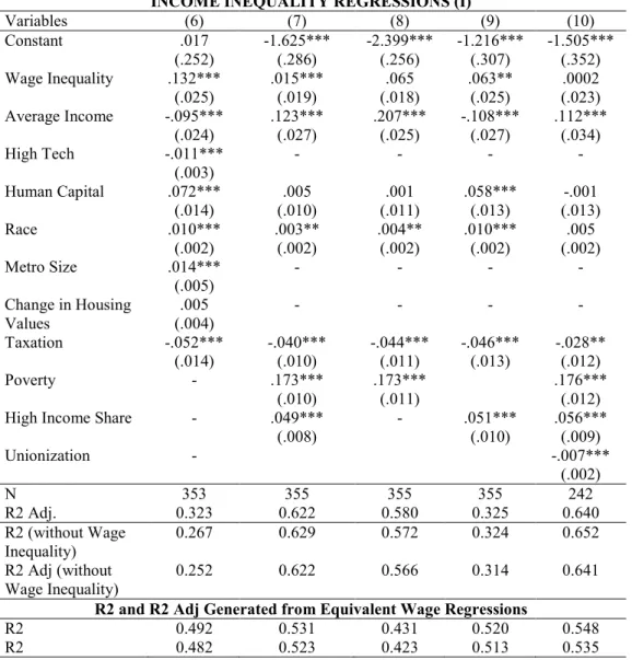
Table 4: Regressions for Wage and Income Inequality with Socio-Economic Variables Added
INCOME INEQUALITY REGRESSIONS (I)
Variables (6) (7) (8) (9) (10) Constant .017 (.252) -1.625*** (.286) -2.399*** (.256) -1.216*** (.307) -1.505*** (.352) Wage Inequality .132*** (.025) .015*** (.019) (.018) .065 .063** (.025) (.023) .0002 Average Income -.095*** (.024) .123*** (.027) .207*** (.025) -.108*** (.027) .112*** (.034) High Tech -.011*** (.003) - - - - Human Capital .072*** (.014) (.010) .005 (.011) .001 .058*** (.013) (.013) -.001 Race .010*** (.002) .003** (.002) .004** (.002) .010*** (.002) (.002) .005 Metro Size .014*** (.005) - - - - Change in Housing Values (.004) .005 - - - - Taxation -.052*** (.014) -.040*** (.010) -.044*** (.011) -.046*** (.013) -.028** (.012) Poverty - .173*** (.010) .173*** (.011) .176*** (.012) High Income Share - .049***
(.008) - .051*** (.010) .056*** (.009) Unionization - -.007*** (.002) N 353 355 355 355 242 R2 Adj. 0.323 0.622 0.580 0.325 0.640 R2 (without Wage Inequality) 0.267 0.629 0.572 0.324 0.652 R2 Adj (without Wage Inequality) 0.252 0.622 0.566 0.314 0.641
R2 and R2 Adj Generated from Equivalent Wage Regressions
R2 0.492 0.531 0.431 0.520 0.548 R2 0.482 0.523 0.423 0.513 0.535
***indicate significance at the 1 percent level, **at the 5 percent level, and * at the 10 percent level. Equation 6 indicates a strong multicollinearity for High Tech and Metro Size, with VIF values of 6.3 and 4.6. All other VIF values are below 3. There is also a strong correlation between average income and poverty, which most probably is causing the shifting sign of the average income coefficient.
Equation 6 introduces race, change in housing values, taxation, and metro size. This doubles the R2 Adj. values to .323, with positive and significant values for race and metro size, while taxation is negative and significant. This indicates that metros with higher shares of African-Americans and lower rates of taxation have higher levels of income inequality. Since we expect a strong collinearity between these variables, we also generated variance inflation factor values, which indicate that there is a relatively strong association between high-tech and metro size. We re-ran
equation 6 and included high-tech and metro size one at a time. When run individually, each variable also turned out to be insignificant. Additionally an interaction variable was created for high-tech and metro size, and it was also insignificant in this model. We thus exclude both variables in the following regressions.
In Equation 7, we add poverty and the share of high-income households. Studies by Gordon and Dew-Becker (2008), Deininger and Squire (1996) have demonstrated the consequences of poverty on levels of inequality. We note that poverty partly may be a proxy for the lower part of the Lorenz curve, while high income share is a reflection of the top of the Lorenz curve, which determines the slope of the Gini coefficient. Since this will impact the explanatory value of our model (and increase the R2 values), we add them to the model in combination, as well as one by one. Both variables as expected are significant. But interesting enough, the poverty variable is much stronger than the high-income variable. In other words, the share of the population below the poverty line explains income inequality more than the share of people with high incomes. Wage inequality, race, and taxation rates all remain significant.
In Equation 8, we only include poverty and in Equation 9, we only include high-income share, in order to be parse the relative effects of each. The regression with poverty generates an R2 adjusted of .580, substantially higher than that R2 of .325 for the regression with the high-income share variable. It is important to point out that our variable for high-income share is limited by the fact that the cut-off is $100,000 (based on the definition from the Census), and as a result, we cannot determine the exact slope of the Lorenz curve. That said, our findings still suggest income inequality is more strongly related to poverty, in other words with the bottom end of the income distribution, than to the top end of it.
In the last model, Equation 10, we include the unionized share of the labor force. Including it reduces our sample by one-third due to lack of data and this may have an effect on the estimations overall. The variable for unionization is negative and significant. In other words, unionization has a dampening effect on income inequality across metros regions. Average income remains significant in this model, but human capital does not. When we check for multicollinearity, we find relatively high VIF values between average income and human capital. To better understand this, we ran income and human capital separately. Now each variable is significant. We then created a single interaction term from both the income and human capital variables, and it remained significant. Thus, we are led to conclude human capital remains associated with income inequality and that the insignificant sign is a result of
multicollinearity in the model. We also re-ran Equation 10 with the smaller sample, but without the unionization variable. Wage inequality, human capital, and race remained insignificant. Therefore, we conclude that the insignificance of these values in Equation 10 is due to the reduced sample size rather than the inclusion of the unionization variable.
We also re-ran the equivalent regressions for wage inequality for comparison reasons. The generated R2 and R2 Adj. values can be found at bottom of Table 4. In general, adding the socio-economic variables adds little to the explanatory power of the model (compare the results to Table 3 above). The R2 Adj. values are significantly lower when only poverty is included in the model (0.423) (regression 8), and the R2 Adj. value increases by almost 0.1 (to 0.513) (regression 9), when high income shares are included instead. This suggests that the geographic variation of wage inequality is more sensitive to the top of the income distribution in comparison to the geographic variation in income inequality that is more sensitive to the bottom.
Discussion and Conclusions
Our research has examined the geographic variation in inequality across the United States. It distinguished between two distinct types of inequality: wage and income inequality. We mapped and charted the geographic variation in each across U.S. metros and presented the results of the correlation and regression analysis examining factors that the literatures on skill-biased technical change and job
polarization on the one hand and on race, class, and poverty, on the other, suggest are associated with inequality.
Perhaps the most striking finding of our analysis is found when looking at the data geographically – that is across U.S. metros –these two types of inequality turn out to be only modestly correlated with one another: Wage inequality explains 16 percent of the variation in income inequality across U.S. metropolitan regions.
The two types of inequality are also associated with very different regional clusters of variables, according to our analysis. The geographic variation in wage
biased technical change and job polarization. Wage inequality is higher in larger, more skilled regions, with higher levels of human capital, greater shares of creative class jobs, and greater concentrations of high-tech industry. The geography of wage inequality is also more driven by the top of the income distribution than by poverty. Furthermore, while the literatures on skill-biased technical change and job
polarization suggest that high- and low-skilled jobs grow in the same locations, our findings indicate that this does not necessarily imply higher levels of income inequality.
The geographic variation in income inequality is less closely associated with the factors identified by studies of job polarization and skill-biased technical change. Regional variation in income inequality is more closely associated with the geography of poverty and race (Wilson 1990) as well as de-unionization (Bluestone and
Harrison, 1988), and low tax rates. This is reinforced by the finding that income inequality tends to be negatively associated with average incomes, which suggests that more affluent metros on average are not necessarily more unequal. We also find that regional variation in income inequality is more closely associated with the geographic variation in poverty than with geographic variation in extreme affluence. We are thus led to conclude that the geographic variation in income inequality across U.S. metros is more of a consequence of the sagging taking place at the bottom of socio-economic order.
Metro size is closely related to wage inequality, but is not associated with income inequality when we control for other socio-economic variables. The geographic sorting of the population across human capital and skill groups which plays such a large role in wage inequality does not appear to play much of a role, if any, in the incidence of income inequality across metros.
For these reasons, we suggest that future research focuses on the differences and distinctions between these two kinds of inequality. While much of the current literature focuses on the effects of skill-biased technical change and job polarization, our findings remind us of the ongoing role of race and poverty as well as the
unraveling of the post-war social compact in the geography of in income inequality. Our best assessment, based on the findings of this research, is that skill-biased technical change and job polarization are a necessary but insufficient condition for explaining the geography of income inequality across U.S. metros. The enduring legacy of and geographic variation in race and poverty and the differential geographic unraveling of the post-war social compact reflected in de-unionization and low tax rates play significant roles as well. Thus, policy measures designed to address income inequality should deal with all of these factors. Most of all we hope our research and findings spur additional research on the geographic causes and consequences of inequality.
Acknowledgments:
Florida is Director of the Martin Prosperity Institute in the Rotman School of Management, University of Toronto, florida@rotman.utoronto.ca. Mellander is Research Director of the Prosperity Institute of Scandinavia, Jönköping International Business School, charlotta.mellander@ihh.hj.se. Taylor Brydges and Zara Matheson provided research assistance.
References:
Acemoglu, D. (1998). Why Do New Technologies Complement Skills? Directed Technical Change and Wage Inequality. The Quarterly Journal of Economics, 113(4), 1055 -1089. doi:10.1162/003355398555838
Acemoglu, D., & Robinson, J. (2011). Why Nations Fail: The Origins of Power, Prosperity, and Poverty. Crown.
Adams, Jr., R. (2003). Economic Growth, Inequality, and Poverty: Findings from a New Data Set. SSRN eLibrary. Retrieved from:
http://papers.ssrn.com/sol3/papers.cfm?abstract_id=1357182
Atkinson, A., Piketty, T., & Saez, E. (2011). Top Incomes in the Long Run of History. Journal of Economic Literature, 41(9), 3-71. doi: Urban inequality: evidence from four cities
Autor, D. H., Katz, L. F., & Kearney, M. S. (2006). The Polarization of the U.S. Labor Market. National Bureau of Economic Research Working Paper Series, No. 11986. Retrieved from http://www.nber.org/papers/w11986
Autor, D. H., Katz, L. F., & Krueger, A. B. (1998). Computing Inequality: Have Computers Changed the Labor Market?. Quarterly Journal of Economics, 113(4), 1169-1213. doi:10.1162/003355398555874
Autor, D. H., Levy, F., & Murnane, R. J. (2003). The Skill Content of Recent Technological Change: An Empirical Exploration. Quarterly Journal of Economics, 118(4), 1279-1333. doi:10.1162/003355303322552801
Ballas, D. (2004). Simulating Trends in Poverty and Income Inequality on the Basis of 1991 and 2001 Census Data: A Tale of Two Cities. Area, 36(2), 146-163.
Bartels, L. M. (2010). Unequal Democracy: The Political Economy of the New Gilded Age. Princeton University Press.
Bartik, T. J. (1992) “The Effects of State and Local Taxes on Economic
Development: A Review of Recent Research”, Economic Development Quarterly, 6, pp.102-111.
Bartik, T. J. (2002) Evaluating the Impacts of Local Economic Development Policies on Local Economic Outcomes: What Has Been Done and What is Doable?,
(November 2002). Upjohn Institute Staff Working Paper No. 03-89. Available at SSRN: http://ssrn.com/abstract=369303
Baum-Snow, N., & Pavan, R. (2011). Inequality and City Size (pp. 1-33). The National Bureau of Economic Research. Retrieved from
http://www.econ.brown.edu/fac/Nathaniel_Baum-Snow/ineq_citysize.pdf Berry, C. R., & Glaeser, E. L. (2005). The Divergence of Human Capital Levels Across Cities. Papers in Regional Science, 84(3), 407-444. doi:10.1111/j.1435-5957.2005.00047.x
Betz, D. M. (1974). A Comparative Study of Income Inequality in Cities. The Pacific Sociological Review, 17(4), 435-456.
Bishop, B. (2008). The Big Sort: Why the Clustering of Like-Minded America Is Tearing Us Apart (None.). Houghton Mifflin Harcourt.
Bluestone, B., & Harrison, B. (1982). The Deindustrialization of America: Plant Closing, Community Abandonment, and the Dismantling of Basic Industry, New York: Basic Books.
Bluestone, B., & Harrison, B. (1986). The Great American Job Machine: The Proliferation of Low Wage Employment In the US Economy, Study prepared for the Joint Economic Committee, available at:
xtSearch_SearchValue_0=ED281027&ERICExtSearch_SearchType_0=no&accno=E D281027
Bluestone, B., & Harrison, B. (1988). The Growth of Low-Wage Employment: 1963-86, The American Economic Review, 78(2), 124-128.
Borjas, G. J. (1995). The Internationalization of the U.S. Labor Market and the Wage Structure. Economic Policy Review, 1(1): 3-9. Retrieved from
http://papers.ssrn.com/sol3/papers.cfm?abstract_id=1029649
Borjas, G. J., & Ramey, V. A. (1995). Foreign Competition, Market Power, and Wage Inequality. The Quarterly Journal of Economics, 110(4), 1075 -1110.
doi:10.2307/2946649
Braun, D. (1988). Multiple Measurements of U.S. Income Inequality. The Review of Economics and Statistics, 70(3), 398-405. doi:10.2307/1926777
Burgers, J., & Musterd, S. (2002). Understanding Urban Inequality: A Model Based on Existing Theories and an Empirical Illustration. International Journal of Urban and Regional Research, 26(2), 403-413. doi:10.1111/1468-2427.00387
Card, D., & DiNardo, J. E. (2002). Skill Biased Technological Change and Rising Wage Inequality: Some Problems and Puzzles. National Bureau of Economic Research Working Paper Series, No. 8769. Retrieved from:
http://www.nber.org/papers/w8769
Colenutt, B. (1970). Poverty and Inequality in American Cities. Antipode, 2(2), 55-60. doi:10.1111/j.1467-8330.1970.tb00481.x
Collins, R. W., & Morris, R. A. (1988). Racial Inequality in American Cities: An Interdisciplinary Critique. National Black Law Journal, 11, 177.
DeVol, R., Wong, P., Catapano,J., & Robitshek,G. (2001) America’s High-Tech Economy; Growth, Development, and Risks for Metropolitan Areas, Milken Institute.
Donegan, M., & Lowe, N. (2008). Inequality in the Creative City: Is There Still a Place for “OldFashioned” Institutions? Economic Development Quarterly, 22(1), 46 -62. doi:10.1177/0891242407310722
Fan, C. C., & Casetti, E. (1994). The spatial and temporal dynamics of US regional income inequality, 1950–1989. The Annals of Regional Science, 28(2), 177-196. doi:10.1007/BF01581768
Florida, R. (2002a). The Rise Of The Creative Class: And How It’s Transforming Work, Leisure, Community And Everyday Life (1st ed.). Basic Books.
Florida, R. (2002b). The Economic Geography of Talent. Annals of the Association of American Geographers, 92(4), 743-755. doi:10.1111/1467-8306.00314
Florida, R., Mellander, C., & Stolarick, K. (2008). Inside the black box of regional development—human capital, the creative class and tolerance. Journal of Economic Geography, 8(5), 615 -649. doi:10.1093/jeg/lbn023
Florida, R., Mellander, C., Stolarick, K., & Ross, A. (2011). Cities, skills and wages. Journal of Economic Geography. doi:10.1093/jeg/lbr017
Gabbidon, S. L., & Greene, H. T. (2005). Race, crime, and justice: a reader. Routledge.
Gavin, S. (2007). Global cities of the South: Emerging perspectives on growth and inequality. Cities, 24(1), 1-15. doi:10.1016/j.cities.2006.10.002
Glaeser, E. L., Resseger, M., & Tobio, K. (2009). Inequality in Cities. Journal of Regional Science, 49(4), 617-646. doi:10.1111/j.1467-9787.2009.00627.x
Goldin, C. D., & Katz, L. F. (2008). The race between education and technology. Harvard University Press.
Goldsmith, W. W., Blakely, E. J., & Clinton, B. (2010). Separate Societies: Poverty and Inequality in U.S. Cities. Temple University Press.
Goos, M., Manning, A. (2007) "Lousy and Lovely Jobs: The Rising Polarization of Work in Britain.", Review of Economics and Statistics, 89(1): 118-33.
Goos, M, Manning, A., Salomons, A. (2009), Job Polarization in Europe, The American Economic Review, Vol 99:2, pp. 58-63
Gordon, R. J., & Dew-Becker, I. (2008). Controversies about the Rise of American Inequality: A Survey. National Bureau of Economic Research Working Paper Series, No. 13982. Retrieved from http://www.nber.org/papers/w13982
Gould, E. D. (2007). Cities, Workers, and Wages: A Structural Analysis of the Urban Wage Premium. Review of Economic Studies, 74(2), 477-506. doi:10.1111/j.1467-937X.2007.00428.x
Gould, Eric D., & Paserman, M. D. (2003). Waiting for Mr. Right: Rising Inequality and Declining Marriage Rates. Journal of Urban Economics, 53(2), 257-281.
doi:10.1016/S0094-1190(02)00518-1
Hunter, B. H. (2003). Trends in Neighbourhood Inequality of Australian, Canadian, and United States of America CitiesSsince the 1970s. Australian Economic History Review, 43(1), 22-44. doi:10.1111/0004-8992.00039
Hunter, B., & Gregory, R. G. (1996). An Exploration of The Relationship Between Changing Inequality Of Individual, Household And Regional Inequality In Australian Cities. Urban Policy and Research, 14(3), 171-182. doi:10.1080/08111149608551594
Kuznets, S. (1955). Economic Growth and Income Inequality. The American Economic Review, 45(1), 1-28.
Lerman, R. I., & Yitzhaki, S. (1985). Income Inequality Effects by Income Source: A New Approach and Applications to the United States. The Review of Economics and Statistics, 67(1), 151-156. doi:10.2307/1928447
Manning, A. (2004) “We Can Work It Out: The Impact of Technological Change on the Demand for Low-Skill Workers”, Scottish Journal of Political Economy, Vol 51:5, pp. 581-608
Martin, R. (1997). Can High-Inequality Developing Countries Escape Absolute Poverty? Economics Letters, 56(1), 51-57. doi:10.1016/S0165-1765(97)00117-1 McCall, L. (2000). Explaining Levels of Within-Group Wage Inequality in U.S. Labor Markets. Demography, 37(4), 415-430. doi:10.1353/dem.2000.0008 McCall, L. (2001). Sources of Racial Wage Inequality in Metropolitan Labor Markets: Racial, Ethnic, and Gender Differences. American Sociological Review, 66(4), 520-541. doi:10.2307/3088921
Mincer, J. (1996). Economic Development, Growth of Human capital, and the Dynamics of the Wage Structure. Journal of Economic Growth, 1(1), 29-48. doi:10.1007/BF00163341
Moretti, E. (2008). Real Wage Inequality. National Bureau of Economic Research Working Paper Series, No. 14370. Retrieved from:
http://www.nber.org/papers/w14370
Murphy, K., Riddell, C., and Romer, P. (1998). Wages, Skill, and Technology in the United States and Canada, in General Purpose Technologies and Economic Growth,
Nord, S. (1980). An Empirical Analysis of Income Inequality and City Size. Southern Economic Journal, 46(3), 863-872. doi:10.2307/1057154
Obama, Barack (2011). Remarks by the President on the Economy in Osawatomie, Kansas, December 6, 2011, Available at: http://www.whitehouse.gov/the-press-office/2011/12/06/remarks-president-economy-osawatomie-kansas
O’Connor, A., Tilly, C., & Bobo, L. (2001). Urban Inequality: Evidence From Four Cities. Russell Sage Foundation.
Sampson, R. J. (1995) “The Community”, in Crime and Public Policy, eds. Wilson, J. Q., Petersilia, J. San Francisco: Inst. Contemporary Studies Press, pp. 193-216 Semyonov, M., Haberfeld, Y., Cohen, Y., & Lewin-Epstein, N. (2000). Racial Composition and Occupational Segregation and Inequality across American Cities. Social Science Research, 29(2), 175-187. doi:10.1006/ssre.1999.0662
Sharkey, P. (2013) Stuck in Place: Urban Neighborhoods and the End of Progress Toward Racial Equality, Chicago: University of Chicago Press.
Shihadeh, E. S., & Steffensmeier, D. J. (1994). Economic Inequality, Family Disruption, and Urban Black Violence: Cities as Units of Stratification and Social Control. Social Forces, 73(2), 729 -751. doi:10.1093/sf/73.2.729
Smith, S. S. (2000). Mobilizing Social Resources: Race, Ethnic, and Gender Differences in Social Capital and Persisting Wage Inequalities. The Sociological Quarterly, 41(4), 509-537. doi:10.1111/j.1533-8525.2000.tb00071.x
Steelman, A., & Weinberg, J. A. (2005). What’s Driving Wage Inequality? (pp. 1-17). Federal Reserve Bank of Richmond. Retrieved from:
Stephens, C. (1996). Healthy Cities or Unhealthy Islands? The Health and Social Implications of Urban Inequality. Environment and Urbanization, 8(2), 9 -30. doi:10.1177/095624789600800211
Stiglitz, J. E. (1969). Distribution of Income and Wealth Among Individuals, Econometrica, 37(3), 382-397.
Stiglitz, J. (May 2011) “Of the 1%, by the 1%, for the 1%,” Vanity Fair. Retrieved from:
http://www.vanityfair.com/society/features/2011/05/top-one-percent-201105?currentPage=all&wpisrc=nl_wonk
Tanzi, V., & Chu, K.Y. (1998). Income Distribution and High-Quality Growth. MIT Press.
Timberlake, J. M., & Iceland, J. (2007). Change in Racial and Ethnic Residential Inequality in American Cities, 1970–2000. City & Community, 6(4), 335-365. doi:10.1111/j.1540-6040.2007.00231.x
Wheeler, C. (2005a). Evidence on Wage Inequality, Worker Education and
Technology (pp. 375-395). Federal Reserve Bank of St. Louis Review. Retrieved from http://65.89.18.138/publications/review/05/05/Wheeler.pdf
Wheeler, C. H. (2004). Wage Inequality and Urban Density. Journal of Economic Geography, 4(4), 421 -437. doi:10.1093/jnlecg/lbh033
Wheeler, C. H. (2005b). Cities, Skills, and Inequality. Growth and Change, 36(3), 329-353. doi:10.1111/j.1468-2257.2005.00280.x
White, M. J. (1981). Optimal Inequality in Systems of Cities or Regions. Journal of Regional Science, 21(3), 375-387. doi:10.1111/j.1467-9787.1981.tb00707.x
Wilson, W. J. (1990). The Truly Disadvantaged: The Inner City, the Underclass, and Public Policy (1st ed.). University Of Chicago Press.
Appendix 1: The skills variable
We build on the work by Florida et al. (2011) to calculate the skills variable. We start by measures the skill value for each occupation. It is based on the O*NET database which was developed for the U.S. Department of Labor, and contains detailed analysis conducted by occupational specialists, occupational analysts, and job incumbents. They quantify how much of a certain “skill” is required for each of 728 occupations, resulting in 87 identified skill variables. We used exploratory cluster analysis to categorize these 87 skill variables in three distinct groupings: (1) analytical skills, (2) social intelligence skills and (3) physical skills.
Once the groups were identified through cluster analysis, we created the skill scores. The 87 “skill” and “ability” variables, as defined by O*NET, measure various dimensions of occupational requirements. Each variable has two components -- importance (on a 1-5 scale) and level (on a 0-7 scale). We multiplied the scales
together to obtain a single measure for each variable, and then took the percentile rank across all occupations. To generate the skill scores we employed in the analysis, we took the occupational skill percentile and weighted it by employment share in each occupation for each region. The score for a region tells us the average skill percentile across all occupations. The data is a combination of the O*NET data and BLS data for occupations.
In this analysis, we include a combination of analytical and social skills, equally weighted. Analytical skills mainly consist of a numerical facility, and general cognitive functioning, involving skills such as developing and using rules and methods to solve problems. Social skills have a personal element and are related to skills such as understanding, collaborating with, and managing other people. The
of 0.694. Because of this, we turn the social and analytical variable into one single variable through a principle component analysis, where the generated social analytical measure variable correlate with the analytical score variable with 0.903 and the social score variable with 0.934.
Appendix 2: Correlation Matrix
Average
Income High-Tech Human Capital Creative Class Skills Race Metro Size Taxation
Change in Housing Values Poverty High Income Share Unionization Average Income 1 .602** .737** .548** .510** -.004 .417** .098 .526** -.725** .783** .132* High-Tech .602** 1 .662** .672** .648** .145** .845** -.051 .398** -.360** .732** .105 Human Capital .737** .662** 1 .749** .500** -.062 .403** .012 .419** -.353** .648** .001 Creative Class .548** .672** .749** 1 .631** .100 .457** .014 .282** -.184** .564** .161* Skills .510** .648** .500** .631** 1 .198** .538** -.042 .095 -.271** .564** .002 Race -.004 .145** -.062 .100 .198** 1 .276** -.127* -.230** .176** .100 -.193** Metro Size .417** .845** .403** .457** .538** .276** 1 -.071 .338** -.224** .641** .106 Taxation .098 -.051 .012 .014 -.042 -.127* -.071 1 .156** -.136** .010 .299**
Change in Housing Values .526** .398** .419** .282** .095 -.230** .338** .156** 1 -.430** .607** .199**
Poverty -.725** -.360** -.353** -.184** -.271** .176** -.224** -.136** -.430** 1 -.487** -.191**
High Income Share .783** .732** .648** .564** .564** .100 .641** .010 .607** -.487** 1 .082
Unionization .132* .105 .001 .161* .002 -.193** .106 .299** .199** -.191** .082 1
End Notes
i We also tested for two alternative measures for industry mix – manufacturing share and the share of education and health care sector
employment (this variable can also serve as a proxy for governmental share of employment). The results were similar to the high tech variable. Both of these variables were more closely related to wage inequality than income inequality. These industry-mix variables however generated severe multicollinearity problems when integrated in the current models. Also, when we substituted the high tech variable for the manufacturing and education and health care variables, these new variables became insignificant once skills were controlled for.
ii The wage inequality regressions are slightly different than the income inequality regressions, since we do not assume wage inequality to be a