The allocation of transport infrastructure in Swedish municipalities : welfare maximization, political economy or both?

The allocation of transport infrastructure in Swedish

municipalities: Welfare maximization, political economy or

both?

Johanna Jussila Hammes and Jan-Eric Nilsson – VTI CTS Working Paper 2015:4

Abstract

The choice of transport infrastructure projects to include in the National Transport Infrastructure Plans in Sweden is often said to be motivated by the weighing of cost against social benefits. Examining the projects that are included in the Plans, it is clear, however, that not all projects have positive net present values, and are therefore more costly to build than the benefits they create. This paper studies alternative models that might explain the choice of projects. Two political economy models, the district demand and the swing voter with lobbying, are tested, and a model that accounts for the spatial distribution of the projects, as well as the possibility that priorities are based on welfare concerns, is estimated. No support is found for the political economy models. What explains investment volume is the existence of CBA results for a project, which may indicate that welfare benefits have an impact, as do the spatial spillovers from a project’s benefits and lobbying, especially by the municipalities concerned.

Keywords: Distributive politics; Fiscal federalism; Lobbying; Party competition; Political

economy; Transport infrastructure; Spatial analysis; Sweden

JEL Codes: D6; D72; D78; R42

Centre for Transport Studies SE-100 44 Stockholm

Sweden

The allocation of transport infrastructure in Swedish municipalities: Welfare maximization, political economy or both?

Authors: Johanna Jussila Hammes and Jan-Eric Nilsson

Address: Swedish National Road and Transport Research Institute, VTI and Centre for Transport Studies Stockholm, CTS; Box 55685; SE-102 15 Stockholm. E-mail:

johanna.jussila.hammes@vti.se; jan-eric.nilsson@vti.se. Tel: 00-46-8-555 77 035

Acknowledgements: Paper presented at the National Transport Research Conference in Gothenburg, Sweden, 22 September 2013, a VTI seminar in December 2013 and the Nordic Meeting in Transport Economics in Oslo, 26 November 2014. The work has been financed by the Centre for Transport Studies Stockholm.

Abstract: The choice of transport infrastructure projects to include in the National Transport Infrastructure Plans in Sweden is often said to be motivated by the weighing of cost against social benefits. Examining the projects that are included in the Plans, it is clear, however, that not all projects have positive net present values, and are therefore more costly to build than the benefits they create. This paper studies alternative models that might explain the choice of projects. Two political economy models, the district demand and the swing voter with lobbying, are tested, and a model that accounts for the spatial distribution of the projects, as well as the possibility that priorities are based on welfare concerns, is estimated. No support is found for the political economy models. What explains investment volume is the existence of CBA results for a project, which may indicate that welfare benefits have an impact, as do the spatial

Keywords: Distributive politics; Fiscal federalism; Lobbying; Party competition; Political economy; Transport infrastructure; Spatial analysis; Sweden

1 Introduction

A growing literature views economic-policy decisions as resulting from the maximization by incumbent politicians of objective functions that are not necessarily correlated with social welfare. In addition to resource constraints, the politico-institutional structure and the wish of politicians to be re-elected in order to implement their respective policy agendas are suggested as candidates for understanding the priorities in actual decision-making. Using information about investment in transport infrastructure in France, Cadot et al., (2006) is one example of this literature. Other political economy studies of transport infrastructure investments include Fridstrøm and Elvik (1997), Helland and Sørensen (2009), both of whom study the allocation of road-project funding in Norway, and Knight (2004), who examines the allocation of transport projects in the US.

A related literature studies decision-makers’ prioritization of infrastructure projects from a welfare perspective. The point of departure in Nilsson (1991) was the government’s formal directive to take the maximization of social welfare into account when establishing an

investment program for national road infrastructure in Sweden.1 _{No relationship between social}

welfare and actual priorities could be established, and no other rationale for priorities was found. Policies in Sweden have subsequently been adjusted, primarily by shifting the ultimate control over project prioritization from the sector agency to the government itself. Later

1 _{The means for meeting this target was to rank projects based on the results of a Cost Benefit Analysis (CBA),}

summarized in terms of Net Present Value (NPV=B-C), B and C representing the present value of benefits and costs over the expected lifetime of a project. Because of budget constraints, projects with a higher NPV ratio (=NPV/C) were to be prioritized over less beneficial projects.

research still indicates that the results of a CBA in Sweden at best provide a partial explanation of project prioritization; cf. Eliasson and Lundberg (2011) and Jussila Hammes (2013). Similar observations have been made in Norway (Odeck (1996), Fridstrøm and Elvik (1997), Welde et al. (2013)), Estonia (Kõrbe Kaare & Koppel, 2012), Mexico (Ramírez Soberanis, 2010), France

(Quinet, 2010) and the United Kingdom (Mackie, 2010).

A third strand of literature studies the strategic interaction that emanates from “benefit spill-overs” (Brueckner, 2003) between tiers of government The main thrust of this literature, some of which is briefly surveyed in the next section, has been in estimating the size of the spillover effects across municipalities and regions.

It is difficult to provide a single comprehensive explanation for what drives this type of

prioritization, at least in an international perspective. This paper combines the three strands of literature: political economy modelling, assessment of the impact of welfare considerations on project choice, and implications of spillover effects from investment in one region on its neighbors, in order to shed some light on what, specifically, drives policy decisions as

manifested in three national transport infrastructure investment programs in Sweden. The first program was established by a center-left government, and the other two by a center-right government; this also provides an opportunity to test whether or not infrastructure projects are void of political preferences per se.

The paper is organized as follows: The next section briefly summarizes some relevant literature and provides a background, whereafter the theoretical background and the hypotheses are

presented. Section 4 describes the data, section 5 contains the regression results and section 6 concludes the paper with a discussion.

2 Background

Political economics offers several explanations for the preferences that guide the provision of public services. In this paper, we examine three of these. The district demand model starts by noting that spending on public goods, here transport infrastructure, provides benefits that primarily are geographically concentrated, while costs are paid by taxpayers at large. This separation between the benefits and costs of projects may create an incentive for political parties to increase spending in electoral districts or municipalities that predominately vote for them. Since each district pays only a small share of the associated costs, but enjoys most of the benefits, new infrastructure may be seen as a prize won by the political majority for their constituency. In addition, and in order to avoid overspending, parties have reason to restrain spending in other districts (Knight, 2004).

The swing-voter theory provides a second explanation. Rather than focusing on the stock of loyal voters, this assumes that two competing (blocks of) parties maximize their national vote by offering different levels of spending to election districts depending on the propensity of the voters in each district to “swing” their vote (Helland & Sørensen, 2009). Districts that ex ante are believed to be affected in their choice on polling day by projects “given by benevolent decision-makers” are therefore rewarded with new infrastructure. A third candidate explanation is that local interest groups seek to convince parliamentary decision makers to allocate infrastructure funds to their home district. This is relevant if a district’s electorate is not

very volatile, that is, given that the above-described electoral concerns are not very strong (Cadot et al., 2006).

While voting by well-informed citizens reveals the voters’ preferences, the three political economy models do not yield a definite weighing between considerations of social welfare, on the one hand, and electoral considerations and lobbying on the other. The weighing of social welfare against lobbying has been modeled by Grossman and Helpman (1994; 2001). Their model does not include voting, however.2

Although most benefits from an infrastructure project accrue to those living closest to it, it is also feasible that residents in neighboring municipalities or electoral districts may benefit (Brueckner, 2003). An early paper addressing the spillover effects from infrastructure investments is by Case, et al. (1993), who formalize and test the notion that (US) state

expenditure depends on the spending of neighboring states. They show that an increase in the expenditure of a state’s neighbors increases its own expenditure. Related to this, Ihara (2008) shows how geography can influence the provision of local public goods. Of special interest are falling transport costs, which can change the provision status of local public goods from under-provision to over-under-provision. Gutiérrez, et al., (2010) use accessibility indicators to measure and monetize the spatial spillovers of transport infrastructure investments. Their analysis separates direct investments (what is actually invested in a region) from real investments (the benefits

2 _{Grossman and Helpman (1996) consider voting, but exclude the social welfare aspect by concentrating on}

informed and uninformed voters and the incentives of politicians to receive campaign contributions in order to influence the latter voters.

accruing to a region from all investments). Dembour and Wauthy (2009) study the impact that infrastructure spillovers have on tax competition between regions. Rather than looking at the transport infrastructure, Guriev, et al. (2010) examine the spatial distribution of interest groups within a federation and show how this influences firms’ performance.

In this paper we argue that accounting for spillover effects may provide an additional

explanation for any discrepancy between the ‘socially optimal’ and observed provision of public goods. This is based on the numerous examples of large infrastructure projects that benefit the residents in a whole region, not only those of the municipality where the project is built.

Using spending on national-level transport infrastructure projects and information on the

projects and the municipalities where they are built, this paper examines how these models fare in explaining observed priorities. We test the basic model, which explains investment spending in a municipality with social welfare, against two alternative political economic models, i.e. the district demand model, and the swing-voter model including the impact of lobbying. We also test all models including a spatial aspect to account for the spillover effects.

Helland and Sørensen (2009) make a comprehensive survey of the results of previous tests of both district demand and swing-voter models. Therefore, for the purposes of this paper, it is necessary only to highlight the results of a few previous transport or Sweden-related analyses. Knight (2004) finds empirical support for his hypothesis about common pool incentives from an analysis of 1998 US Congressional votes on transportation project funding. Thus, the probability of a political representative supporting funding for projects is increasing in a legislator’s own-district spending and decreasing in the tax burden associated with aggregate spending.

Helland and Sørensen (2009) find no support for the district demand model in their analysis of road investments in Norway for the period 1973 to 1997, but the swing voter model rationalized observed priorities. They also note that high levels of party identification – a measure of voter’s resistance to being ‘bribed’ by central allocations of funds – reduce investments. A panel of French regions, used by Cadot et al. (2006) to examine the determinants of transport

infrastructure investments over the period 1985-1992, also indicates that electoral concerns and influence activities (lobbying) were significant in explaining the cross-regional allocation of investments. Johansson (2003) tests the swing voter model by using another type of good for which incentives are similar to infrastructure investment, namely intergovernmental grants in Sweden between 1981 and 1995. She also finds support for the swing voter model.

3 Hypotheses

In this section we reproduce, with some modifications, the models for district demand (Helland & Sørensen, 2009) and swing voters with lobbying (Cadot et al. 2006; Helland and Sørensen, 2009). The models generate six hypotheses.

3.1 District demand

A utility function over private and public consumption is defined for citizen 𝑖 in municipality 𝑗 ∈ 𝐽. Citizens enjoy equal amounts of pre-tax income 𝑦𝑖𝑗 = 𝑦𝑗, private consumption 𝑐𝑖𝑗 = 𝑐𝑗, and

public service consumption, 𝑔𝑖𝑗+ 𝜌 ∑𝑘≠𝑗𝑔𝑖𝑘 = 𝑠𝑗. The second term in this expression is due to

the fact that municipality j has 𝑘 = {1, … , 𝑞} neighbors, and if 𝜌 > 0, the neighbors’ level of public service provision also affects the consumption of individuals residing in municipality 𝑗. The aggregate supply of public services sums over municipalities so that ∑_𝑗∈𝐽𝑔_𝑗 = 𝑔. For

tractability, all municipalities are assumed to have an equal number of neighbors. The utility function for citizen 𝑖 ∈ (𝑛1, 𝑛2, … , 𝑛𝐼) in municipality 𝑗 = {1, 2, … , 𝐽} is then:

(1) 𝑈𝑖𝑗 = 𝑐𝑖𝑗+ 𝐻(𝑠𝑗).

Utility is linear in private income, and 𝐻′(𝑠_𝑗) > 0 with 𝐻′′_(𝑠

𝑗) < 0. Let 0 ≤ 𝜏 ≤ 1 be the

national income tax rate. The private budget constraint is:

(2) 𝑐𝑗 = (1 − 𝜏)𝑦𝑗.

Substituting (2) into (1) gives the indirect utility function for a representative citizen in municipality j

(3) 𝑉𝑗(𝜏, 𝑦𝑗, 𝑠𝑗) = (1 − 𝜏)𝑦𝑗+ 𝐻(𝑠𝑗)

The national income is 𝑦 = ∑_𝑗∈𝐽𝑦_𝑗, and since the government is assumed to balance the budget, the government’s budget constraint can be written as:

(4) _{𝜏𝑦 = ∑ 𝑔}

𝑗 𝑗∈𝐽

= 𝑔.

Substituting (4) into (3) yields

(5)

𝑣_𝑗(𝑦_𝑗, 𝑠_𝑗) = (1 −∑𝑗∈𝐽𝑔𝑗

𝑦 ) 𝑦𝑗+ 𝐻(𝑠𝑗). The socially optimal supply of public services is established by solving max

𝑔𝑗 ∑𝑗∈𝐽𝑣𝑗. Assuming

that 𝐻′(𝑠_𝑗) = 𝐻′(𝑠_𝑘) ∀𝑗, 𝑘, 𝑗 ≠ 𝑘 the FOC from (5) is

Because of the concavity of 𝐻(𝑠𝑗), higher marginal benefits imply that the optimal supply of

public services (𝑠𝑗) is lower; cf. Figure 1. 𝐻′(𝑔𝑗∗) = 1 represents the social optimum without

spillovers, and the social optimum with spillovers exceeds this level. The spillover from public service consumption in municipality 𝑗 to the neighboring municipalities 𝑘 thus generates a socially optimal provision of public services at a higher level than when only municipality 𝑗 benefits from the service.

Figure 1. Three optima. The socially optimal level of infrastructure provision in the absence of spill-over effects is given by the point where 𝑯′(𝒈_𝒋∗) = 𝟏, yielding infrastructure investment at 𝒈_𝒋∗. With spill-over effects the social optimum moves to 𝑯′(𝒔_𝒋∗) = (𝟏 + 𝒈𝝆)−𝟏, with

𝐻′(𝑠𝑗) 𝑔𝑗 𝑔_𝑗∗ 𝑠_𝑗∗ 𝑠𝑗 𝐻′(𝑠𝑗) 𝐻′(𝑔𝑗∗) = 1 𝐻′_(𝑠 𝑗′) = 1 1 + 𝑔𝜌 𝐻′(𝑠𝑗) = 𝑦𝑗 𝑦

infrastructure investment 𝒔𝒋∗. The politically optimal provision according to the district demand

model is 𝑯′(𝒔𝒋) = 𝒚𝒋/𝒚, which yields infrastructure investment 𝒔𝒋.

Suppose municipality 𝑗’s representative in the national parliament plays a one-shot,

simultaneous move game with the representatives of the 𝐽 − 1 other municipalities. The Nash equilibrium in pure strategies is found by maximizing municipality 𝑗’s indirect utility function with respect to 𝑔𝑗, taking the choice of the 𝐽 − 1 other municipalities as given. The equilibrium

outcome is:

(7) _𝐻′_(𝑠

𝑗) =

𝑦𝑗

𝑦.

Since 𝑦𝑗/𝑦 < 1, the Nash equilibrium indicates that the left-hand side is sub-optimal; 𝐻′(𝑠𝑗) <

𝐻′(𝑔_𝑗∗). As a result, the supply of the public good exceeds the optimal level (see Figure 1). This holds even with spillovers as long as municipality 𝑗’s share of national income is low enough, i.e. as long as 𝑦 > 𝑦_𝑗(1 + 𝑞𝜌). A representative therefore endeavors to persuade the central

government to allocate more funds to her municipality/electoral district than is socially optimal.

Using Equation (4) to express (7) in terms of tax revenue yields 𝐻′(𝑠𝑗) = 𝜏𝑦𝑗/𝑔, where 𝜏 and 𝑔

are given. This yields a testable hypothesis:

Hypothesis 1: National funding of transport infrastructure in a municipality decreases as the tax share of the district increases.

The district demand model is the “conventional explanation” for the observation that elected politicians bias the allocation of public services, in this case infrastructure projects, in order to favor their own election districts to win votes. But the larger the share of this investment that

the municipality has to pay for itself, i.e. the closer 𝑦𝑗 is to 𝑦, the closer to the narrowly defined

optimum the representative wants to be. And if 𝑦𝑗 = 𝑦 the representative would strive for

𝐻′_(𝑠

𝑗) = 1 and there would be under investment from the perspective of spillover effects. 3.2 Swing voters with lobbying

The originators of the swing voter model are Lindbeck and Weibull (1987) and Dixit and Lodregan (1996). We complement this with lobbying á la Cadot et al. (2006). The basic model implies that voters not only have preferences over (public and private) consumption, but also over ideological positions. Individuals who attach great importance to a party’s ideological stand have an enduring tendency to support that particular political party, and are therefore hard to swing, while voters who primarily value political parties for the consumption opportunities they provide are more attractive political prey. A major shift in the allocation of public expenditure per capita is needed to swing the ideologically oriented voters towards the other block (Helland & Sørensen, 2009, pp. 9, 11).

More specifically, two exogenously given parties compete for seats in a national assembly. Citizens cast their votes in 𝐽 separate election districts, each with a fixed number of seats proportional to the population in each district. Let 𝑔_𝑗𝑃, 𝑃 = {𝐴, 𝐵} be the amount of public good in district 𝑗 announced before an election by party 𝑃 = {𝐴, 𝐵}.

Candidates maximize an expected rent based on the number of mandates obtained and a rent from being in office, itself made up of two components. The one is an exogenous term 𝛿

reflecting utility from ideology.3 _𝛿𝑃 _{is assumed to be fixed for the duration of the electoral}

campaign, and is without loss of generality assumed to be 𝛿𝐴 = −1

2 and 𝛿 𝐵₌ 1

2. The other

component 𝑅(𝑔_𝑗𝑃) is endogenous, and is interpreted as a post-political life reward (position on a board or so) offered by a lobby interested in 𝑔_𝑗𝑃 and conditioned on the policy promised and implemented. Thus, 𝑅(𝑔_𝑗𝑃) can only be earned if party 𝑃’s candidate wins the election. The candidate’s utility is therefore summarized by (8).

(8)

𝑣𝑃 = {|𝛿𝑃| + 𝑅(𝑔𝑗𝑃)

0

if the candidate from party 𝑃 is elected otherwise

Let 𝑚𝑃(𝑔_𝑗𝐴, 𝑔_𝑗𝐵) be the share of mandates going to party 𝑃 given platforms 𝑔𝑗𝐴 and 𝑔𝑗𝐵. A party’s

problem is thus

max

𝑔𝑗 𝑚𝑗 𝑃_(𝑔

𝑗𝐴, 𝑔𝑗𝐵)[|𝛿𝑃| + 𝑅(𝑔𝑗𝑃)]

Voter 𝑖 in the electoral district 𝑗 gets utility both from consumption and from ideology:

𝑈_𝑖𝑗𝑃 = 𝜅𝑗[𝑐𝑗𝑃+ 𝐻(𝑠𝑗𝑃)] −

1

2(𝛿𝑖𝑗− 𝛿

𝑃₎2_{, 𝑃 = {𝐴, 𝐵}.}

𝜅_𝑗 measures the weight put on (public and private) consumption relative to ideology and 𝛿𝑖𝑗

denotes voter 𝑖’s ideal position.

The individual’s and the government’s budget constraints are similar to those defined above:

(9) 𝑐_𝑗𝑃 = (1 − 𝜏𝑃)𝑦_𝑗, 𝑃 = {𝐴, 𝐵}

(10) _𝜏𝑃_{𝑦 = ∑ 𝑔} 𝑗𝑃 𝑗∈𝐽

, 𝑃 = {𝐴, 𝐵}.

Voters are indifferent between parties A and B when 𝑈_𝑖𝑗𝐴− 𝑈_𝑖𝑗𝐵= 0 ⇔ 𝜅_𝑗[𝑐_𝑗𝐴+ 𝐻(𝑠_𝑗𝐴) − 𝑐_𝑗𝐵− 𝐻(𝑠_𝑗𝐵)] − 𝛿𝑖𝑗 = 0. Voter 𝑖 has an ‘ideological’ utility loss of −𝛿𝑖𝑗 irrespective of which party

enters office. This leads to the definition of a cut point; that is, the point where the voter is indifferent between parties A and B. Using 𝑐_𝑗𝑃, 𝑃 = {𝐴, 𝐵} as defined by (9) and (10):

(11) 𝛿𝑖𝑗 = 𝜅𝑗[𝑐𝑗𝐴+ 𝐻(𝑠𝑗𝐴) − 𝑐𝑗𝐵− 𝐻(𝑠𝑗𝐵)].

Voters’ ideal points can be described by a cumulative distribution function 𝐹𝑗(𝛿𝑖𝑗), with the

corresponding probability density function 𝑓𝑗(𝛿𝑖𝑗). Let 𝑚𝑗 denote the number of mandates

allocated to district 𝑗, and let 𝒈𝑃 = (𝑔₁𝑃_{, 𝑔}

2𝑃, … , 𝑔𝐽𝑃), 𝑝 = {𝐴, 𝐵}. The parties’ share of mandates

(𝑚𝑃) can then be written as:

(12) _𝑚𝐴_(𝒈𝐴_{, 𝒈}𝐵_{) = ∑ 𝑚} 𝑗𝐹𝑗(𝛿𝑖𝑗) 𝑗∈𝐽 (13) _𝑚𝐵_(𝒈𝐴_{, 𝒈}𝐵_{) = 1 − ∑ 𝑚} 𝑗𝐹𝑗(𝛿𝑖𝑗) 𝑗∈𝐽

The parties’ problem is to maximize the expected power rent; that is, to solve

(14) max 𝑔_𝑗𝐴 𝑚 𝐴_(𝒈𝐴_{, 𝒈}𝐵_)[|𝛿𝐴_{| + 𝑅(𝑔} 𝑗𝐴)] (15) max 𝑔𝐽𝐵 [1 − 𝑚𝐴_(𝒈𝐴_{, 𝒈}𝐵_)][|𝛿𝐵_{| + 𝑅(𝑔} 𝑗𝐵)]

It is apparent from equations (12) - (15) that in equilibrium both parties offer the same

platform, 𝒈𝐴 = 𝒈𝐵, and that the mandates are divided equally between the parties, 𝑚𝐴 = 𝑚𝐵. As in Cadot et al. (2006), identical platforms arise from the fact that both candidates cater to the

wishes of the same lobby, here balanced by the (symmetrical) utility from ideology. If each party had a favored lobby and the lobbies had extreme positions, platforms would be pulled in

opposite directions, in the same way as when candidates are partisan.

Given the symmetry of the equilibrium, we analyze party A’s platform only. Taking the first order condition of (14), using (12), where 𝛿_𝑖𝑗 is given by (11), substituting in (9) and (10) for 𝑐_𝑗 yields: (16) 𝜙′(𝑔_𝑗𝐴) ≡ 𝑚_𝑗𝑓_𝑗(𝛿_𝑖𝑗∗)𝜅_𝑗[𝐻′(𝑠_𝑗𝐴)(1 + 𝜌𝑞) − ∑𝑦𝑖 𝑦 𝑗∈𝐽 ] [|𝛿𝐴| + 𝑅(𝑔_𝑗𝐴_)] + 𝑚𝐴(𝒈𝐴_{, 𝒈}𝐵_)𝑅′_(𝑔 𝑗𝐴) = 0. Rearranging (16) yields: (17) 𝐻′(𝑠_𝑗𝐴) = ∑ 𝑚𝑗𝑓𝑗(𝛿𝑖𝑗∗)𝜅𝑗 𝑦𝑗 𝑦 𝑗∈𝐽 𝑚_𝑗𝑓_𝑗(𝛿_𝑖𝑗∗_)𝜅 𝑗(1 + 𝜌𝑞) − 𝑚 𝐴_(𝒈𝐴_{, 𝒈}𝐵_)𝑅′_(𝑔 𝑗𝐴) [|𝛿𝐴_{| + 𝑅(𝑔} 𝑗𝐴)]𝑚𝑗𝑓𝑗(𝛿𝑖𝑗∗)𝜅𝑗(1 + 𝜌𝑞) .

If lobbying does not matter (𝑅′(𝑔_𝑗𝐴) = 0), the model boils down to the one in Helland and Sørensen (2009), with the addition of a spatial dimension. Thus, in equilibrium without lobbying the level of public spending in district 𝑗 will increase with a greater share of mandates in that district (𝑚𝑗), increasing density at the cut point in 𝑗 (𝑓𝑗(𝛿𝑖𝑗∗)), increased weight on consumption

relative to ideology in 𝑗 (𝜅𝑗), and increasing spillovers to neighboring districts (𝜌 and 𝑞). The

model thus yields the following two hypotheses that can be empirically tested:

Hypothesis 2: National transport infrastructure expenditure in an electoral district decreases as the share of district voters having strong party identification increases (𝜿𝒋 falls).

Hypothesis 3: National transport infrastructure expenditure in an electoral district increases as the cut-point density (𝒇_𝒋(𝜹_𝒊𝒋∗)) of the district increases.

Hypothesis 3 is based on the distribution of voters’ ideological preferences and the density of the ideological distribution function at the ideological cut point. Since districts are characterized by different ideological voter distributions, electorates with high densities at the ideological cut point are politically attractive, since a more generous budget will shift a larger fraction of voters towards the party promising this carrot (Helland & Sørensen, 2009, p. 9).

In order to shift focus to the lobbying aspect, the electoral incentives are neutralized by setting

∑𝑗∈𝐽𝑚𝑗𝑓𝑗(𝛿𝑖𝑗∗)𝜅𝑗𝑦𝑗_𝑦 𝑚𝑗𝑓𝑗(𝛿𝑖𝑗∗)𝜅𝑗(1+𝜌𝑞)

= 1

1+𝜌𝑞. Equation (17) then simplifies to

(18) 𝐻′_(𝑠 𝑗𝐴) = 1 1 + 𝜌𝑞{1 − 𝑚𝐴(𝒈𝐴_{, 𝒈}𝐵_)𝑅′_(𝑔 𝑗𝐴) [|𝛿𝐴_{| + 𝑅(𝑔} 𝑗𝐴)]𝑚𝑗𝑓𝑗(𝛿𝑖𝑗∗)𝜅𝑗 }.

An (expected) increase in party A’s total share of votes, 𝑚𝐴 raises the lobbying term, which in turn reduces the left-hand side (LHS) of Equation (18). The concavity of 𝐻(𝑠𝑗) therefore implies

a higher level of infrastructure investment in district 𝑗. Likewise, a higher marginal lobbying effort, 𝑅′(𝑔_𝑗𝐴), reduces the RHS, thus raising the level of investment. An increase in the electoral considerations (an increase in 𝑚_𝑗, 𝑓_𝑗(𝛿_𝑖𝑗∗) or 𝜅𝑗) also lower the lobbying term, thus reducing the

lobbies’ clout and moving the optimum closer to the social optimum. This suggests a test of the strength of lobbying influences:

Hypothesis 4. If the volatility of a region’s electorate leads, in equilibrium, to more of the public good being provided to that region, then lobbying influences will not be “so strong”.

The corollary of Hypothesis 4 is that if a region’s electorate is not very volatile, that is, if the swing-voter theory has a low degree of explanatory power as to the amount of investments going to a region, lobby groups may – ceteris paribus – have a large influence on the investment decision.

3.3 Social welfare and spillover effects

Two more hypotheses arise from the exclusion of electoral considerations and the consideration of spillover effects from an investment. The latter effects have been included in both the district demand and the swing voter models, and the following hypothesis derives from the

observations made from these models:

Hypothesis 5. National transport infrastructure expenditure in an electoral district increases when there are benefits that accrue to neighboring municipalities from its provision.

The corollary of Hypothesis 5 is that when a spatial lag in the provision of the public good is included in the model, the explanatory power of the political variables should fall. This provides the third alternative explanation for the distribution of public goods: that the conventional econometric methods, which do not account for the benefits accruing to the neighboring areas, underestimate the optimal level of investment and overestimate the impact from other

explanatory variables.

The final hypothesis can be derived both from the district demand and the swing voter models by eliminating the electoral considerations. We consider the model implied by Hypothesis 6 as the base case against which the other hypotheses are tested:

Hypothesis 6. National funding of transport infrastructure in a municipality is determined by the welfare consequences of that investment. That is, municipalities with projects having a positive net present value are given priority.

4 Data

Sweden’s central government finances all national-level transport infrastructure projects. The only exception is the “voluntary co-financing” by municipalities, regions or private enterprises that was first introduced in conjunction with the 2010-2021 National Transport Infrastructure Plan.4 _{Since the government’s budget constraint does not allow all proposed projects to be}

approved, the choice is expected to follow the recommendations from cost-benefit analyses (CBA), so that projects with the highest NPV ratio will be given priority, and projects with a negative net present value will not be built at all.

We use data from the National Transport Infrastructure Plans for 2004-2015, for 2010-2021, and for 2014-2025. For the first of these, only information about approved projects is available, but the 2010-2021 and the 2014-2025 data also include information about some projects that were ultimately not included in the Plan. The “counterfactuals” for the 2014-2025 Plan are

4 _{Some co-financing was already secured for the National Transport Infrastructure Plan for 2004-2015, but it was}

very little. After an evaluation of co-financing undertaken after the Plan for 2010-2021 was approved (Swedish National Audit Office, 2011), the parliamentary Committee on Transport and Communications demanded a revision of the practice of co-financing. For example, the committee does not want co-financing to influence the choice of infrastructure projects (Parliamentary Committee on Transport and Communications, 2014). The practice concerning co-financing is therefore not quite clear at the time of writing.

found among those projects evaluated for the 2010-2021 Plan but not included in either of the two plans. The counterfactuals for 2014-2025 are determined by matching the included projects against the counterfactuals for 2010-2021. No new counterfactuals have been calculated in conjunction with the Plan for 2014-2025. The Plans are available from the Swedish Transport Administration, and the remaining data mainly comes from Statistics Sweden. The political variables, Cut point density and Party attachment, which are used to test the swing voter theory, are from the Swedish National Data Service (SSD).5

Summary statistics for the dependent variable are shown in Table 1 for a panel combining the three plans, and for cross sectional data for each respective Plan separately. The dependent variable is the investment cost (IC) of transport infrastructure per municipality in millions SEK (in 2008 prices), as planned in the National Transport Infrastructure Plans for 2004-2015, 2010-2021 and 2014-2025.6 _{The total IC, and IC for road and rail investments separately, are used.}

The investment cost per municipality statistic is constructed by identifying in which municipality (municipalities) a given object is to be built, and then allocating the total cost of the object to the municipality (-ies) getting part of it in relation to population. Finally, the shares of IC allocated to a municipality are added up. Based on results from a Box-Cox regression, which is used to determine the choice between logarithms or levels, we use the natural logarithm of the

5_{The material was originally collected by Sören Holmberg and Henrik Oscarsson at the University of Gothenburg.}

Neither the SSD nor Holmberg and Oscarsson bear any responsibility for the analyses and interpretations in this paper.

resulting IC, the dependent variable thus being Ln(IC). In order not to have to drop municipalities with zero IC from the sample, we add 1 SEK to the IC for all municipalities.

Table 1. Summary statistics for the dependent variables in mSEK (2008 terms) and in natural logarithms.

Variable Obs. Mean Std. Dev. Min Max

IC mSEK 870 544.66 3448.94 0 66544.30 IC mSEK on roads 870 208.59 1750.44 0 32903.01 IC mSEK on rail 870 334.47 1901.73 0 32581.93 Ln(IC) mSEK 870 -4.44 9.49 -13.82 11.11

Ln(IC roads) mSEK

870 -9.48 8.05 -13.82 10.40

Ln(IC rail) mSEK

870 -6.61 9.07 -13.82 10.39 IC mSEK 2004 290 479.80 2372.88 0 35195.84 IC mSEK 2010 290 428.94 2634.65 0 38105.50 IC mSEK 2014 290 725.23 4810.98 0 66544.30 IC mSEK roads 2004 290 172.27 1426.09 0 23724.32 IC mSEK roads 2010 290 201.00 1595.02 0 26218.01 IC mSEK roads 2014 290 252.49 2152.26 0 32903.01 IC mSEK rail 2004 290 307.54 1223.52 0 11651.18 IC mSEK rail 2010 290 227.94 1294.54 0 17249.45 IC mSEK rail 2014 290 467.95 2769.82 0 32581.93 Ln(IC) mSEK 2004 290 -2.03 8.97 -13.82 10.47 Ln(IC) mSEK 2010 290 -5.21 9.41 -13.82 10.55 Ln(IC) mSEK 2014 290 -6.07 9.63 -13.82 11.11

Ln(IC roads) mSEK 2004

290 -9.38 8.14 -13.82 10.40

Ln(IC roads) mSEK 2010

290 -9.46 8.08 -13.82 10.17

Ln(IC roads) mSEK 2014

290 -9.38 8.14 -13.82 10.40

Ln(IC rail) mSEK 2004

Ln(IC rail) mSEK 2010

290 -7.42 8.79 -13.82 9.76

Ln(IC rail) mSEK 2014

290 -9.04 8.46 -13.82 10.39

The National Transport Infrastructure Plans provide information about planned but not necessarily actual expenditure. Moreover, some objects that were included in the Plan for 2004-2015 may have been discarded in the 2010-2021 Plan (for example the Norrbottniabanan railway link). Finally, projects that were already in the construction stage when the Plans were approved have been removed, since they typically do not represent an actual choice but rather a formality with respect to signaling the allocation of money.

IC varies considerably between municipalities. A large number of municipalities in all three Plans have no IC at all, since no national projects were/are to be built there. The maximum IC in all the Plans is in Stockholm (35,200 mSEK in 2004, 38,100 mSEK in 2010 and 66,500 mSEK in 2014), followed by the two next largest cities, Gothenburg and Malmö.

The independent variables used in the panel data models and the cross-sectional models are summarized in Table 2 and Table 3, respectively. The variable used to test the district demand model (Hypothesis 1) is a municipality’s share of total state income tax paid on earned income and capital, measured by the natural logarithm of Tax share. Tax income in 2002 is used for the 2004-2015 Plan, in 2008 for the 2010-2021 Plan, and in 2012 for the 2014-2025 Plan, all in 2008 prices. This measure does not include taxes to the municipalities and the county boards, and also excludes the state wealth tax and the state tax on real estate. The rate of state income tax does not vary between the regions. The tax receipts are, however, a function of income in the

respective municipality, since no tax is paid at low levels of income, and the marginal tax rate varies depending on income.7

Table 2. Summary statistics for the independent variables, panel data.

Variable Obs Mean Std. Dev. Min Max

Cut-point density (CPD) 870 0.46 0.12 0.26 1.36

Ln(CPD) 870 -0.80 0.21 -1.34 0.31

Party attachment 870 0.34 0.09 0.08 0.56

Ln(Party attachment) 870 -1.11 0.26 -2.48 -0.58

Firms > 500 employees 870 2.99 13.02 0 222

Tax share of municipality 870 0.00 0.02 0.00 0.31

Ln(Tax share) 870 -6.85 1.26 -9.52 -1.17

Indicator NPV positive 870 0.38 0.49 0 1

Indicator NPV on road projects positive 870 0.20 0.40 0 1 Indicator NPV on rail projects positive 870 0.25 0.43 0 1

Indicator NPV negative 870 0.13 0.33 0 1

Indicator NPV on road negative 870 0.06 0.24 0 1

Indicator NPV on rail negative 870 0.09 0.28 0 1

Indicator co-financing 870 0.08 0.27 0 1

Share of rail projects

870 0.35 0.43 0 1

Share of road projects

869 0.26 0.39 0 1

Population density per km2 _{870 129.37 438.93 0.20 4504.30}

Ln(Population density) 870 3.33 1.63 -1.61 8.41

7 _{In 2012, individuals earning less than 401,100 SEK/year (about 46,000 EUR; 60,000 USD) did not pay any state}

income tax, but only paid municipal and county-board taxes. For incomes between 401 100 and 574 300 SEK/year, the state income tax rate is 20 per cent of the taxable earned income. For incomes above 574,300 SEK/year (about 66,000 EUR; 86,000 USD), the state income tax on earned income is 25 per cent. (Skatteverket, 2014).

Table 3. Summary statistics for the independent cross sectional variables.

Variable Obs. Mean Std. Dev. Min Max

Cut-point density, election in 2002 290 0.42 0.06 0.26 0.50 Cut-point density, election in 2006 290 0.49 0.12 0.29 0.88 Cut-point density, election in 2010 290 0.47 0.16 0.33 1.36

Ln(CPD) 2002 290 -0.89 0.15 -1.34 -0.69

Ln(CPD) 2006 290 -0.73 0.21 -1.25 -0.13

Ln(CPD) 2010 290 -0.80 0.22 -1.10 0.31

Party attachment, election in 2002 290 0.41 0.08 0.30 0.56 Party attachment, election in 2006 290 0.32 0.06 0.08 0.47 Party attachment, election in 2010 290 0.30 0.08 0.08 0.50

Ln(Party attachment) 2002 290 -0.91 0.19 -1.21 -0.58 Ln(Party attachment) 2006 290 -1.16 0.21 -2.48 -0.75 Ln(Party attachment) 2010 290 -1.25 0.26 -2.48 -0.69 Firms > 500 employees, 2002 290 2.92 13.31 0 220 Firms > 500 employees, 2008 290 2.96 13.42 0 222 Firms > 500 employees, 2012 290 3.09 12.35 0 193

Tax share of municipality in 2002 290 0.003 0.02 0.00009 0.30 Tax share of municipality in 2008 290 0.003 0.02 0.00008 0.27 Tax share of municipality in 2012 290 0.003 0.02 0.00007 0.31

Ln(Tax share) 2002 290 -6.82 1.24 -9.29 -1.20 Ln(Tax share) 2008 290 -6.81 1.26 -9.46 -1.30 Ln(Tax share) 2012 290 -6.92 1.29 -9.52 -1.17 Indicator NPV positive 2004 290 0.44 0.50 0 1 Indicator NPV positive 2010 290 0.36 0.48 0 1 Indicator NPV positive 2014 290 0.35 0.48 0 1

Indicator NPV on road projects positive 2004

290 0.20 0.40 0 1

Indicator NPV on road projects positive 2010

290 0.20 0.40 0 1

Indicator NPV on road projects positive 2014

290 0.21 0.41 0 1

Indicator NPV on rail projects positive 2004

290 0.33 0.47 0 1

Indicator NPV on rail projects positive 2010

290 0.22 0.41 0 1

Indicator NPV on rail projects positive 2014

290 0.19 0.39 0 1

Indicator NPV negative 2004 290 0.18 0.38 0 1 290

Indicator NPV negative 2010 290 0.12 0.33 0 1 290

Indicator NPV negative 2014 290 0.00 0.06 0 1 290

Indicator NPV on road negative 2004 290 0.10 0.31 0 1 290

Indicator NPV on road negative 2010 290 0.08 0.28 0 1 290

Indicator NPV on road negative 2014 290 0.11 0.31 0 1 290

Indicator NPV on rail negative 2004 290 0.10 0.30 0 1 290

Indicator NPV on rail negative 2010 290 0.04 0.21 0 1 290

Indicator NPV on rail negative 2014 290 0.18 0.38 0 1 290

Indicator co-financing 2004 290 0.03 0.16 0 1

Indicator co-financing 2010 290 0.17 0.37 0 1

Indicator co-financing 2014 290 0.04 0.19 0 1

Share of rail projects 2004 290 0.51 0.46 0 1

Share of rail projects 2010 290 0.33 0.41 0 1

Share of rail projects 2014 290 0.22 0.36 0 1

Share of road projects 2004 290 0.47 0.46 0 1

Share of road projects 2014 290 0.37 0.44 0 1 Population density per km2 _{2000 290 123.84 415.15 0.30 3997.20}

Population density per km2 _{2005 290 127.42 427.34 0.20 4106.90}

Population density per km2 _{2010 290 136.85 473.55 0.20 4504.30}

Ln(Population density) 2000 290 3.33 1.60 -1.20 8.29

After each election, respondents to the Swedish Election Survey are asked whether they are attached to one particular political party. This is used to test the first part of the swing voter hypothesis, Hypothesis 2; the share of positive answers to this question in the respective electoral district (2002) and county (2006, 2010) is used as a proxy for party attachment. In order to avoid taking a logarithm of a number lower than 1, we multiply the share of positive respondents by 100 and use a natural logarithm of the share of positive respondents to Party attachment. The share of individuals indicating particular attachment to one political party fell from about 41 per cent in 2002 to 32 per cent in 2006 and to 30 per cent in 2010.

Again, using the answers from Swedish Election Surveys for 2002, 2006 and 2010, Hypothesis 3 is tested following the approach described by Helland and Sørensen (2009) to estimate the cut-point densities (CPD). The respondents are asked to place themselves on a left-right scale between 0 (extreme left) and 10 (extreme right), where 5 signifies neither left nor right. The densities of the ideological distribution function at the values of 4, 5 and 6 for the respective electoral district (for 2002) and county (for 2006 and 2010) are observed, added together and

multiplied by 100 to obtain a measure of the CPD.8 _{The natural logarithm of the obtained}

measure is used in the analysis. Since data is only available for the electoral districts and counties, this does not yield municipality-specific cut point densities (Johansson, 2003).

Following Cadot et al. (2006), the impact of lobbying on investment cost per municipality (Hypothesis 4) is tested by including the number of large firms located in a given municipality in 2002, 2008 and 2012. Firms with 500 or more employees are defined as ‘large’.

In addition to lobbying by large firms, it is also possible that the municipalities themselves lobby the central government. This might be reflected in their willingness to co-finance infrastructure projects. We therefore include an indicator variable taking the value of 1 if the municipality where a project is to be built offers financing. Jussila Hammes (2013) demonstrated that co-financing influenced the probability of a project being included in the Plan for 2010-2021. This variable is of questionable quality for 2004 and for 2014, since only eight municipalities have positive values for the 2004-2015 Plan, and only 11 for the 2014-2025 Plan. The figures for the latter Plan are uncertain because of the above-discussed complications by the Parliamentary Committee for Transport and Communications (2014). For 2010 the data is much richer.

8 _{Only three data points exist for Gotland in 2010, which makes the estimation of the density function for that}

county impossible. Hence, for Gotland in 2010, we use the Party attachment and CPD measures estimated from the 2006 Election Survey data .

The impact of the spillover effects (Hypothesis 5) is tested by estimating the model with the help of a spatial weight matrix. Rook-contiguity, defining neighbors as municipalities that share borders, is used.9 _{The specification of the spatial model is described in the next section.}

Finally, the impact of welfare considerations (Hypothesis 6) is tested by including two indicator variables, one that takes a value of 1 if the sum of the net present values (NPV) for all

investments in a municipality, per Plan, is positive, and zero otherwise, and another that takes a value of 1 if the sum of the NPVs is negative, and zero otherwise.10 _{Information is not available}

about the NPV for all projects included in a Plan, however.

Besides its projects, the 2010-2021 Plan also includes ‘counterfactuals’, that is, the NPV of projects that were studied but not included in the final Plan. For municipalities with no projects included in the 2010-2021 or the 2014-2025 Plans, but where there is information of such projects, the NPV for the non-included projects is used to construct the indicator variables NPV positive and NPV negative. This yields counterfactual information for 63 municipalities in 2010 and 60 municipalities in 2014. For those municipalities with both included and non-included projects, we only consider the sum of the NPVs for the included projects.

9 _{Due to limitations in Stata’s ability to run spatial analyses, the tests of spatial autocorrelation have been run with}

a spatial weight matrix that defines neighbors as municipalities lying within 100 kilometers from the centroid of the respective municipality.

10 _{Grossman and Helpman (1994) and the large literature following that article construct a theoretical model that}

The base case for NPV is therefore the one where there is no NPV measure for a municipality. In some rare cases it may be possible that the sum of NPVs for a municipality equals zero, but this is unlikely. Ind NPV positive and Ind NPV negative (for road, rail) have a correlation coefficient of -0.30 (-0.13, -0.17), so multicollinearity should not be a problem.

Two control variables are used. To control for the possible impact of congestion arising from higher population densities on decisions, we include population density per square kilometer for 2000, 2005 and 2010. 11

Jussila Hammes (2013) shows that rail investments, ceteris paribus, have a greater probability of being included in the Plan for 2010-2021 than road projects. In order to control for this, the share of rail investments out of all investments in a municipality is used as a control variable.12

5 Regression results

The statistical tests are run using Stata. The spatial weight matrix is constructed using OpenGeoDa.

We start by testing Hypotheses 1-4 and 6 without a spatial aspect. To this end, we pool the data and run a fixed-effects panel regression in order to control for municipality-specific constant

11 _{The municipality of Knivsta separated from Uppsala in 2004. To handle this, population in the municipality and}

state income tax data for this municipality have been extrapolated from 2000 to 2003.

12 _{Jussila Hammes (2012) further shows that the mean number of rail projects included in the 2004-2015 Plan}

exceeds that for the 2010-2021 Plan in a statistically significant manner. This indicates that rail projects may have had a greater probability of being included in the 2004-2015 Plan than road projects.

effects. We run the model using both the natural logarithm of total IC and IC for road and rail investments as dependent variables. Using a random effects estimator would be inappropriate, since we are studying a specific set of objects, namely the 290 municipalities in Sweden and, consequently, the individuals cannot be considered as drawn randomly from a large population (Baltagi, 2008).

We run three regression models to test the five hypotheses. We start by testing Hypothesis 6 by itself. To this end we include variables Indicator positive NPV and Indicator negative NPV. As control variables we use 𝒙 = (Rail share, Urban share). The regression model is of the form:

(19)

𝐿𝑛(𝐼𝐶_𝑗𝑡) = 𝛼 + 𝛽₁𝐼𝑛𝑑 𝑝𝑜𝑠 𝑁𝑃𝑉_𝑗𝑡+ 𝛽₂𝐼𝑛𝑑 𝑛𝑒𝑔 𝑁𝑃𝑉_𝑗𝑡+ ∑ 𝛾_𝑖𝑥_𝑖𝑗𝑡

2

𝑖=1

+ 𝜖_𝑗𝑡,

for respective municipality j, control variable 𝑖 and at time 𝑡 = (2004, 2010, 2014), and with the error term taking the form appropriate for the type of estimator used. The results from estimating this model are shown in Table 4, columns (1), (4) and (7). Column (1) uses the natural logarithm of total IC as the dependent variable, while column (4) contains only the natural logarithm of IC for road projects and column (7) contains only the natural logarithm of IC for rail projects. To save space, we report the coefficients and t-values for Indicator positive/negative NPV of road/rail on the same line as the corresponding variables for the total model.

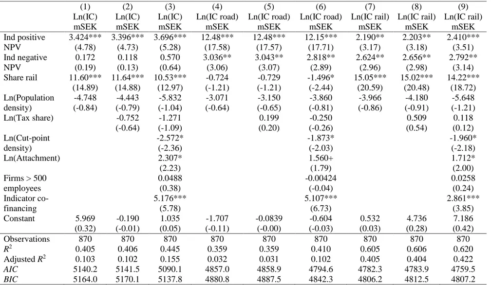
Table 4. Results from a fixed-effects panel regression. (1) (2) (3) (4) (5) (6) (7) (8) (9) Ln(IC) mSEK Ln(IC) mSEK Ln(IC) mSEK Ln(IC road) mSEK Ln(IC road) mSEK Ln(IC road) mSEK Ln(IC rail) mSEK Ln(IC rail) mSEK Ln(IC rail) mSEK Ind positive NPV 3.424*** 3.396*** 3.696*** 12.48*** 12.48*** 12.15*** 2.190** 2.203** 2.410*** (4.78) (4.73) (5.28) (17.58) (17.57) (17.71) (3.17) (3.18) (3.51) Ind negative NPV 0.172 0.118 0.570 3.036** 3.043** 2.818** 2.624** 2.656** 2.792** (0.19) (0.13) (0.64) (3.06) (3.07) (2.89) (2.96) (2.98) (3.14) Share rail 11.60*** 11.64*** 10.53*** -0.724 -0.729 -1.496* 15.05*** 15.02*** 14.22*** (14.89) (14.88) (12.97) (-1.21) (-1.21) (-2.44) (20.59) (20.48) (18.72) Ln(Population density) -4.748 -4.443 -5.832 -3.071 -3.150 -3.860 -3.966 -4.180 -5.648 (-0.84) (-0.79) (-1.04) (-0.64) (-0.65) (-0.81) (-0.86) (-0.91) (-1.21) Ln(Tax share) -0.752 -1.271 0.199 -0.250 0.509 0.118 (-0.64) (-1.09) (0.20) (-0.26) (0.54) (0.12) Ln(Cut-point density) -2.572* -1.873* -1.960* (-2.36) (-2.03) (-2.18) Ln(Attachment) 2.307* 1.560+ 1.712* (2.23) (1.79) (2.00) Firms > 500 employees 0.0488 -0.00424 0.0258 (0.38) (-0.04) (0.24) Indicator co-financing 5.176*** 5.107*** 2.861*** (5.78) (6.73) (3.85) Constant 5.969 -0.190 1.035 -1.707 -0.0839 -0.604 0.532 4.736 7.186 (0.32) (-0.01) (0.05) (-0.11) (-0.00) (-0.03) (0.03) (0.28) (0.42) Observations 870 870 870 870 870 870 870 870 870 R2 _{0.405 0.406 0.445 0.359 0.359 0.410 0.605 0.606 0.620} Adjusted R2 0.103 0.102 0.155 0.032 0.031 0.102 0.405 0.404 0.422 AIC 5140.2 5141.5 5090.1 4857.0 4858.9 4794.6 4782.3 4783.9 4759.5 BIC 5164.0 5170.1 5137.8 4880.8 4887.5 4842.3 4806.2 4812.5 4807.2 t statistics in parentheses + p<0.1, * p<0.05, ** p<0.01, *** p<0.001

The model provides some support for Hypothesis 6. Thus, the existence of a positive NPV in a municipality increases the rate of total investment costs in that municipality by a factor of 3.4 (column (1) of Table 4), road investment costs by a factor of 12.5 (column (4)), and rail

investment costs by a factor of 2.2 (column (7)).

The coefficient for Indicator negative NPV is also significant at 1 % level and positive for road and rail investments. Since we expected a negative NPV to lower investment in those

municipalities, it seems that the mere existence of a NPV measure is sufficient to explain the investment costs of a municipality – whether the measure is positive or negative does not matter. It is nevertheless worth noting that the coefficient in column (1), for the total IC model, is insignificant, and the impact of a negative NPV is much smaller on road investments than the impact of a positive NPV – a negative NPV raises investment in roads by a factor of about 3.0, while a positive NPV raises it by a factor of 12.5. For rail investments (column (7)) the impact is higher for the negative NPV measure, however. F-tests of equal coefficients indicate that the coefficient for Indicator positive NPV on road exceeds the coefficient for Indicator negative NPV on road in a statistically significant manner, but that the coefficients for Indicator positive NPV on rail and Indicator negative NPV on rail are equal to one another.

The second model to test is the district-demand hypothesis (Hypothesis 1). We run the following model: (20) 𝐿𝑛(𝐼𝐶_𝑗𝑡) = 𝛼 + 𝛽₁𝐼𝑛𝑑 𝑝𝑜𝑠 𝑁𝑃𝑉_𝑗𝑡+ 𝛽₂𝐼𝑛𝑑 𝑛𝑒𝑔 𝑁𝑃𝑉_𝑗𝑡+ 𝛿₁𝐿𝑛(𝑇𝑎𝑥 𝑠ℎ𝑎𝑟𝑒_𝑗𝑡) + ∑ 𝛾𝑖𝑥𝑖𝑗𝑡 2 𝑖=1 + 𝜖𝑗𝑡,

The results from the model estimation are shown in columns (2), (5) and (8) in Table 4. The coefficient of Ln(Tax share) is insignificant both for the total IC model and for IC in road and rail. We therefore reject Hypothesis 1.

In order to test the swing-voter with lobbying model we run the following:

(21) 𝐿𝑛(𝐼𝐶𝑗𝑡) = 𝛼 + 𝛽1𝐼𝑛𝑑 𝑝𝑜𝑠 𝑁𝑃𝑉𝑗𝑡+ 𝛽2𝐼𝑛𝑑 𝑛𝑒𝑔 𝑁𝑃𝑉𝑗𝑡+ 𝛿1𝐿𝑛(𝑇𝑎𝑥 𝑠ℎ𝑎𝑟𝑒𝑗𝑡) + 𝜃1𝐿𝑛(𝐶𝑃𝐷𝑗𝑡) + 𝜃2𝐿𝑛(𝐴𝑡𝑡𝑎𝑐ℎ𝑚𝑒𝑛𝑡𝑗𝑡) + 𝜃₃𝐹𝑖𝑟𝑚𝑠500 𝑒𝑚𝑝𝑙𝑜𝑦𝑒𝑒𝑠_𝑗𝑡+ 𝜃₄𝐼𝑛𝑑 𝑐𝑜𝑓𝑖𝑛_𝑗𝑡+ ∑ 𝛾_𝑖𝑥_𝑖𝑗𝑡 2 𝑖=1 + 𝜖_𝑗𝑡.

The results are shown in columns (3), (6) and (9) of Table 4. The swing voter model cannot predict the sign for Ln(Tax share). The coefficient of Ln(Attachment), used to test Hypothesis 2, gets a coefficient that is significant at least at 10 % level of significance in all three models, but it has the “wrong” sign; that is, the coefficient is positive and not negative as conjectured. We therefore reject Hypothesis 2. A similar observation applies to Ln(Cut-point density), which gets a significant sign at 5 % level in all three models, but with a negative sign and not a positive sign as expected. We reject Hypothesis 3 as well.

As explained above, we test Hypothesis 4, which is about the influence of interest groups, by including two variables. One is a measure of the number of firms large enough to have resources for lobbying, namely more than 500 employees. The coefficient for this variable is insignificant in all three models. The other variable measures lobbying mainly by the

municipalities themselves, namely co-financing. The coefficient for the indicator variable is significant at 0.1 % level of significance and takes the expected positive sign in all three models.

Thus, the rate of total IC in a municipality increases by a factor of 5.2 in those municipalities that offer co-financing as compared to municipalities that do not co-finance. The impact on IC on road is an increase by a factor of about 5.1, and on IC on rail by a factor of about 2.9.

Finally, the measures of fit, AIC and BIC, indicate that the district demand model (columns (2), (5) and (8)) offers the worst fit, while the swing-voter with lobbying model (columns (3), (6) and (9)) offers the best fit. The adjusted R2 _{measures support this finding.}

In order to test Hypothesis 5, that spillover effects to neighboring municipalities may explain the investment cost in a municipality, we use cross sections of the data for the respective plans, 2004-15, 2010-21 and 2014-25. Neither Stata nor OpenGeoDa can test spatial correlation in panel data. We estimate the following types of models testing both the district demand model and the swing voter model against the influence of “welfare only”:

(22) 𝐿𝑛(𝐼𝐶_𝑗𝑡) = 𝛼 + 𝜌𝑾𝐿𝑛(𝐼𝐶_𝑗𝑡) + 𝛽₁𝐼𝑛𝑑 𝑝𝑜𝑠 𝑁𝑃𝑉_𝑗𝑡+ 𝛽₂𝐼𝑛𝑑 𝑛𝑒𝑔 𝑁𝑃𝑉_𝑗𝑡 + 𝛿₁𝐿𝑛(𝑇𝑎𝑥 𝑠ℎ𝑎𝑟𝑒_𝑗𝑡) + 𝜃₁𝐿𝑛(𝐶𝑃𝐷_𝑗𝑡) + 𝜃₂𝐿𝑛(𝐴𝑡𝑡𝑎𝑐ℎ𝑚𝑒𝑛𝑡_𝑗𝑡) + 𝜃3𝐹𝑖𝑟𝑚 > 500 𝑒𝑚𝑝𝑙𝑜𝑦𝑒𝑒𝑠𝑗𝑡+ 𝜃4𝐼𝑛𝑑 𝑐𝑜𝑓𝑖𝑛𝑗𝑡+ ∑ 𝛾𝑖𝑥𝑖𝑗𝑡 2 𝑖=1 + 𝜖𝑗𝑡. 𝜖_𝑗𝑡= 𝜆𝑾𝜖_𝑗𝑡+ 𝜇

We start by examining whether the cross sectional data exhibits either heteroscedasticity or spatial autocorrelation. In order to do this, we estimate Equations (19) to (21) using an ordinary least squares (OLS) estimator. We do not show the results in this paper. The Breusch-Pagan test does not indicate heteroscedasticity for total Ln(IC) in 2004, but the models for 2010 and for 2014 are heteroscedastic. The ICs for road and rail regressions are heteroscedastic. The global

measures for spatial autocorrelation, Moran’s I, indicates spatial autocorrelation for the models for Ln(IC on road) in 2010 and in 2014, and for Ln(IC on rail) in 2010, at least at 5 % level of significance, both excluding and including the swing-voter variables. Including the swing voter with lobbying variables, the test indicates spatial autocorrelation for total Ln(IC) in 2010 at 5 % level, and for 2004 at 10 % level.

We estimate model (22) using an estimator that corrects for a spatial lag in the dependent variable. We do not present models with spatially correlated error terms, or Durbin models controlling for both aspects of spatial dependency, because the coefficient for spatially autocorrelated errors in these models is insignificant.

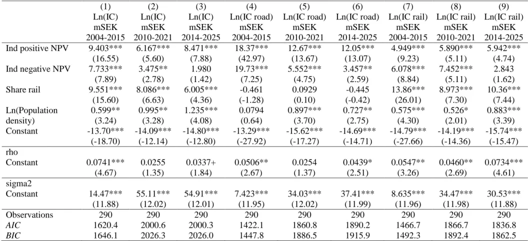
The results for the welfare model (Hypothesis 6, similar to Equation (19)) complemented with the spatial weight matrix) are shown in Table 5. The results with regard to the impact of social welfare (positive NPV) do not change compared to the panel model shown in Table 4. Thus, the impact of welfare considerations is positive for all three plans. It is strongest for road

investments and less so for rail investments.

The results with regard to Indicator negative NPV are similar to the panel model, too, except that the coefficient of the variable is also significant for the total IC model. The above

conclusions hold but Hypothesis 6 cannot be confirmed as it is. Rather than welfare concerns driving the results, it is the mere existence of CBA results that seems to explain project choice.

Table 5. Investment cost per municipality and infrastructure plan explained by concern for social welfare (CBA results), controlling for a spatially lagged dependent variable. The coefficient 𝝆 is included to control for a spatially lagged dependent variable

(1) (2) (3) (4) (5) (6) (7) (8) (9) Ln(IC) mSEK 2004-2015 Ln(IC) mSEK 2010-2021 Ln(IC) mSEK 2014-2025 Ln(IC road) mSEK 2004-2015 Ln(IC road) mSEK 2010-2021 Ln(IC road) mSEK 2014-2025 Ln(IC rail) mSEK 2004-2015 Ln(IC rail) mSEK 2010-2021 Ln(IC rail) mSEK 2014-2025 Ind positive NPV 9.403*** 6.167*** 8.471*** 18.37*** 12.67*** 12.05*** 4.949*** 5.890*** 5.942*** (16.55) (5.60) (7.88) (42.97) (13.67) (13.07) (9.23) (5.11) (4.74) Ind negative NPV 7.733*** 3.475** 1.980 19.73*** 5.552*** 3.457** 6.078*** 7.452*** 2.843 (7.89) (2.78) (1.42) (7.25) (4.75) (2.59) (8.84) (5.11) (1.62) Share rail 9.551*** 8.086*** 6.005*** -0.461 0.0929 -0.445 13.86*** 8.973*** 10.36*** (15.60) (6.63) (4.36) (-1.28) (0.10) (-0.42) (26.01) (7.30) (7.44) Ln(Population density) 0.599** 0.995** 1.235*** 0.0794 0.897*** 0.727** 0.575*** 0.526* 0.883*** (3.24) (3.28) (4.08) (0.64) (3.70) (2.75) (4.30) (2.01) (3.39) Constant -13.70*** -14.09*** -14.80*** -13.29*** -15.62*** -14.69*** -14.79*** -14.19*** -15.74*** (-18.70) (-12.14) (-12.80) (-27.92) (-17.27) (-14.71) (-27.66) (-14.36) (-15.47) rho Constant 0.0741*** 0.0255 0.0337+ 0.0506** 0.0254 0.0439* 0.0547** 0.0460** 0.0734*** (4.67) (1.35) (1.84) (2.67) (1.37) (2.51) (3.26) (2.69) (4.61) sigma2 Constant 14.47*** 55.11*** 54.91*** 7.423*** 34.03*** 37.41*** 8.635*** 34.47*** 30.53*** (11.88) (12.02) (12.01) (11.95) (12.02) (11.99) (11.96) (11.98) (11.88) Observations 290 290 290 290 290 290 290 290 290 AIC 1620.4 2000.6 2000.3 1422.1 1860.8 1890.2 1466.7 1866.7 1836.8 BIC 1646.1 2026.3 2026.0 1447.8 1886.5 1915.9 1492.3 1892.4 1862.5 t statistics in parentheses + p<0.1, * p<0.05, ** p<0.01, *** p<0.001

Spatial spillovers also fare fairly well in explaining the pattern of investment. The 𝜌-coefficient is significant at least at 10 % level for total IC in 2004 and 2014, for road investment in 2004 and 2014, and for rail investment in all three plans. We conclude that spatial spillovers, at least when only controlling for the welfare aspects of project choice, are a significant explanation for the IC in a municipality, and that we cannot reject Hypothesis 5.

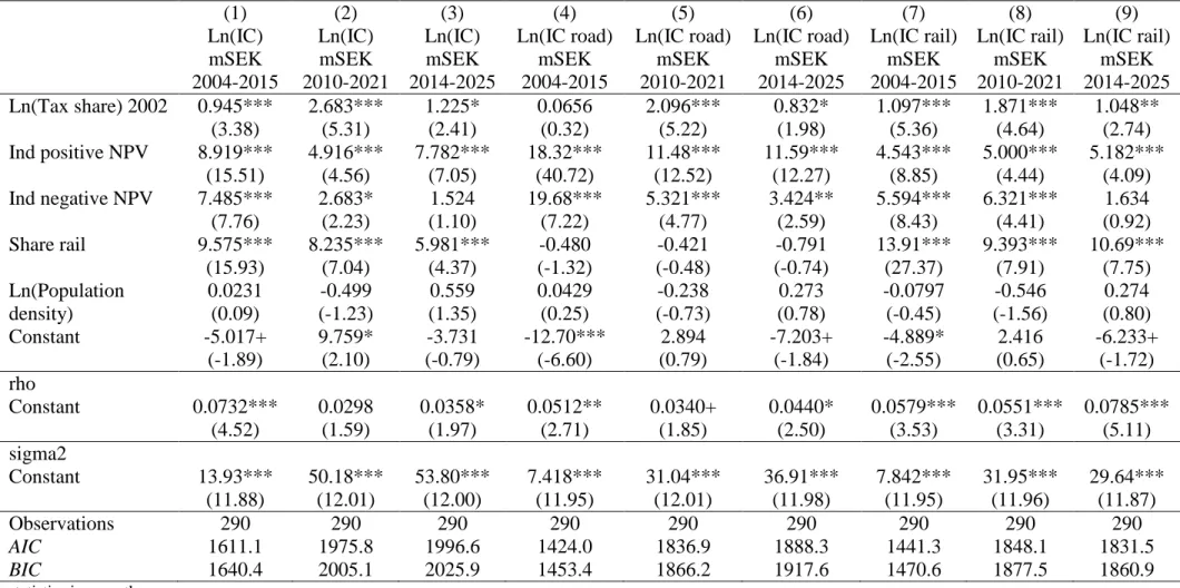
The results from testing the district demand model (Hypothesis 1, similar to Equation (20) with the spatial weight matrix included) are shown in Table 6. The coefficient of Ln(Tax share) is significant in most models but takes the wrong sign. We conclude that we find no support for the district demand model.

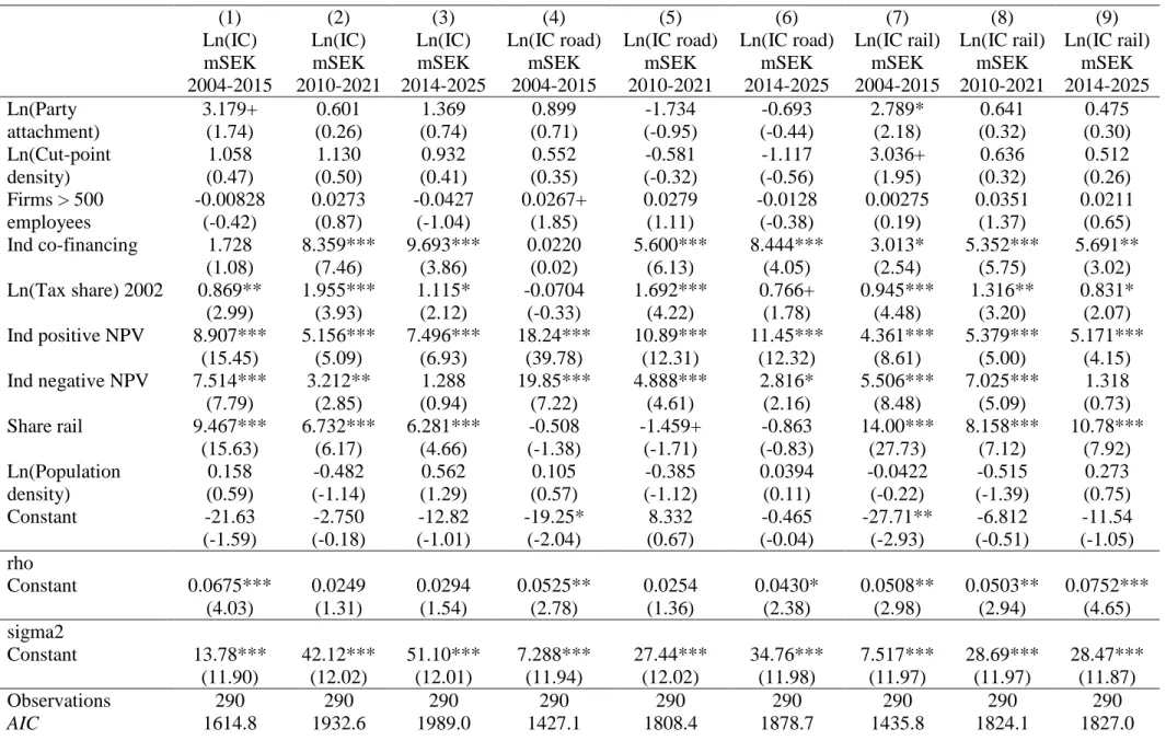
Finally, the results from testing the swing voter model with lobbying (Hypotheses 2-4, the entire model in Equation (22)), including a spatial aspect, are shown in Table 7. The two swing voter variables, Ln(Attachment) and Ln(CPD) either get insignificant coefficients at 5 % level in all nine models, or the coefficient takes the ‘wrong’ sign (column (7)). We thus reject hypotheses 2 and 3 and conclude that when a spatial aspect is added to the list of explanations for infrastructure investment in municipalities, neither political economic hypothesis has explanatory power with regard to the investment volume.

Table 6. The district-demand model tested with an estimator controlling for a spatially lagged dependent variable (1) (2) (3) (4) (5) (6) (7) (8) (9) Ln(IC) mSEK 2004-2015 Ln(IC) mSEK 2010-2021 Ln(IC) mSEK 2014-2025 Ln(IC road) mSEK 2004-2015 Ln(IC road) mSEK 2010-2021 Ln(IC road) mSEK 2014-2025 Ln(IC rail) mSEK 2004-2015 Ln(IC rail) mSEK 2010-2021 Ln(IC rail) mSEK 2014-2025 Ln(Tax share) 2002 0.945*** 2.683*** 1.225* 0.0656 2.096*** 0.832* 1.097*** 1.871*** 1.048** (3.38) (5.31) (2.41) (0.32) (5.22) (1.98) (5.36) (4.64) (2.74) Ind positive NPV 8.919*** 4.916*** 7.782*** 18.32*** 11.48*** 11.59*** 4.543*** 5.000*** 5.182*** (15.51) (4.56) (7.05) (40.72) (12.52) (12.27) (8.85) (4.44) (4.09) Ind negative NPV 7.485*** 2.683* 1.524 19.68*** 5.321*** 3.424** 5.594*** 6.321*** 1.634 (7.76) (2.23) (1.10) (7.22) (4.77) (2.59) (8.43) (4.41) (0.92) Share rail 9.575*** 8.235*** 5.981*** -0.480 -0.421 -0.791 13.91*** 9.393*** 10.69*** (15.93) (7.04) (4.37) (-1.32) (-0.48) (-0.74) (27.37) (7.91) (7.75) Ln(Population density) 0.0231 -0.499 0.559 0.0429 -0.238 0.273 -0.0797 -0.546 0.274 (0.09) (-1.23) (1.35) (0.25) (-0.73) (0.78) (-0.45) (-1.56) (0.80) Constant -5.017+ 9.759* -3.731 -12.70*** 2.894 -7.203+ -4.889* 2.416 -6.233+ (-1.89) (2.10) (-0.79) (-6.60) (0.79) (-1.84) (-2.55) (0.65) (-1.72) rho Constant 0.0732*** 0.0298 0.0358* 0.0512** 0.0340+ 0.0440* 0.0579*** 0.0551*** 0.0785*** (4.52) (1.59) (1.97) (2.71) (1.85) (2.50) (3.53) (3.31) (5.11) sigma2 Constant 13.93*** 50.18*** 53.80*** 7.418*** 31.04*** 36.91*** 7.842*** 31.95*** 29.64*** (11.88) (12.01) (12.00) (11.95) (12.01) (11.98) (11.95) (11.96) (11.87) Observations 290 290 290 290 290 290 290 290 290 AIC 1611.1 1975.8 1996.6 1424.0 1836.9 1888.3 1441.3 1848.1 1831.5 BIC 1640.4 2005.1 2025.9 1453.4 1866.2 1917.6 1470.6 1877.5 1860.9 t statistics in parentheses + p<0.1, * p<0.05, ** p<0.01, *** p<0.001

Table 7. The swing voter with lobbying model tested with an estimator controlling for a spatially lagged dependent variable (1) (2) (3) (4) (5) (6) (7) (8) (9) Ln(IC) mSEK 2004-2015 Ln(IC) mSEK 2010-2021 Ln(IC) mSEK 2014-2025 Ln(IC road) mSEK 2004-2015 Ln(IC road) mSEK 2010-2021 Ln(IC road) mSEK 2014-2025 Ln(IC rail) mSEK 2004-2015 Ln(IC rail) mSEK 2010-2021 Ln(IC rail) mSEK 2014-2025 Ln(Party attachment) 3.179+ 0.601 1.369 0.899 -1.734 -0.693 2.789* 0.641 0.475 (1.74) (0.26) (0.74) (0.71) (-0.95) (-0.44) (2.18) (0.32) (0.30) Ln(Cut-point density) 1.058 1.130 0.932 0.552 -0.581 -1.117 3.036+ 0.636 0.512 (0.47) (0.50) (0.41) (0.35) (-0.32) (-0.56) (1.95) (0.32) (0.26) Firms > 500 employees -0.00828 0.0273 -0.0427 0.0267+ 0.0279 -0.0128 0.00275 0.0351 0.0211 (-0.42) (0.87) (-1.04) (1.85) (1.11) (-0.38) (0.19) (1.37) (0.65) Ind co-financing 1.728 8.359*** 9.693*** 0.0220 5.600*** 8.444*** 3.013* 5.352*** 5.691** (1.08) (7.46) (3.86) (0.02) (6.13) (4.05) (2.54) (5.75) (3.02) Ln(Tax share) 2002 0.869** 1.955*** 1.115* -0.0704 1.692*** 0.766+ 0.945*** 1.316** 0.831* (2.99) (3.93) (2.12) (-0.33) (4.22) (1.78) (4.48) (3.20) (2.07) Ind positive NPV 8.907*** 5.156*** 7.496*** 18.24*** 10.89*** 11.45*** 4.361*** 5.379*** 5.171*** (15.45) (5.09) (6.93) (39.78) (12.31) (12.32) (8.61) (5.00) (4.15) Ind negative NPV 7.514*** 3.212** 1.288 19.85*** 4.888*** 2.816* 5.506*** 7.025*** 1.318 (7.79) (2.85) (0.94) (7.22) (4.61) (2.16) (8.48) (5.09) (0.73) Share rail 9.467*** 6.732*** 6.281*** -0.508 -1.459+ -0.863 14.00*** 8.158*** 10.78*** (15.63) (6.17) (4.66) (-1.38) (-1.71) (-0.83) (27.73) (7.12) (7.92) Ln(Population density) 0.158 -0.482 0.562 0.105 -0.385 0.0394 -0.0422 -0.515 0.273 (0.59) (-1.14) (1.29) (0.57) (-1.12) (0.11) (-0.22) (-1.39) (0.75) Constant -21.63 -2.750 -12.82 -19.25* 8.332 -0.465 -27.71** -6.812 -11.54 (-1.59) (-0.18) (-1.01) (-2.04) (0.67) (-0.04) (-2.93) (-0.51) (-1.05) rho Constant 0.0675*** 0.0249 0.0294 0.0525** 0.0254 0.0430* 0.0508** 0.0503** 0.0752*** (4.03) (1.31) (1.54) (2.78) (1.36) (2.38) (2.98) (2.94) (4.65) sigma2 Constant 13.78*** 42.12*** 51.10*** 7.288*** 27.44*** 34.76*** 7.517*** 28.69*** 28.47*** (11.90) (12.02) (12.01) (11.94) (12.02) (11.98) (11.97) (11.97) (11.87) Observations 290 290 290 290 290 290 290 290 290 AIC 1614.8 1932.6 1989.0 1427.1 1808.4 1878.7 1435.8 1824.1 1827.0

BIC 1658.8 1976.7 2033.1 1471.1 1852.4 1922.8 1479.8 1868.1 1871.0 t statistics in parentheses

40

The lobbying variables Firms > 500 employees and Ind co-financing show an interesting pattern. Thus, the only significant coefficient for the former (at 10 % level) is for road investments in 2004 – a period when co-financing does not seem to have influenced the volume of road investment. Otherwise, it is the coefficient for co-financing which is significant. All the significant coefficients take the expected positive sign. We conclude that we cannot reject Hypothesis 4.

Finally, the 𝜌-coefficient measuring the spatial lag in the dependent variable is significant for the total IC model (column (1) of Table 7), for IC in road in 2004 and 2014 (columns (4) and (6), and for IC in rail in all three Plans. As above, we conclude that we cannot reject Hypothesis 5.

The impact of the two control variables varies between the models. In Table 5, both Share rail and Ln(Population density) get significant coefficients in most of the models, the notable exception for Share rail being the model for Ln(IC on road). Thus, municipalities with a larger share of rail investments out of all investments get more total investment funds and rail

investment funds than municipalities with a lower share of rail investments. Municipalities with higher population density also get more investment funds. This effect disappears in Table 7, however. An explanation for this might be that population density in some way functions as a proxy for co-financing, for instance if municipalities with higher population densities are more prone to co-finance projects. Nevertheless, the two variables are not highly correlated with each other, the correlation coefficient being 0.34 in 2004, 0.25 in 2010 and 0.25 in 2014.