Mä lärdälen University
School of Innovätion Design änd Engineering
Vä sterä s, Sweden
Thesis for the Degree of Master of Science in Computer Science with
Specialization in Embedded Systems 30.0 credits
Real-time Process Modelling Based
on Big Data Stream Learning
Fan He
fhe15001@student.mdh.se
Examiner: Thomas Nolte
Supervisor: Ning Xiong
Table of Contents
1. Introduction ... 1
1.1 Motivation ... 1
1.2 Contribution and Problem Formulation ... 2
1.3 Outline of Thesis ... 2
2. Background ... 3
2.1 Neural Network ... 3
2.1.1 Neuron ... 3
2.1.2 Feedforward Neural Network ... 6
2.2 Recurrent neural network ... 8
2.3 Deep Learning ... 9
2.3.1 Description ... 9
2.3.2 Deep Recurrent Neural Network ... 11
2.4 Existent Training Algorithms ... 11
2.4.1 Backpropagation Through Time ... 12
2.4.2 Extended Kalman filter ... 17
3. Related Work ... 22
4. Research Method ... 23
5. Training Algorithms Comparison ... 24
6. Proposed Training Method ... 26
6.1 Forward Pass... 26
6.2 Hybrid Training Algorithm ... 27
7. Evaluation ... 29 7.1 Static System ... 29 7.1.1 System Identification ... 29 7.1.2 First Experiment ... 30 7.1.3 Second Experiment ... 32 7.2 Time-varying System ... 33 7.2.1 System Identification ... 33 7.2.2 First Experiment ... 34 7.2.3 Second Experiment ... 36 7.3 Discussion ... 37 8. Conclusion ... 38 9. Future Work ... 39 Reference ... 40
Abstract
Most control systems now are assumed to be unchangeable, but this is an ideal situation. In real applications, they are often accompanied with many changes. Some of changes are from environment changes, and some are system requirements. So, the goal of thesis is to model a dynamic adaptive real-time control system process with big data stream. In this way, control system model can adjust itself using example measurements acquired during the operation and give suggestion to next arrival input, which also indicates the accuracy of states under control highly depends on quality of the process model.
In this thesis, we choose recurrent neural network to model process because it is a kind of cheap and fast artificial intelligence. In most of existent artificial intelligence, a database is necessity and the bigger the database is, the more accurate result can be. For example, in case-based reasoning, testcase should be compared with all of cases in database, then take the closer one’s result as reference. However, in neural network, it does not need any big database to support and search, and only needs simple calculation instead, because information is all stored in each connection. All small units called neuron are linear combination, but a neural network made up of neurons can perform some complex and non-linear functionalities. For training part, Backpropagation and Kalman filter are used together. Backpropagation is a widely-used and stable optimization algorithm. Kalman filter is new to gradient-based optimization, but it has been proved to converge faster than other traditional first-order-gradient-based algorithms.
Several experiments were prepared to compare new and existent algorithms under various circumstances. The first set of experiments are static systems and they are only used to investigate convergence rate and accuracy of different algorithms. The second set of experiments are time-varying systems and the purpose is to take one more attribute, adaptivity, into consideration.
Keywords: control system, real-time process, deep learning, recurrent neural network,
List of figures
Figure 1 Biological neuron ... 4
Figure 2 Artificial neuron ... 4
Figure 3 Sigmoid function ... 5
Figure 4 RELU function ... 5
Figure 5 Leaky RELU function ... 6
Figure 6 Feedforward neural network structure ... 7
Figure 7 Basic recurrent neural network structure ... 8
Figure 8 Unrolled recurrent neural network structure ... 9
Figure 9 Deep neural network structure ... 10
Figure 10 Modularization in deep neural network ... 10
Figure 11 Deep recurrent neural network structure ... 11
Figure 12 Gradient descent ... 12
Figure 13 General Backpropagation ... 13
Figure 14 Backpropagation through time ... 15
Figure 15 Kalman filter property ... 17
Figure 16 Research method ... 23
Figure 17 Kalman filter fitness ... 24
Figure 18 BPTT fitness ... 24
Figure 19 Prediction steps ... 26
Figure 20 Training algorithm ... 27
Figure 21 Training algorithm in multi-core processor ... 28
Figure 22 BPTT and Kalman filter result in static system ... 30
Figure 23 Accuracy information of BPTT and Kalman filter in static system ... 30
Figure 24 Proposed algorithm result in static system... 31
Figure 25 Accuracy information of proposed algorithm in static system ... 31
Figure 26 Result of second experiment in static system ... 32
Figure 27 Accuracy information of second experiment in static system ... 32
Figure 28 BPTT and Kalman filter result in time-varying system ... 34
Figure 29 Accuracy information of BPTT and Kalman filter in time-varying system 34 Figure 30 Proposed algorithm result in time-varying system... 35
Figure 31 Accuracy information of proposed algorithm in time-varying system ... 35
Figure 32 Result of second experiment in time-varying system ... 36
Figure 33 Accuracy information of second experiment in time-varying system ... 36
List of Tables
Table 1 Sliding window ... 261
1. Introduction
1.1 Motivation
With the increasing demands of accuracy and prediction, applications and technologies of real-time control systems will be the research trend. They need to process data and perform some predetermined requirements in specified time intervals. [1][2] However, most of models in control systems are designed to learn offline based on training data, [3][4] which means once the model is complete and used, it will not be changed anymore unless the controlled plant is out of service. But in real applications, there can be a lot of changes during operation, so it is necessary to model a real-time control system process. There are two key tasks in a real-time control system to get optimal control. First is constructing the process model used in real-time system to forecast future states. And second is setting control variables dynamically based on prediction results to get expected behavior. Obviously, the accuracy of states under control highly depends on quality of the process model. Since adaptive feedback control process is from simulation of human operation, some researchers try to use Artificial Neural Network (ANN), which mimics a biological brain in a computational way and solves problem like humans do in real life.
ANN has been one hot research topic of artificial intelligence since 1980s. Over the past decade, ANN has got great development in solving pattern recognition, automation, biology and other difficult practical problems. Inspired by biological neural network, an ANN is groups of connected small processing units called artificial neuron and they form an abstract oriented network. Input signal propagates through network in the direction of connection. In contrast with biological neural network, connections between artificial neurons are not added or removed. They are weighted instead and weights are updated using learning algorithms. In supervised learning, learning algorithm adjusts weights and tries to minimize error between prediction output and desired output provided by training examples. [5]
A complete artificial neural network often refers to many training examples. This is the reason we choose a big data stream to train the network so that it can continually change the network all the time to adapt to changes in the system. Big data has been another hot research topic in the past ten years. It can be used in predictive analytics or other advanced data analytics, because large amount of data can help to get more accurate or expected outcomes undoubtedly. The term of big data has been used since 1990s. Big data is usually described by its characteristics. Laney was the first to define data growth challenges and opportunities with three dimensions: Volume, Velocity and Variety, known as 3V's of data. [6] Additional V's have been added by some organizations over ten years, like variability and veracity. [7]
2
1.2 Contribution and Problem Formulation
The aim of thesis is to design and implement a prototype self-learning prediction system with big data stream in a real-time process control framework so that the predicted future states can be used to predict next arrival input or modify the actual arrival input because of noise and other uncertainties. In this way, the response of a control system can be quicker and the dynamic process can be smoother. By self-learning, we mean the update of the model using example measurements acquired during the operation. In other words, the system adjust itself based on history information to predict future states and get better input and all desired inputs and outputs are from a data stream which can be a big data stream or an infinite data stream.
Since no one did some similar things before, the following research points should be considered in thesis.
1. Is neural network suitable for online mode in control system modeling? If the answer is yes, how to apply it to data stream learning?
Since neural network has been proved to be efficient in most offline real applications, only few researchers tried it in a dynamic way. This should be validated first because it is the base of using neural network to model the real-time control system process. Offline learning and online learning are completely different in design. A new way should be developed for online training.
2. What are differences among existing training algorithms? Can they all be used in online learning?
Training is the most difficult part in neural network modeling, because the structure is settled and the only difference between two neural networks is the choice of training method. So, we need to investigate them and know what are pros and cons of each one. 3. Can neural network be fast enough in a real-time system?
With the increase of data, demand of time will also grow at the same time, but real-time is a time-critical definition. Most real-time systems have hard deadlines and task period is short, so each training phase must be finished and provide high prediction accuracy in a limited time interval. This gives high timing requirements.
1.3 Outline of Thesis
In Section 2, background of neural network is introduced and related work is given in Section 3. Section 4 gives the research methodology used in the thesis. Training algorithms deployed in thesis work are fully detailed in Section 5. Section 6 describes the system model in detail, including prediction and training parts. Evaluation results are presented and discussed in Section 7. Conclusion are drawn and future work is also mentioned at the end.
3
2. Background
In this section, some basic definitions and structures of neural network are introduced, including neuron, feedforward neural network, deep learning and recurrent neural network.
2.1 Neural Network
A neural network is a parallel non-linear system which is composed of huge amount of connected process units. Although functionality of each unit is very simple, the network can still provide various and complex functionalities. This means information is not stored in any specific area. It is stored in every connection instead. In all, distribution and parallelism can bring great fault tolerance. First, because of distribution, if some neurons are broken, they will not degrade overall performance. For example, in real life, there are many nerve cells dying every day, but the human brain can still work well.[8] In artificial neural network, it is the same that part of broken units will not influence overall performance. Second, when input information is not clear or some information is missing, network can still recover the whole memory. Therefore, humans can recognize irregular handwriting.
Another characteristic of neural network is adaptivity. Adaptivity includes self-study and self-organization. Self-study means once environment changes, after a period of training time or perception, network can adjust some internal parameters automatically to give an expected output. And neural network can adjust the connection between two neurons according to certain rules to construct a complete network, which is called self-organization.
2.1.1 Neuron
One human brain consists of 1010 to 1012 units called neurons, which is a huge complex
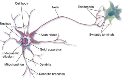
parallel information processing system. Each neuron is connected to other millions of neurons and communicates with them via electrochemical signals. Neuron continuously receives signal via synapses, located at the end of branches as shown in figure 1, and then performs in some specific ways. If the result is greater than the pre-defined threshold value, neuron will fire and generate a voltage and output a signal along something called an axon. [9]
4
Figure 1 Biological neuron
In ANN, network is made up of many artificial neurons. These modelled neurons perform together in similar way to simulate human brain in a math way. The number of neurons can be as small as unit's digit or as big as thousand's digit. Each input into the neuron has its own corresponding weight. A weight is often a floating-point number and it is what to be adjusted when network is trained. Weights in neural network can be both negative and positive and each input is multiplied by its corresponding weight to get linear combination. Inputs and weights can be represented as 𝑥1, 𝑥2… 𝑥𝑛 and 𝑤1, 𝑤2… 𝑤𝑛. So, the linear combination can be written as:
𝑥1𝑤1+ 𝑥2𝑤2+ 𝑥3𝑤3+ ⋯ + 𝑥𝑛𝑤𝑛 = ∑ 𝑥𝑗𝑤𝑗
𝑛
𝑗=0
( 1 )
The following picture is a basic artificial neuron structure.
Figure 2 Artificial neuron
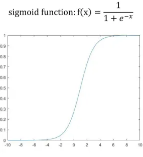
From figure 2, after calculating linear combination, unit gives activation σ, which is generally sigmoid function.
5
sigmoid function: f(x) = 1
1 + 𝑒−𝑥 ( 2 )
Figure 3 Sigmoid function
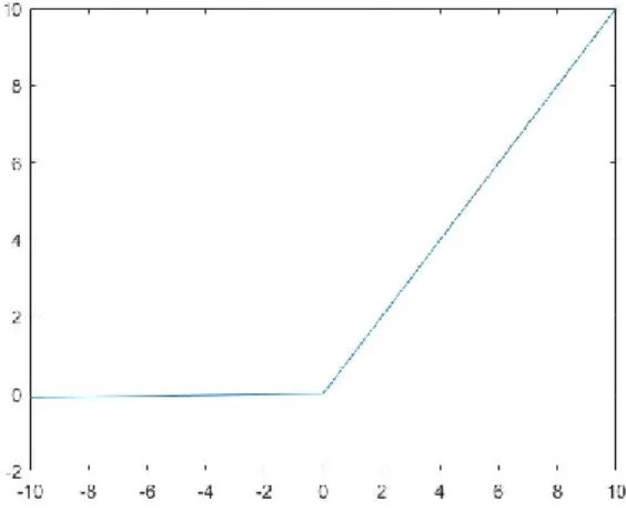
In this project, a new and popular activation function called Rectified Linear Units (RELU) is used.
RELU function: f(x) = max(0, 𝑥) ( 3 )
Figure 4 RELU function
It is from biology with same effect as sigmoid function. It can reduce possibility of vanishing gradient problem when training neural network, especially in deep neural network. And The other benefit of RELU is sparsity. Sparsity means the network can use as few non-zero values as possible to represent extracted features and it arises when linear combination ≤ 0 . The more units exist in a layer, the sparser resulting representation can be. On the other hand, Sigmoid always generates non-zero values to give dense representations. Obviously, sparse representations are more beneficial than dense representations. [10]
However, RELU is not all-mighty. It may be "dead" during training. If absolute value of one dimension of weights is larger than expected, it may cause the weight that the neuron
6
will never activate on any example again, which means the gradient will be zero forever and RELU units will irreversibly die during training. A network will be "dead" with high probability if the learning rate is too high. It is also called "dying RELU" problem. With a proper setting of learning rate, this is less frequently an issue. Or another solution is to use leaky RELU.
Leaky RELU function: f(x) = max (0.01𝑥, 𝑥) ( 4 )
Figure 5 Leaky RELU function
When linear combination < 0, the function output is very small and we can ignore its value to some extent, but in the same time, it also prevents dying RELU problem. Therefore, it is widely used in deep neural network now.
2.1.2 Feedforward Neural Network
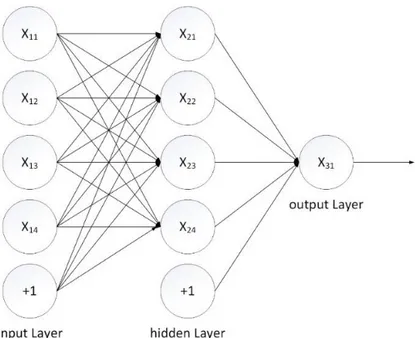
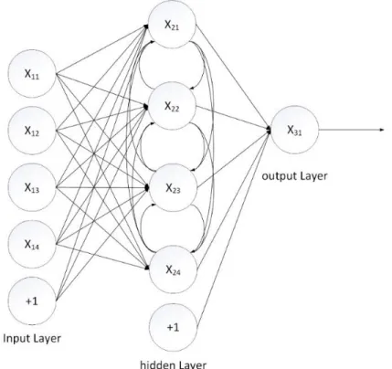
One common way of connecting neurons is to organize neurons into a design called feedforward neural network. It gets its name from the way that neurons in each layer are connected to next layer and feed their output again forward to the third layer until getting final output from neural network. The following is a very simple three-layer feedforward network.
7
Figure 6 Feedforward neural network structure
Each neuron receives input values from the previous layer and sends output to next layer without feedback. All neurons in a network can be categorized in three kinds: input, hidden and output. Input neurons compose input layer. This layer only performs communication and sends information into network. In the same way, output layer consists of output neurons and receives information from network. Input layer and output layer are directly connected to environment, so they are called visible layers as well. Hidden layers, also called middle layers, do not have any relationship with outside. In hidden layers and output layer, every unit has multiple inputs, but only one output, which is also one of the input for next layer. The picture above is a fully-connected network, and each neuron in one layer is connected to all of neurons in the previous layer, including one special neuron whose value equals +1. The special one is for bias and its main functionality is affine transformation. The correct output representation of one neuron should be:
output = σ (1 ∗ 𝑏𝑘+ ∑ 𝑥𝑗𝑤𝑗 𝑛
𝑗=1
) ( 5 )
So, bias is often seen as a part of weights (𝑤0) and corresponding input as +1. This
assumption not only makes structure clear, but also makes calculation less complex. We can see that hidden layers play an important role in a feedforward neural network because they can grab high-order statistical features. The more layers it has, the more valuable this ability can be. To start from the macro-view, a feedforward neural network is a static non-linear mapping system. It obtains powerful non-linear processing ability by some simple non-linear composite mappings.
8
2.2 Recurrent neural network
Unlike feedforward neural network, recurrent neural network (RNN) can use its internal memory to remember and process sequential data. This makes them applicable to time series prediction tasks. [11]
The idea behind RNN is to make use of sequential information. In a traditional feedforward neural network, all inputs, states and outputs are independent of each other. But for many real applications, this is a very bad idea. For example, if you want to predict the next word in a sentence you had better know which words came before. RNN can do this because they perform same tasks on every element of a sequence and they have a "memory" which collects information about what has been calculated so far.
The following case of basic structure was the first RNN by Jeff Elman. A three-layer network was used, with the addition of a set of "context units". There are connections from the hidden layer to these context units fixed with a weight of one. [12]
Figure 7 Basic recurrent neural network structure
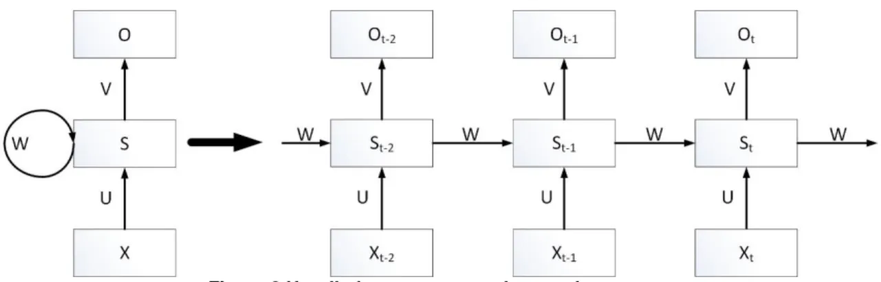
However, the picture above is not a good way to show how it works, so typically, an unrolled diagram is used, as figure 8 shows, where rectangle means a whole layer with several neurons, including bias.
9
Figure 8 Unrolled recurrent neural network structure
By unrolling, it simply means that network can be written with complete sequence. For example, if the sequence is a sentence of 5 words, the network would be unrolled into a 5-layer neural network, one 5-layer for each word.
The key point and difference between RNN and traditional ANN is that output of hidden-layer not only refers to inputs, but also depends on the hidden-hidden-layer states from previous time steps. We can use the following equations to calculate:
𝑜𝑡 = 𝜎(V𝑆𝑡) = 𝜎 (∑ 𝑣𝑘𝑗𝑠𝑗(𝑡) 𝑗
) ( 6 )
𝑆𝑡= 𝜎(𝑈𝑋𝑡+ 𝑊𝑆𝑡−1) ( 7 )
Equation ( 6 ) is calculation of output layer. Each neuron in output layer is connected to all of neurons in last hidden layer, so it is a fully-connected layer. V is weights matrix of output layer. Equation ( 7 ) is calculation of hidden layers, which are recurrent layers. U and W are weights matrixes of input layer and hidden layer at previous time step respectively. There are 3 kinds of recurrent neural network structure for different problems: many-to-one, many-to-many and many-to-many with delay. Many-to-one is used in trend prediction or regression problem. It has totally multiple inputs in different unfolding networks, but only one output. Many-to-many is generally used in typing correction. For example, it is common that someone missed one letter when typing one word or someone do not remember the correct spelling, then the system can detect it and correct it automatically. The third one, many-to-many with delay, is widely used in mobile phones. It is the best solution to word association. Output starts after a complete input words sequence or just one word, then network captures some important information from the input sequence and tells what is the meaning input says and search the most relevant words in database.
2.3 Deep Learning
2.3.1 Description
10
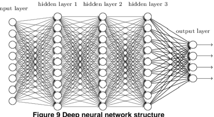
Models consisting of multiple layers of non-linear information processing;
Figure 9 Deep neural network structure
Methods for supervised or unsupervised learning of feature representation at successively higher, more abstract layers.
Deep learning is in the intersections among research areas of neural network and artificial intelligence. Three important reasons why deep learning is so popular now are the greatly increased chip processing abilities, the significantly increased size of training data, and the recent advances in machine learning and information processing research, which have enabled deep learning methods to effectively exploit complex, compositional non-linear functions, to learn hierarchical feature representations. [13]
One traditional deep learning network has the same structure as shallow neural network like figure 9 shows. It can also use a flow graph to show how the calculation works. But one of special attribute is depth, which is the length of the longest path from input layer to output layer. One more hidden layer means more abstract and features can be subdivided. For example, there is a picture and we want to identify whether the person in this picture is a boy or a girl with long or short hair. The following picture shows why a deep network can work better than a one-hidden-layer neural network: [14]
11
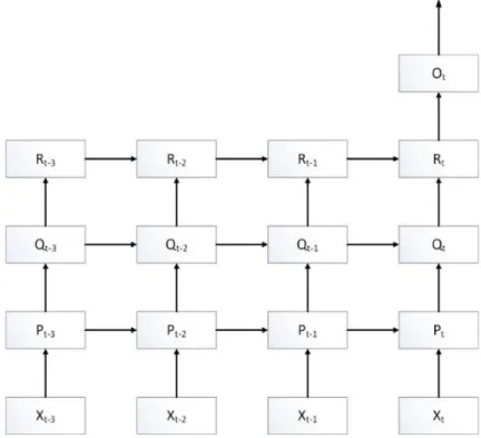
2.3.2 Deep Recurrent Neural Network
Deep recurrent neural network is the final choice in this project. Compared with traditional deep neural network, it has recurrent hidden layers to store history information to deal with sequential problem. And as mentioned before, the more hidden layers there are in a neural network, the stronger the ability that can grab high-order statistical features is. So, it can solve more complex systems and make more precise results than a shallow recurrent neural network. [15]
Figure 11 Deep recurrent neural network structure
2.4 Existent Training Algorithms
To train a recurrent neural network, one of widely-used and efficient method is Backpropagation through time (BPTT) learning algorithm. BPTT comes from Backpropagation algorithm (BP), but it takes time steps into consideration to be applicable to RNN. [24] In this project, another algorithm, Kalman filter, is also used, Since Kalman filter only works for linear system, a compromised method, extended Kalman filter (EKF), is employed to make it combined with gradient and weight,
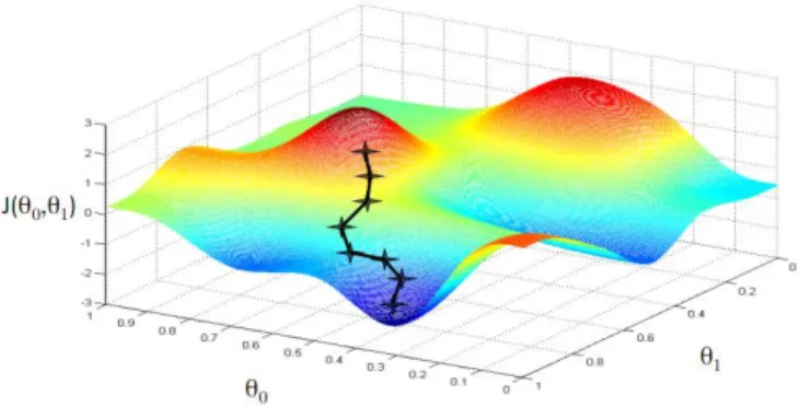
Gradient descent, also known as steepest descent, is a basic idea to minimize a function J(𝜃0, 𝜃1, … , 𝜃𝑛) by updating parameters in the opposite direction of gradient. The learning rate η is the size of steps. In other words, the output is like a ball. It rolls downhill on the surface of function in the direction of slope until reaching valley.
12
Figure 12 Gradient descent
2.4.1 Backpropagation Through Time
2.4.1.1 General Backpropagation
General BP is a basic optimization for feedforward neural network.
Backpropagation steps
1
Initialization: If it is a totally new network, then randomize all of weights. They should be a normal distribution with 0 being mean value and 1 being variance.
2 Provide training examples set {(𝑥(𝑛), 𝑑(𝑛))}𝑛=1𝑁 .
3 Calculate outputs of hidden layers and output layer of each training example. 4 Calculate error between prediction result and desired result and propagate
error signal to each hidden layer.
5 Update all of weights based on error signal.
6 Iteration: Back to step 3 until the network satisfy given rules.
A neural network with the following parameters:
𝑤𝑘𝑗𝑙 means the weight from 𝑘𝑡ℎ neurons in (𝑙 − 1)𝑡ℎ layer to 𝑗𝑡ℎneurons in 𝑙𝑡ℎ layer.
𝑏𝑗𝑙 means the bias for 𝑗𝑡ℎ neurons in 𝑙𝑡ℎ layer.
𝑧𝑗𝑙 means the linear combination of 𝑗𝑡ℎ neurons in 𝑙𝑡ℎ layer:
𝑧𝑗𝑙 = 𝑏𝑗𝑙+ ∑ 𝑤𝑘𝑗𝑙 𝑎𝑘𝑙−1
𝑘
13
𝑎𝑗𝑙 means the output of 𝑗𝑡ℎ neurons in 𝑙𝑡ℎ layer:
𝑎𝑗𝑙 = σ (𝑏𝑗𝑙+ ∑ 𝑤𝑘𝑗𝑙
𝑘
𝑎𝑘𝑙−1) ( 9 )
Backpropagation learning algorithm can be divided into two phases: backward propagation and weight update.
First is backward propagation. We need to define a loss function for output first. Then, propagate error signal back to all output and hidden neurons. A commonly-used loss function is root-mean-square deviation.
E =1
2(𝑦(𝑥) − 𝑎
𝐿(x))2 ( 10 )
x and y are training examples' input and output (desired input and output) respectively. 𝑎𝐿 is the prediction value and L is maximum of layer number.
Figure 13 General Backpropagation
Error term of 𝑗𝑡ℎ neurons in 𝑙𝑡ℎ layer is defined as:
𝛿𝑗𝑙 = 𝜕𝐸
𝜕𝑧𝑗𝑙 ( 11 ) So, the error term of last (output) layer is:
𝛿𝐿 = 𝜕𝐸 𝜕𝑧𝑗𝐿 = 𝜕𝐸 𝜕𝑎𝑗𝐿 𝜕𝑎𝑗𝐿 𝜕𝑧𝑗𝐿 = 𝜕𝐸 𝜕𝑎𝐿𝜎′(𝑧 𝐿) ( 12 )
14
Then, based on the calculated error term of last (output) layer, calculate other error terms backward layer by layer.
𝛿𝑗𝑙= 𝜕𝐸 𝜕𝑧𝑗𝑙 = ∑ 𝜕𝐸 𝜕𝑧𝑚𝑙+1 𝜕𝑧𝑚𝑙+1 𝜕𝑎𝑗𝑙 𝜕𝑎𝑗𝑙 𝜕𝑧𝑗𝑙 𝑚 = 𝛿𝑚𝑙+1 𝜕(𝑏𝑚𝑙+1+ ∑ 𝑤𝑚 𝑗𝑚𝑙+1∗ 𝑎𝑗𝑙) 𝜕𝑎𝑗𝑙 𝜎 ′(𝑧 𝑗𝑙) = ∑ 𝛿𝑚𝑙+1𝑤 𝑗𝑚𝑙+1𝜎′(𝑧𝑗𝑙) 𝑚 ( 13 )
After calculating all of neurons' error terms, the next step is calculating each bias. 𝜕𝐸 𝜕𝑏𝑗𝑙= 𝜕𝐸 𝜕𝑧𝑗𝑙 𝜕𝑧𝑗𝑙 𝜕𝑏𝑗𝑙 = 𝛿𝑗 𝑙𝜕(𝑏𝑗 𝑙+ ∑ 𝑤 𝑘𝑗𝑙 𝑎𝑘𝑙−1 𝑘 ) 𝜕𝑏𝑗𝑙 = 𝛿𝑗 𝑙 ( 14 )
And each dimension of weights. 𝜕𝐸 𝜕𝑤𝑘𝑗𝑙 = 𝜕𝐸 𝜕𝑧𝑗𝑙 𝜕𝑧𝑗𝑙 𝜕𝑤𝑘𝑗𝑙 = 𝛿𝑗 𝑙𝜕(𝑏𝑗 𝑙+ ∑ 𝑤 𝑘𝑗𝑙 𝑎𝑘𝑙−1 𝑘 ) 𝜕𝑤𝑘𝑗𝑙 = 𝛿𝑗 𝑙𝑎 𝑘𝑙−1 ( 15 )
The third phase is weight update.
{ 𝑤𝑘𝑗𝑙 − ∇𝑤 𝑘𝑗𝑙 = 𝑤𝑘𝑗𝑙 − 𝜂 𝜕𝐸 𝜕𝑤𝑘𝑗𝑙 𝑏𝑗𝑙− ∇𝑏𝑗𝑙= 𝑏𝑗𝑙− 𝜂𝜕𝐸 𝜕𝑏𝑗𝑙 ( 16 )
2.4.1.2 Backpropagation Through Time
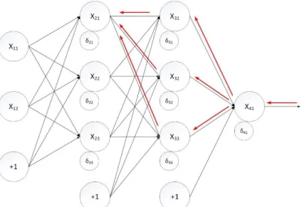
BPTT do same things but do not only backpropagate to input layer but also to hidden layers in previous time steps to update weights. The following pictures simply shows how error signal is propagated through each hidden layer at different time steps.
15
Figure 14 Backpropagation through time
𝑤𝑘𝑗𝑙 means the weight from 𝑘𝑡ℎ neurons in (𝑙 − 1)𝑡ℎ layer to 𝑗𝑡ℎneurons in 𝑙𝑡ℎ layer.
𝑣𝑖𝑗𝑙 means the weight from 𝑖𝑡ℎ neurons in 𝑙𝑡ℎ layer in unfolding 𝑢 + 1𝑡ℎ time to
𝑗𝑡ℎneurons in 𝑙𝑡ℎ layer at unfolding 𝑢𝑡ℎ time. 𝑏𝑗𝑙 means the bias of 𝑗𝑡ℎ neurons in 𝑙𝑡ℎ layer.
𝑧𝑗𝑢𝑙 means linear combination of 𝑗𝑡ℎ neurons in 𝑙𝑡ℎ layer at unfolding 𝑢𝑡ℎ time.
{ 𝑧𝑗𝑢𝑙 = 𝑏𝑗𝑙+ ∑ 𝑤𝑘𝑗𝑙 𝑎𝑘𝑢𝑙−1 𝑘 + ∑ 𝑣𝑖𝑗𝑙𝑎𝑖,𝑢+1𝑙 𝑖 , u < U 𝑧𝑗𝑢𝑙 = 𝑏𝑗𝑙+ ∑ 𝑤𝑘𝑗𝑙 𝑎𝑘𝑢𝑙−1 𝑘 , u = U ( 17 )
𝑎𝑗𝑢𝑙 means the output for 𝑗𝑡ℎ neurons in 𝑙𝑡ℎ layer at unfolding 𝑢𝑡ℎ time.
{ 𝑎𝑗𝑢𝑙 = σ (𝑏 𝑗𝑙+ ∑ 𝑤𝑘𝑗𝑙 𝑎𝑘𝑢𝑙−1 𝑘 + ∑ 𝑣𝑖𝑗𝑙 𝑎𝑖,𝑢+1𝑙 𝑖 ) , u < U 𝑎𝑗𝑢𝑙 = σ (𝑏𝑗𝑙+ ∑ 𝑤𝑘𝑗𝑙 𝑎𝑘𝑢𝑙−1 𝑘 ) , u = U ( 18 )
16
The error term of last (output) layer is the same as BP because output layer is not a recurrent layer: 𝛿𝐿 = 𝜕𝐸 𝜕𝑧𝑗𝐿 = 𝜕𝐸 𝜕𝑎𝑗𝐿 𝜕𝑎𝑗𝐿 𝜕𝑧𝑗𝐿 = 𝜕𝐸 𝜕𝑎𝐿𝜎′(𝑧 𝐿) ( 19 )
Then, based on the error term of last (output) layer, we can calculate other error terms backward layer by layer.
𝛿𝑗𝑢𝑙 = 𝜕𝐸 𝜕𝑧𝑗𝑢𝑙 = ∑ 𝜕𝐸 𝜕𝑧𝑚𝑢𝑙+1∗ 𝜕𝑧𝑚𝑢𝑙+1 𝜕𝑎𝑗𝑢𝑙 ∗ 𝜕𝑎𝑗𝑢𝑙 𝜕𝑧𝑗𝑢𝑙 + ∑ 𝜕𝐸 𝜕𝑧𝑛,𝑢−1𝑙 ∗ 𝜕𝑧𝑛,𝑢−1𝑙 𝜕𝑎𝑗𝑢𝑙 ∗ 𝜕𝑎𝑗𝑢𝑙 𝜕𝑧𝑗𝑢𝑙 𝑛 𝑚 = 𝛿𝑚𝑢𝑙+1𝜕(𝑏𝑚 𝑙+1+ ∑ 𝑤 𝑗𝑚𝑙+1∗ 𝑎𝑗𝑢𝑙 𝑚 + ∑ 𝑣𝑔 𝑔𝑚𝑙+1∗ 𝑎𝑔,𝑢+1𝑙+1 ) 𝜕𝑎𝑗𝑢𝑙 σ ′(𝑧 𝑗𝑢𝑙 ) + 𝛿𝑛,𝑢−1𝑙 𝜕(𝑏𝑛 𝑙 + ∑ 𝑤 ℎ𝑛𝑙 ∗ 𝑎ℎ,𝑢−1𝑙−1 ℎ + ∑ 𝑣𝑛 𝑗𝑛𝑙 ∗ 𝑎𝑗𝑢𝑙 ) 𝜕𝑎𝑗𝑢𝑙 𝜎′(𝑧𝑗𝑢𝑙 ) = ∑ 𝛿𝑚𝑢𝑙+1𝑤𝑗𝑚𝑙+1𝜎′(𝑧𝑗𝑢𝑙 ) 𝑚 + ∑ 𝛿𝑛,𝑢−1𝑙 𝑣𝑗𝑛𝑙 𝜎′(𝑧𝑗𝑢𝑙 ) 𝑛 , u > 1 ( 20 ) 𝛿𝑗𝑢𝑙 = 𝜕𝐸 𝜕𝑧𝑗𝑢𝑙 = ∑ 𝜕𝐸 𝜕𝑧𝑚𝑢𝑙+1∗ 𝜕𝑧𝑚𝑢𝑙+1 𝜕𝑎𝑗𝑢𝑙 ∗ 𝜕𝑎𝑗𝑢𝑙 𝜕𝑧𝑗𝑢𝑙 𝑚 = 𝛿𝑚𝑢𝑙+1𝜕(𝑏𝑚 𝑙+1+ ∑ 𝑤 𝑗𝑚𝑙+1∗ 𝑎𝑗𝑢𝑙 𝑚 + ∑ 𝑣𝑔 𝑔𝑚𝑙+1∗ 𝑎𝑔,𝑢+1𝑙+1 ) 𝜕𝑎𝑗𝑢𝑙 σ′(𝑧𝑗𝑢𝑙 ) = ∑ 𝛿𝑚𝑡𝑙+1𝑤𝑗𝑚𝑙+1𝜎′(𝑧𝑗𝑢𝑙 ) 𝑚 , u = 1 ( 21 )
After calculating all of neurons' error terms, the next step is calculating each bias. 𝜕𝐸 𝜕𝑏𝑗𝑢𝑙 = 𝜕𝐸 𝜕𝑧𝑗𝑢𝑙 𝜕𝑧𝑗𝑢𝑙 𝜕𝑏𝑗𝑙 = 𝛿𝑗𝑢𝑙 𝜕(𝑏𝑗𝑙+ ∑ 𝑤𝑘 𝑘𝑗𝑙 𝑎𝑘𝑢𝑙−1+ ∑ 𝑣𝑖 𝑖𝑗𝑙𝑎𝑖,𝑢+1𝑙 ) 𝜕𝑏𝑗𝑙 = 𝛿𝑗𝑢𝑙 ( 22 )
17 𝜕𝐸 𝜕𝑤𝑘𝑗𝑢𝑙 = 𝜕𝐸 𝜕𝑧𝑗𝑢𝑙 𝜕𝑧𝑗𝑢𝑙 𝜕𝑤𝑘𝑗𝑙 = 𝛿𝑗𝑢𝑙 𝜕(𝑏𝑗 𝑙+ ∑ 𝑤 𝑘𝑗𝑙 𝑎𝑘𝑢𝑙−1 𝑘 + ∑ 𝑣𝑖 𝑖𝑗𝑙𝑎𝑖,𝑢+1𝑙 ) 𝜕𝑤𝑘𝑗𝑙 = 𝛿𝑗𝑡𝑙𝑎𝑘𝑢𝑙−1 ( 23 ) 𝜕𝐸 𝜕𝑣𝑖𝑗𝑢𝑙 = 𝜕𝐸 𝜕𝑧𝑗𝑢𝑙 𝜕𝑧𝑗𝑢𝑙 𝜕𝑣𝑖𝑗𝑙 = 𝛿𝑗𝑢 𝑙 𝜕(𝑏𝑗 𝑙+ ∑ 𝑤 𝑘𝑗𝑙 𝑎𝑘𝑢𝑙−1 𝑘 + ∑ 𝑣𝑖 𝑖𝑗𝑙𝑎𝑖,𝑢+1𝑙 ) 𝜕𝑣𝑖𝑗𝑙 = 𝛿𝑗𝑡𝑙𝑎𝑖,𝑢+1𝑙 ( 24 )
The third phase is weight update.
{ 𝑤𝑘𝑗𝑙 − ∇𝑤𝑘𝑗𝑙 = 𝑤𝑘𝑗𝑙 − 𝜂 ∑ 𝜕𝐸 𝜕𝑤𝑘𝑗𝑢𝑙 𝑢 𝑣𝑖𝑗𝑙 − ∇𝑣𝑖𝑗𝑙 = 𝑣𝑖𝑗𝑙 − 𝜂 ∑ 𝜕𝐸 𝜕𝑣𝑖𝑗𝑢𝑙 𝑢 𝑏𝑗l− ∇𝑏𝑗𝑙 = 𝑏𝑗𝑙− 𝜂 ∑ 𝜕𝐸 𝜕𝑏𝑗𝑢𝑙 𝑢 ( 25 )
2.4.2 Extended Kalman filter
Kalman filter is an algorithm that uses states from previous time steps, inputs at current time step and noise (typically Gaussian noise) to give an estimated state. It has been widely used in dynamic control systems, such as robot, aircraft and spacecraft and so on. Moreover, because of its characteristics, it can also be applicable to time series prediction in communication and economy. The main idea behind Kalman filter is to update states and covariance of states to preliminary guesses by extrapolating from previous values. Then adjust these preliminary guesses by incorporating the information contained in measurements. And the key property of Kalman filter is the product of two Gaussian functions is another Gaussian function. [25]
18
In this thesis, Kalman filter is combined with terms of gradient and weight. However, the original Kalman filter is limited to linear dynamic systems. If the system is non-linear, which is the case of neural network, it will not work. So, we must extend Kalman filter by linearization procedure, which is called extended Kalman filter (EKF). [26][27] To apply EKF to the task of estimating weights of neural network, we need to see weights as states in dynamic systems. To start from the macro-view, the network is like:
output = h(w, input(0,1, … , n)) ( 26 ) If we render function h a time-dependent function ℎ𝑛, it will become what we need, a
function between weights and output, which can be transformed into input and output in EKF:
output = ℎ𝑛(𝑤(𝑛)) ( 27 ) There are only 2 phases in Kalman filter, predict and update.
Predict
1. Predict current state based on the previous state and current input.
𝑥̂ = 𝐹𝑡|𝑡−1 𝑡𝑥𝑡−1|𝑡−1̂ + 𝐵𝑡𝑢𝑡 ( 28 ) Where:
● t is the time step.
● 𝑥𝑡 is the state containing the terms of interest for the system. In neural network training, it represents weight.
● 𝐹𝑡 is the state transition matrix. In neural network training, since weights are
assumed to be equal when they are at 𝑡𝑡ℎ time step and 𝑡 − 1𝑡ℎ time step, so 𝐹𝑡 is
identity matrix.
● 𝐵𝑡 is the control input matrix which applies the effect of each control input. For weights in neural network, there is no input, so 𝐵𝑡 is 0.
● 𝑢𝑡 is is the control input. We do not need new input for training. 2. Predict covariance.
𝑃𝑡|𝑡−1= 𝐹𝑡𝑃𝑡−1|𝑡−1𝐹𝑡𝑇+ 𝑄𝑡 ( 29 )
Where:
● 𝑃𝑡 is the covariance matrix which stores variances and covariances of states (weights).
19
● 𝑄𝑡 is the process noise covariance matrix of noisy control inputs
Update
1. Calculate covariance of residual
𝑆𝑡= 𝐻𝑡𝑃𝑡|𝑡−1𝐻𝑡𝑇+ 𝑅𝑡 ( 30 )
𝐻𝑡 is the transformation matrix that maps states into measurements. This is the only
difference in training neural network between original Kalman filter and EKF. In original Kalman filter, measurements of the linear system can be described as
𝑧𝑡 = 𝐻𝑡𝑥𝑡+ 𝑣𝑡, 𝑣𝑡~𝑁(0, 𝑅𝑡) ( 31 ) Where 𝑅𝑡 is the measurement noise covariance.
By contrast, in EKF, the measurement model need not be linear functions of states but non-linear functions instead.
𝑧𝑡 = ℎ(𝑥𝑡) + 𝑣𝑡, 𝑣𝑡~𝑁(0, 𝑅𝑡) ( 32 )
It is obvious that function h cannot be applied to covariance calculation directly. Instead, a matrix of partial derivatives is computed. The basic idea is linearization of the latest state estimate ℎ(𝑥𝑡). The first-order Taylor series is used to make it linearized.
ℎ(𝑥𝑡) ≈ h(𝜇̅) + h′(𝜇̅)(𝑥𝑡− 𝜇̅ ) = h(𝜇̅) + 𝐻𝑡 𝑡(𝑥𝑡− 𝜇̅ ) 𝑡 ( 33 )
In BP, Gradient is partial derivative of error with respect to each weight, but in EKF, it should be partial derivative of output with respect to each weight 𝐻𝑡= 𝜕ℎ(𝑥𝑡)
𝜕𝑥 . So,
the error term of output layer is replaced with "output term":
𝛾𝐿 = 𝜕ℎ 𝜕𝑧𝑗𝐿 = 𝜕ℎ 𝜕𝑎𝑗𝐿 𝜕𝑎𝑗𝐿 𝜕𝑧𝑗𝐿 = 𝜕ℎ 𝜕𝑎𝐿𝜎′(𝑧 𝐿) ( 34 )
20 𝛾𝑗𝑢𝑙 = 𝜕ℎ 𝜕𝑧𝑗𝑢𝑙 = ∑ 𝜕ℎ 𝜕𝑧𝑚𝑢𝑙+1 ∗𝜕𝑧𝑚𝑢 𝑙+1 𝜕𝑎𝑗𝑢𝑙 ∗ 𝜕𝑎𝑗𝑢𝑙 𝜕𝑧𝑗𝑢𝑙 + ∑ 𝜕ℎ 𝜕𝑧𝑛,𝑢−1𝑙 ∗ 𝜕𝑧𝑛,𝑢−1𝑙 𝜕𝑎𝑗𝑢𝑙 ∗ 𝜕𝑎𝑗𝑢𝑙 𝜕𝑧𝑗𝑢𝑙 𝑛 𝑚 = 𝛾𝑚𝑢𝑙+1𝜕(𝑏𝑚 𝑙+1+ ∑ 𝑤 𝑗𝑚𝑙+1∗ 𝑎𝑗𝑢𝑙 𝑚 + ∑ 𝑣𝑔 𝑔𝑚𝑙+1∗ 𝑎𝑔,𝑢+1𝑙+1 ) 𝜕𝑎𝑗𝑢𝑙 σ ′(𝑧 𝑗𝑢𝑙 ) + 𝛾𝑛,𝑢−1𝑙 𝜕(𝑏𝑛 𝑙 + ∑ 𝑤 ℎ𝑛𝑙 ∗ 𝑎ℎ,𝑢−1𝑙−1 ℎ + ∑ 𝑣𝑛 𝑗𝑛𝑙 ∗ 𝑎𝑗𝑢𝑙 ) 𝜕𝑎𝑗𝑢𝑙 𝜎 ′(𝑧 𝑗𝑢𝑙 ) = ∑ 𝛾𝑚𝑢𝑙+1𝑤 𝑗𝑚𝑙+1𝜎′(𝑧𝑗𝑢𝑙 ) 𝑚 + ∑ 𝛾𝑛,𝑢−1𝑙 𝑣𝑗𝑛𝑙 𝜎′(𝑧 𝑗𝑢𝑙 ) 𝑛 , u > 1 ( 35 ) 𝛾𝑗𝑢𝑙 = 𝜕ℎ 𝜕𝑧𝑗𝑢𝑙 = ∑ 𝜕ℎ 𝜕𝑧𝑚𝑢𝑙+1∗ 𝜕𝑧𝑚𝑢𝑙+1 𝜕𝑎𝑗𝑢𝑙 ∗ 𝜕𝑎𝑗𝑢𝑙 𝜕𝑧𝑗𝑢𝑙 𝑚 = 𝛾𝑚𝑢𝑙+1 𝜕(𝑏𝑚𝑙+1+ ∑ 𝑤𝑚 𝑗𝑚𝑙+1∗ 𝑎𝑗𝑢𝑙 + ∑ 𝑣𝑔 𝑔𝑚𝑙+1∗ 𝑎𝑔,𝑢+1𝑙+1 ) 𝜕𝑎𝑗𝑢𝑙 σ ′(𝑧 𝑗𝑢𝑙 ) = ∑ 𝛾𝑚𝑢𝑙+1𝑤 𝑗𝑚𝑙+1𝜎′(𝑧𝑗𝑢𝑙 ) 𝑚 , u = 1 ( 36 )
After calculating all of neurons' terms, calculate each bias. 𝜕ℎ 𝜕𝑏𝑗𝑢𝑙 = 𝜕ℎ 𝜕𝑧𝑗𝑢𝑙 𝜕𝑧𝑗𝑢𝑙 𝜕𝑏𝑗𝑙 = 𝛾𝑗𝑢 𝑙 𝜕(𝑏𝑗 𝑙+ ∑ 𝑤 𝑘𝑗𝑙 𝑎𝑘𝑢𝑙−1 𝑘 + ∑ 𝑣𝑖 𝑖𝑗𝑙𝑎𝑖,𝑢+1𝑙 ) 𝜕𝑏𝑗𝑙 = 𝛾𝑗𝑢𝑙 ( 37 )
And each dimension of weights. 𝜕ℎ 𝜕𝑤𝑘𝑗𝑢𝑙 = 𝜕ℎ 𝜕𝑧𝑗𝑢𝑙 𝜕𝑧𝑗𝑢𝑙 𝜕𝑤𝑘𝑗𝑙 = 𝛾𝑗𝑢𝑙 𝜕(𝑏𝑗 𝑙+ ∑ 𝑤 𝑘𝑗𝑙 𝑎𝑘𝑢𝑙−1 𝑘 + ∑ 𝑣𝑖 𝑖𝑗𝑙𝑎𝑖,𝑢+1𝑙 ) 𝜕𝑤𝑘𝑗𝑙 = 𝛾𝑗𝑢𝑙 𝑎𝑘𝑢𝑙−1 ( 38 ) 𝜕ℎ 𝜕𝑣𝑖𝑗𝑢𝑙 = 𝜕ℎ 𝜕𝑧𝑗𝑢𝑙 𝜕𝑧𝑗𝑢𝑙 𝜕𝑣𝑖𝑗𝑙 = 𝛾𝑗𝑢 𝑙 𝜕(𝑏𝑗 𝑙+ ∑ 𝑤 𝑘𝑗𝑙 𝑎𝑘𝑢𝑙−1 𝑘 + ∑ 𝑣𝑖 𝑖𝑗𝑙𝑎𝑖,𝑢+1𝑙 ) 𝜕𝑣𝑖𝑗𝑙 = 𝛾𝑗𝑢𝑙 𝑎𝑖,𝑢+1𝑙 ( 39 )
21 { 𝜕ℎ 𝜕𝑤𝑘𝑗𝑙 = ∑ 𝜕ℎ 𝜕𝑤𝑘𝑗𝑢𝑙 𝑢 𝜕ℎ 𝜕𝑣𝑖𝑗𝑙 = ∑ 𝜕ℎ 𝜕𝑣𝑖𝑗𝑢𝑙 𝑢 𝜕ℎ 𝜕𝑏𝑗𝑙 = ∑ 𝜕ℎ 𝜕𝑏𝑗𝑢𝑙 𝑢 ( 40 )
2. Calculate Kalman gain.
𝐾𝑡 = 𝑃𝑡|𝑡−1𝐻𝑡𝑇𝑆𝑡−1 ( 41 )
3. Update state estimate
𝑥̂ = 𝑥𝑡|𝑡 ̂ + 𝐾𝑡|𝑡−1 𝑡𝑦̃𝑡 ( 42 ) Where:
𝑦̃𝑡 = 𝑧𝑡− 𝐻𝑡𝑥̂ 𝑡|𝑡−1 ( 43 )
This is the most important part in Kalman filter. It means that the bigger Kalman gain is, the more trustworthy measurement value can be.
4. Update estimate covariance
22
3. Related Work
This thesis is fundamentally a time series prediction system with big data stream. Time series forecasting with streaming data plays an important role in many real applications. However, real data is often accompanied with anomalies and changes, which can make the learned models deviate from the underlying patterns of time series, especially in the context of online learning mode. This difficulty can be reduced by using recurrent neural network, [16] which has been proved effective in prediction problem. In [17] [18] and [19], artificial neural network is used in different domains to solve time series prediction problem. All of authors choose Backpropagation as their training method and it can achieve good predicted results. [20] presents an accurate and reliable short-term load forecasting system model which can be used to optimize power system operations, like the aim of this thesis, but the difference is that it does not need to consider adaptivity and high timing requirements. In [3], authors present a neuro-controller with adaptive deadzone compensation to solve the problem of controlling an unknown SISO non-linear systems. The system is based on recurrent neural network and it gets low tracking error, approximately 0.2. All the works show that recurrent neural networks have been widely-used in many domains to solve time series prediction problem. Researchers tried different methods to improve their own network, and the common one is Backpropagation.
Deep learning is suitable for learning data with sophisticated and large-scale structure. This is the biggest advantage that shallow neural network does not have. So, in future, it will be applied to even larger-scale data, like big data in cloud or a big data stream. In [21], a deep learning model predicts increase and decrease in the sales of a retail store. The predictive accuracy varies between 75% to 86% with changes in the number of product attributes, which proves a multi-layer neural network can be better than a shallow one. The following two works aim at optimizing operations by predicting future states with deep neural network, but they are both offline learning. In [22], a new deep learning approach for the VM workload prediction in the cloud system is presented. The experimental results show that the proposed prediction approach based on deep belief network composed of multi-layer restricted Boltzmann machines can improve accuracy of the CPU utilization prediction than other existing prediction approaches. In [23], traditional PID controller is replaced with a deep learning controller. The deep learning controller is trained offline with simulation data. Then remove the original PID controller, and use deep learning controller to accomplish the functionalities PID can do. All in all, in some real applications which has high accuracy requirements, a multi-layer neural network is always the best choice.
23
4. Research Method
Figure 12 is the process of research method that were followed in this thesis.
Figure 16 Research method
It includes totally 5 steps. 1. Problem formulation
This thesis process started by formulating problems. From the characteristics of data stream and real-time control system, we can foresee some challenges and problems.
2. Related work
By reading different papers and researches about neural network, we can have the basic knowledge and idea to model an artificial neural network.
3. Implementation
Not only a dynamic adaptive real-time control system process will be modeled, but also two existing training algorithms will be implemented. And a new hybrid training algorithm will be presented as well.
4. Methods validation
There are many uncertainties in a neural network. Different combinations may lead to various consequences and problems. In this step, we mainly test and discard the options which will probably bring very bad results. For example, we need to test if leaky RELU function can solve dying RELU problem in a deep recurrent neural network. Another important thing is to test if two existing algorithms and the proposed one work in such a model.
5. Evaluation
In this step, we mainly choose the best one from several uncertainties options to construct the final model and compare the performance among three different algorithms. The indexes taken into consideration should be not only accuracy, but also speed and adaptivity, since a real-time control system is a time-varying system with high timing requirements.
24
5. Training Algorithms Comparison
From the above, we can know that EKF is a second-order gradient descent algorithm. Compared with traditional gradient-descent-based techniques like Backpropagation, it has much faster convergence. For general gradient descent algorithm, the curvature of error surface is different in different directions, so learning rate must be small enough to keep stable when there is high curvature. However, if learning rate is very small, rate of convergence will no doubt be slow with low curvature. So, one of the method is to calculate second-order derivative to incorporate curvature information into gradient descent process. That is why EKF can have both fast convergence and good performance. However, everything has pros and cons. There is one disadvantage when using EKF. Although EKF only needs one single step for each training example, faster convergence leads to overfitting problem under some specific conditions, especially when training one example for the first time, like following pictures (from the first period of first
experiment) show.
Figure 17 Kalman filter fitness
Figure 18 BPTT fitness
We can see that Kalman filter prediction result is highly dependent on information from previous time steps. For example, the curve rises significantly at the beginning 30 data
25
points and rises slowly after 30 data points, but the feature neural network learned from these 30 data points is only curve rising significantly, which is why if any big change happens to system, there will be a fluctuation process to re-adapt. But BPTT does not have this kind of problem. It is much smooth and can do greater job on turning part because of slower convergence.
To solve this problem, we present a training algorithm to take the essence of
characteristics from EKF and BPTT. EKF can provide fast convergence and this is one key point to take into consideration in a dynamic system because there is no much time for each training example. Besides, accuracy is always one of concerns in neural network modelling. All training steps are for future states prediction, so we cannot only
concentrate on current example’s accuracy. That is why we need BPTT to prevent overfitting problem.
26
6. Proposed Training Method
6.1 Forward Pass
In this thesis, inputs are all from a real-time big data stream. Based on this assumption, we choose sliding window to fill in inputs of deep recurrent neural network, because sliding window can split a data stream into several parts and each part can be one
individual training example. In this way, it can produce a training example set for neural network training. The advantage of using sliding window is that we do not need a real storage to store all of history parts (training examples). Once the new arrival input is received and used for training, then the new created part can be discarded, because information has been recorded in each connection of neural network. This is how we deal with data stream learning.
Due to the characteristics of recurrent neural network, even though each training example is independent, two neighbor training examples still have hidden relationship, because each arrival input is trained for several times, not only one. For example, in table 1, inputs of window n are x(n), x(n+1), …, x(n+k), and inputs of window n+1 are x(n+1), x(n+2), …, x(n+k+1). Inputs x(n+1), x(n+2), …, x(n+k) can be trained for 2 times. Therefore, a sliding window can improve convergence.
Table 1 Sliding window
Window Input Output
1 x(1), x(2), …, x(k) o(k) 2 x(2), x(3), …, x(k+1) o(k+1) 3 x(3), x(4), …, x(k+2) o(k+2) ⋮ ⋮ ⋮ n x(n), x(n+1), …, x(n+k) o(n+k) n+1 x(n+1), x(n+2), …, x(n+k+1) o(n+k+1)
Where k is the unfolding time from recurrent neural network and n is the number of window. x(n) and y(n) are normalized inputs and outputs for neural network respectively. Once one example is input from environment, it must be normalized before being sent into neural network and output must be renormalized. So, there are 5 steps for each training example.
Figure 19 Prediction steps
The following is normalization equation.
normalization: x(n) = 𝑢(𝑛) − 𝑢𝑚𝑖𝑛 𝑢𝑚𝑎𝑥 − 𝑢𝑚𝑖𝑛
27
Where u is the actual input from environment. 𝑢𝑚𝑎𝑥 is the pre-defined maximum environment value based on domain knowledge and 𝑢𝑚𝑖𝑛 is the pre-defined minimum. After getting normalized inputs, the next step is sending normalized inputs to the neural network and calculating layer by layer till output layer, and finally renormalize the output value.
reverse normalization: y(n) = o(n)(𝑦𝑚𝑎𝑥 − 𝑦𝑚𝑖𝑛) + 𝑦𝑚𝑖𝑛 ( 46 )
Where y is the actual prediction output from neural network. 𝑦𝑚𝑎𝑥 is the pre-defined
maximum enviroment value from domain knowledge and 𝑦𝑚𝑖𝑛 is the pre-defined
minimum.
6.2 Hybrid Training Algorithm
As discussed in section 5, because of limitations of both training algorithms, a new combined training algorithm is presented. When a new training example is input, the first step is receiving weights from BPTT at previous time step and using new weights to predict:
output = ℎ𝑛(𝑊𝐵𝑃𝑇𝑇) ( 47 )
Then use weights from Kalman filter at previous time step to train with Kalman filter again and BPTT sequentially. The overall process should be like:
𝑊𝑡𝐸𝐾𝐹 = 𝑓𝐸𝐾𝐹(𝑊𝑡−1𝐸𝐾𝐹) ( 48 ) 𝑊𝑡𝐵𝑃𝑇𝑇 = 𝑓
𝐵𝑃𝑇𝑇(𝑊𝑡𝐸𝐾𝐹) ( 49 )
Figure 20 Training algorithm
The main idea behind this design is to make full use of Kalman filter's fast convergence and BPTT's stability. In this way, weights will still highly depend on Kalman filter’s estimate, but it will not be influenced by overfitting problems caused by Kalman filter because of BPTT’s correction. On the other hand, BPTT can also get much better initial weights to train than the original one, so to some extent, it can not only assist Kalman filter fitness to be smooth, but also make fitness better in stationary phase. One thing to mention is that learning rate in BPTT should be small, or the fitness will deviate much and slow convergence down. It cannot be too small as well, or it cannot change too much and this is just waste of time.
28
From the theory point, the aim of hybrid mode is to take essence from both algorithms, but Kalman filter uses state and covariance at previous time step to predict state and covariance at current time step, which means both two variables are one-to-one and we cannot just update states(weights) by BPTT and ignore covariance, or the result will be completely wrong because of distribution calculation. So, we need to draw weights alone, then update by BPTT. In this way, both variables can be kept for next Kalman filter training and they will not be influenced by extra BPTT training.
The whole procedure is like two processes in embedded system. The first one is
responsible for Kalman Filter algorithm. It not only updates weights every time unit, but also stores them and sends to BPTT calculation task. The other process receives weights from primary process and updates weights by BPTT, then predicts future states. So, if there is a multi-core processor, this algorithm can run on two different processes to save time (prediction part).
29
7. Evaluation
To compare the performance of two existent training algorithms and new proposed one, several experiments were made. Three aspects are taken into consideration, rate of convergence, adaptivity, and accuracy. Rate of convergence means how much time the algorithm needs to train neural network to get a closer optimum, and adaptivity means once some change happens whether the neural network can adjust itself and how fast it can be. Since we can only get one number from each group of prediction output and desired output, we use relative error to define accuracy relationship between prediction result and desired result. In equation 48, y’ is the prediction output and 𝑦𝑑 is the desired
output of each example.
φ = 1 − |𝑦
,− 𝑦𝑑
𝑦𝑑 | ( 50 )
7.1 Static System
In this section, we mainly investigate performance of convergence rate and accuracy in a static system and we totally prepared two experiments for it.
7.1.1 System Identification
Identify a non-linear static system, from [28], described by:
y(t) = 𝑢(𝑡)3+𝑦(𝑡 − 1)𝑦(𝑡 − 2)[𝑦(𝑡 − 1) − 1]
1 + 𝑦(𝑡 − 1)2 ( 51 )
And the input is:
u(t) = 0.5sin (4πt) ( 52 ) The other non-linear static system, from [29], is described by:
y(t) = 0.3y(t − 1) + 0.6y(t − 2) + 𝑢(𝑡)3+ 0.3𝑢(𝑡)2
− 0.4u(t) ( 53 )
And the input is:
u(t) = sin (2𝜋𝑡
30
7.1.2 First Experiment
7.1.2.1 Existent Algorithms
Figure 22 BPTT and Kalman filter result in static system
The picture above shows the result of BPTT and Kalman filter with beginning 4000 data points (totally 8 periods). The red line is desired stream and the blue is prediction result. From the picture, they both have their own advantages when training neural network. As discussed before, BPTT does better job than Kalman filter when fitting turning part because of overfitting problem. But in other cases, Kalman filter seems better. Since the result is hard to recognize which is the best choice, the following picture gives some more detailed accuracy information of two algorithms. All points in the picture are average accuracy in each period and it includes totally 16000 data points (32 periods).
31
The accuracy information apparently shows Kalman filter has much faster convergence than BPTT, especially in the first period. Average accuracy of Kalman filter is 98.10%, 2.04% more than BPTT’s, which means previous training examples have been learned and memorized quickly when using Kalman filter so that it can recognize examples with same features and finally, it can get approximately 99.65% accuracy after 32 periods, but BPTT cannot make it so fast. BPTT optimizes very slowly after 10 periods, increases by only 0.002% per iteration and gets 99.29% after 32 periods, but Kalman keeps rising much throughout. That is the benefit of second-order derivative calculation. All the weights share the same learning rate in BPTT, but Kalman filter does not.
7.1.2.2 Proposed Algorithm
Figure 24 Proposed algorithm result in static system
32
Based on the result from previous experiments, we can know both existent algorithms have their own strengths. Figure 24 and 25 are result and accuracy information of proposed algorithm respectively. The result shows that the new one keeps most
characteristics from Kalman filter and rate of convergence is almost the same as Kalman filter, but it also makes some small improvements based on BPTT, which can be found from not only accuracy information, but also details in figure 24. Compared with pure Kalman filter, even though at the beginning, first period accuracy is only improved by 0.18%, second period increases by 0.55% and final accuracy rises from 99.65% to 99.82%, and the profit it gets from BPTT is the stable adjustment under some special circumstances, like turning part at the beginning periods.
7.1.3 Second Experiment
Figure 26 Result of second experiment in static system
33
In this experiment, we chose a bad initial weight set to show how big the difference of convergence rate among three algorithms can be. First, it is obvious that all three curves decrease in the beginning. The reason it happens in Kalman filter is that Kalman filter changes each weight too much so that new weights cannot fit history training examples. By contrast, BPTT curve drops back to 83.07% in 3rd period, which means a not proper learning rate may fit only some weights in 2nd period. Maybe average accuracy in this period is better, but that is just because of average value’s role. Second, algorithms rise greatly first after the mentioned drop, then they enter a stationary phase, but Kalman filter and Kalman-filter-based algorithms continuously increase and BPTT experiences some fluctuations. That means once BPTT enters saturation region, the shared learning rate will be a drag. Third, we can also grab from the result that BPTT does not do a good job in this system, even after 4000 data points, it cannot get an approximate optimum. A proper setting of learning rate is important for pure BPTT, but it is hard to find such a number for all weights. The deeper neural network is, the more weights there are and the harder to find the proper setting.
7.2 Time-varying System
Since this thesis is to model a dynamic adaptive real-time control system process, in this section, we not only focus on the performance of convergence rate and accuracy, but also concentrate on the adaptivity of different training algorithms in a time-varying system. We changed some parameters of system after several periods and kept the same original weight set so that weights will not influence the result.
7.2.1 System Identification
Now, the first non-linear system is described by:
{ y(t) = 𝑢(𝑡)3+𝑦(𝑡 − 1)𝑦(𝑡 − 2)[𝑦(𝑡 − 1) − 1] 1 + 𝑦(𝑡 − 1)2 , 𝑡 < 8000 y(t) = (1.5 ∗ 𝑢(𝑡)3+𝑦(𝑡 − 1)𝑦(𝑡 − 2)[𝑦(𝑡 − 1) − 1] 1 + 𝑦(𝑡 − 1)2 , 𝑡 > 8000 ( 55 )
Where the input is:
{u(t) = 0.5sin(4πt), t < 8000
u(t) = 0.5 sin(2πt) , t > 8000 ( 56 ) The second non-linear system is:
{y(t) = 0.3y(t − 1) + 0.6y(t − 2) + 𝑢(𝑡)
3+ 0.3𝑢(𝑡)2− 0.4u(t), 𝑡 < 4000
y(t) = 0.3y(t − 1) + 0.6y(t − 2) + 1.5𝑢(𝑡)3+ 0.5𝑢(𝑡)2− u(t), 𝑡 > 4000 ( 57 ) Where the input is:
34
u(t) = sin (2𝜋𝑡
250) ( 58 )
7.2.2 First Experiment
7.2.1.1 Existent Algorithms
Figure 28 BPTT and Kalman filter result in time-varying system
Figure 29 Accuracy information of BPTT and Kalman filter in time-varying system
The pictures above are result and accuracy information in a time-varying system with BPTT and Kalman filter. The first figure is the result when change happens and the second one is overall accuracy information. There is a drop in 1st period after change
happens. Accuracy decreases from 99.56% to 99.19%. But then accuracy does not drop anymore when using Kalman filter, which means neural network starts adapting to
35
changes. On the other hand, BPTT still needs one more period to train and re-adapt. From the number, we can also see that BPTT’s average accuracy drops by 0.96%, which is much bigger than the drop in Kalman filter, about 0.37%, then drops more, about 0.16%. The reason of it is the rate of convergence. Kalman filter can change each dimension of weights fast and individually.
7.2.2.2 Proposed Algorithm
Figure 30 Proposed algorithm result in time-varying system
Since the new one is a Kalman-filter-based algorithm improved by BPTT, so figure 31 shows the comparison of accuracy information between presented algorithm and pure Kalman filter.
36
After change happens, the new presented algorithm rises faster than pure Kalman filter and the difference is gradually enlarged because of BPTT’s role. This also happens at the beginning, which shows that combination of two existent algorithms makes double efforts to both re-adaption and optimization. From this picture, we can know that the average difference is about 0.2%. For real-time control systems and neural networks which require high accuracy, it is a great improvement.
7.2.3 Second Experiment
Figure 32 Result of second experiment in time-varying system
Figure 33 Accuracy information of second experiment in time-varying system
The accuracy information shows that the change leaves little influence on Kalman filter and proposed algorithm. Especially for the new one, the accuracy just decreases by 0.11%. This proves Kalman filter’s fast convergence again. Compared with two Kalman-filter-based algorithms, BPTT does not give good enough results in this experiment. That
37
means once a bad initial weights set are given, using BPTT always means a long time to get optimum weights set. That is why in the proposed algorithm, we need EKF first, and give new updated weights to BPTT task secondly.
7.3 Discussion
In static systems, when initial weights set is not bad for training, differences among three algorithms are not big. All accuracy curves rise smoothly, but BPTT almost stop rising because of shared learning rate. Benefiting from second-order gradient calculation, Kalman filter does better on this point, especially when given bad initial weights set. After the drop after the first period, Kalman filter can quickly find an approximate optimum set, but BPTT seems very slow.
In time-varying systems, because of shared learning rate, change makes more effect on BPTT fitness so that BPTT accuracy drops much. On the other side, due to Kalman filter’s fast convergence, neural network has good adaptivity to face challenges from system requirements or environments. However, under some special circumstances, we can still find BPTT has its own advantages from both kinds of systems, like fitting ability in turning part, which is the reason we need it to overcome overfitting problem in new proposed training algorithm.
To sum up, Kalman filter and Kalman-filter-based algorithm is the better choice, but the new proposed one should give the credit to improvement from BPTT as well. Additional BPTT adjustment is like combustion adjuvant. Kalman filter plays more important role in training, and BPTT is responsible for solving some small and infrequent problems or improving more.
38
8. Conclusion
There are not many prediction models for control systems now, but, there can be some changes in a system with time going and environment changing. It is not always possible to let them out of service once the system need to be changed. At this moment, a dynamic adaptive process model with prediction functionality can help a lot.
In this thesis work, we propose a process model with new Kalman-filter-based training algorithm for prediction in dynamic control systems. This model is fundamentally an artificial recurrent neural network and it takes the essence from two training algorithms, Kalman filter and Backpropagation through time because of complementary advantages. Compared with traditional feedforward neural network, a network with recurrent layers can store history data in these additional layers. New presented training algorithm is a combination of Kalman filter and BPTT. Kalman filter brings fast convergence but its instability may cause some unpredictable problems, and BPTT can help to prevent them and improve more.
The results of experiments show that new algorithm improves original two algorithms. It inherits most characteristics, especially fast convergence from Kalman filter and then applies BPTT to make small adjustments to avoid some problems caused by Kalman filter and make the model more accurate and more stable. Even if there is any change, the model also has good adaptivity to cope with coming challenges.
39
9. Future Work
Because of complexity of recurrent neural network and limitation of time, not all parameter combinations have been tested, including layer number of neural network, neuron number in each layer, learning rate and noise P and Q in Kalman filter. There is also some hidden relationship between two of them, like the smaller layer number is, the bigger unfolding time should be, but there is no clear definition now. This kind of exploration is time-consuming and huge.
We used MATLAB to implement this model, not C language or assembly language, so we did not test how much time it needs in real applications. In MATLAB, each training example needs 24ms per iteration. So, if it is transferred to other language, it should be faster.
This thesis only focuses on the prediction part in an adaptive control system. After getting an estimated result, the result should be used in another model to suggest creating new approximate inputs for next time step. In this way, created inputs can be more promising than those only from outside.