The Invisible Threat of Welfare Loss for Private Nordic Investors: A study on diversification

(1)

The Invisible Threat of Welfare Loss

for Private Nordic Investors: A study

on diversification

CHRISTOPHER D.FLODIN and MARCUS O. QVIST NILSSON

School of Business, Society and Engineering

Course: Bachelor Thesis in Business Administration

Course code: FOA214 15 hp

David Christopher Flodin - 19930918

Tutor: Ulf Andersson Co-assessor: Randy Shoai Examinator:

Date: 2015-06-03

(2)

Abstract. This study investigates to what level private Nordic investors allocate

capital to different types of assets, a phenomenon known as diversification. Additionally, it examines if the degree of diversification influences the investor’s economic welfare. To carry out this study, the authors of this paper took part of data containing information about 80,000 Nordic investors and their investments. This data was processed by a computer program to create a cross-sectional data set, enabling the authors to make conclusions about the average Nordic investor. The study shows that private Nordic investors succeed in their ability to diversify with respect to the total number of stocks, but that their investment choices cause their investments to be inefficient. The investor holds stocks highly correlated to one another, resulting in economic costs.

Keywords: Diversification, Risk, Nordic Investors, Welfare Loss.

(3)

Acknowledgements

Firstly, we would like to thank Nordnet Bank for providing the data used in this study. The project benefitted from excellent assistance from our supervisor Ulf Andersson. Lastly, we would like to thank Lizette By, Frida Eriksson and Caroline

Jonsson for helpful comments. Thank you all for making this thesis possible. The views expressed herein are those of the authors and do not necessarily reflect the

views of Nordnet Bank.

(4)

1. Introduction

Around the fourth century, Rabbi Isaac bar Aha suggested: “One should always divide his wealth into three parts: a third in land, a third in merchandise, and a third ready to hand” (Garlappi, Uppal & Demiguel, 2007). It appears that the rationale of diversification, namely, dividing your financial capital between different assets, has been around for a long time, however, it was not until the 20th century that man explored its profoundness, starting with the work of Markowitz in 1952. Markowitz and succeeding researchers revealed that diversification is a necessity for any investor who desires to avoid economic losses (Elton & Gruber, 1977, Statman, 1987, Brennan & Torous, 1999, Goetzmann & Kumar, 2008). Indeed, the importance of diversification has been stressed, despite this, it appears that the public is surprisingly unaware of it (Goetzmann & Kumar, 2008). Furthermore, the accessibility of investing today is considerably greater than a decade ago, because of the evolution of online investing (Levy & Post, 2005). In the Nordic countries, this evolution continues to develop with the expansion of online banks. The lowering of trading fees over recent years, changing from 100 SEK to 1 SEK within a short period, along with new technology enabling on-the-go purchases, demonstrates a new way of investing previously unseen (www.avanza.se, 2016). Ideologically the authors of this paper believe the empowerment of the public to be a noble concept, not being bound to institutions or depending on a broker, however, it raises the question whether the public possesses the capability to manage their investments. Previous studies have shown that when non-professionals undertake the management of their own investments, they tend to suffer from individual economic losses, hereon referred to as welfare losses (Brennan & Torous, 1999). Moreover, Brennan & Torous (1999) show that the cost private investors incur upon themselves is predominantly caused by under-diversification. For example, assume that a 20-year old individual saves $300 a month for her retirement, holds ten stocks in her account, and has an annual rate of return of 5%. Simply by increasing her total number of stocks to 50 her annual rate of return increases by 2.4%. As she approaches her retirement age of 65, the annual welfare loss of 2.4% has accumulated to an astonishing $584,978, money that could easily been secured with a diversified portfolio (Brennan & Torous, 1999). Assuming that the investor prefers higher expected return to lower expected return, it is evident that diversification has an impact on the individual’s economic welfare. The $584,978 is a welfare loss caused by the low number of stocks, and hence, by the individual’s inability to diversify.

In 2015, the largest financial institution in Denmark, Danske Invest, conducted a study, surveying whether or not private Nordic investors believed they were diversified in their financial investments. Only 43% of the Norwegians asked answered that they regarded themselves as diversified, surprisingly, the results showed that none of the countries had a rate exceeding 60% (Danske Invest, 2015). Danske Invest expressed concern on the finding, commenting “The number should be considerably higher in all states. For an investor, an adequate spread of risk is fundamental for a strong portfolio.” Indeed, the study shows alarming indication that Nordic investors are under-diversified, however, the study of Danske Invest provides no evidence regarding the Nordic investors’ actual diversification.

(6)

The purpose of this paper is to fill this gap by taking Danske Invest’s study further, not by looking at the private investor’s view of their diversification, but by looking at their actual financial allocations and comparing it to appropriate criteria to measure their level of diversification. This study serves to answer to what degree private Nordic investors are diversified, and if their level of diversification influences their individual economic welfare. Although previous studies have been done on diversification, there is not yet any in-depth studies on private Nordic investor’s financial investments. Liljeblom, Löflund & Krokfors (1997) conducted a research covering Nordic investor’s allocations over multiple asset types (real estate, financial investments etc), however, no emphasis was put on Nordic investor’s portfolio structure. To carry out this study and reach a more profound understanding about the Nordic investor, the authors of this paper have taken part of data containing information about 80,000 individuals, provided by Nordnet Bank AB. To effectively analyze the data, the authors created two programs, Program 1 and Program 2, to construct a statistical data set.

Firstly, the authors of this paper introduce the reader to fundamental concepts about types of risk and their impact on diversification in the theoretical framework. Thereafter, the effect of the relationship between two or more stock prices, known as correlation, and how diversification can be measured appropriately will be presented. The authors go on by highlighting why diversification is important for individual welfare and the measures used to assess individual welfare. In the discussion part, results are conveyed along with their implications, leading to conclusions about the Nordic investor.

Research Question. To what degree are private Nordic investors diversified, and do

their level of diversification influence their individual economic welfare?

(7)

2. Theory

The foundation of modern diversification studies started with the work of Markowitz in 1952. He proved that by diversifying a portfolio of stocks one can increase expected return while holding the return’s variance constant. In 1987, Statman examined the effects of diversification by looking at the total number of stocks included in a portfolio. His study provides evidence that almost all variance can be reduced in a portfolio by adding up to a hundred stocks, and that increasing the total number of stocks from 1 to 10 is sufficient to diminish 51% of the portfolio variance. Thereafter, as mentioned in the introduction, Brennan and Torous (1999) made important connections between diversification and welfare loss. Goetzmann and Kumar wrote a more recent study on diversification in 2008. In addition to investigating diversification by total number of stocks, Goetzmann & Kumar also studied investors’ ability to diversify between uncorrelated stocks. The latest findings on diversification has been provided by Benjelloun (2010), stating: with the present conditions of online trading an investor needs to hold about 40-50 stocks to be diversified enough to avoid welfare loss. The authors base their assumptions on the most recent research by Benjelloun (2010) and Goetzmann & Kumar (2008).

2.1 RISK

The idea of risk is certainly fundamental for any investor. The prominent source of risk for an individual security is uncertainty about its future price (Sharpe, 1965). In financial literature, a security is a financial tradable asset; examples of securities are stocks, funds, bonds, and options. A security can have a stable or fluctuating price level over time, thus, the future price is hard to predict. In this study, the authors are measuring risk by measures of variation in stock prices: the variance of the securities’ price levels and its squared root, the standard deviation. The variance defines how much the security fluctuates in price from the average price level over time (Berenson & Levine, 1996). A stock's price fluctuation is a measurement of its inherent risk because it reflects the buyers' and sellers' idea of its risk level (Fama, 1965). For example, if The Coca-Cola Company’s stock has a lower variance than Tesla Motors’s stock, then Coca-Cola’s stock is regarded to have a comparatively lower risk level. Hence, the risk of a security and the measures of variation in stock prices are mentioned interchangeably in this paper. These statements are a good starting point to understand the nature of risk; next, the authors differentiate between types of risk.

Given the information available to an investor, why is it so difficult for her to determine a stock’s price? Sharpe (1965) argues that it is because of the difficulty to determine the future of the overall market. The risk of a downturn in the overall market is called market risk, or systematic risk (ibid). A recession in the market is defined as an event where the price of all securities moves downwards simultaneously, as they are affected by the same risk factors (Levy & Post, 2005). The risk factors can be fluctuations in interest rates, exchange rates, stock indices, and commodity prices. To make an example of systematic risk, recall the economic events during 2008. In that year alone, the OMXS30 (an index following the 30 largest companies in Sweden) fell by almost 40%. The momentum of such events accelerates because of the psychological fear of investors (Fama, 1965). Declines in

(8)

the overall market are impossible to hedge completely against, however, some stocks are less influenced than others, and such are labeled non-cyclical. Non-cyclical companies offer products with inelastic demands, typically pharmaceuticals or alcohol companies (Levy & Post, 2005). However, even with complete knowledge about market risk, the future of security cannot be determined (Sharpe, 1965). To have a clear “crystal ball," one must also know the future price of the independent security and its inherent risk, something we call non-market risk, or unsystematic risk; it comprises of factors that are unique to the security, unrelated to the course of the market (ibid). The possibility of a sudden decrease in demand for the company’s product or a misfortunate fire in a production facility, are examples of unsystematic risks that the investor exposes herself to when buying a security. The theoretical investor wishes to hedge against as much risk as possible, holding return constant. Diversification is currently one of the most prominent ways of managing such unsystematic risk; hence, it must be acknowledged to maximize individual economic welfare (Goetzmann & Kumar, 2008).

It is important to underline that the price of a stock is only indirectly connected to the performance of the company, because, it is foremost determined by the investors’ expectations of the stock’s future returns concerning its inherent risk (Levy & Post, 2005). Therefore, one can argue that if the price of a stock falls due to low expectations from the overall market or a selling trend, and if the investor knows that the company is doing much better than what the stock is valued at, investing in that stock would be a favorable investment for her. Furthermore, when traders start to invest in a stock, convinced that it is under- or overvalued, other traders attract to this trend and change their opinion unjustified, resulting in high fluctuations (Fama, 1965). The level of this fluctuation is referred to as volatility (Levy & Post, 2005). A stock with high volatility will tend to fluctuate in price more than a stock with low volatility as the overall market changes (ibid). Should investors only buy stocks with low volatility? The answer is no, due to two reasons. Firstly, depending on her time horizon, she can take different amounts of risk (Brennan & Torous, 1999). If the investor has a short-term goal containing holdings with high volatility, she might be forced to sell her holdings during a downturn in the market at an unfavorable price. However, if the investor has a long-term portfolio strategy, the short-term fluctuations in stock market prices will be unimportant in her decision to sell stocks. Secondly, looking at the portfolio as a whole, small price variances are desirable in relation to returns. The variance of a portfolio is affected by the volatility of stocks, however, including highly volatile stocks within a portfolio only increase the variance if they are moving in the same direction, that is, if they are positively correlated (Levy & Post, 2005). According to Goetzmann & Kumar (2008), the investor can improve her portfolio’s performance either by increasing the total number of stocks in the portfolio or by lowering its variance through proper selection of uncorrelated stocks. By doing so, she mitigates risk exposure and her individual economic loss. Thus, to know the stocks’ actual impact on the portfolio’s performance, the correlation between them must also be taken into consideration.

2.2 CORRELATION

Correlation is a statistical measure commonly used in diversification literature, describing how two stocks move in relation to each other over time, and the strength

(9)

of the difference in movement (Levy & Post, 2005). Thus, by knowing how correlation impacts the portfolio, the investor can diversify to mitigate individual economic losses according to Goetzmann & Kumar (2008). The authors of this paper believe that it is an important measure to utilize, because, it implies that having a portfolio containing stocks with low correlation will result in a decreased portfolio variance, even if the individual stocks have high variance.

The stocks within a portfolio can either be positively or negatively correlated depending on their nature. If the stocks are of similar character, their price will change analogous over time; this is called positive correlation (Levy & Post, 2005). An example would be comparing the stock price of oil and gas since their prices have many common determinants. When the price of oil increases, the price of gas behaves similarly. Conversely for negatively correlated stocks, the stock price will shift in the opposite direction (ibid). When the price of two stocks changes completely cohesively, they are perfectly correlated. Thus, adding a second stock that is perfectly correlated to the holdings will not decrease the portfolio variance (ibid). However, if the stocks have a perfectly negative correlation between each other (and the same weight), they will balance out the variance of the portfolio; the decrease in price for one stock will completely equal the increase of the other (ibid). Moreover, revisiting Goetzmann & Kumar (2008), for the sake of diversification, the investor will receive a lower unsystematic risk by including two uncorrelated or negatively correlated stocks in her portfolio.

2.3 DIVERSIFICATION

In the study of Levy and Post (2005), they are dividing diversification into three main fields of investing. The first one being diversification through investing between markets since they are affected by contrasting external factors, whether it being the change in the price of commodities used in a certain industry, or consumer trends in another (ibid). The second category is diversification through investing in stocks with different geographic nature because the country’s economy and regulations have an influence on the firm (ibid). As an example, when the stock price of Lenovo increases, a cellphone brand operating in China, it is unlikely that the stock price of Nokia, situated in Finland, behaves the same way considering its different geographical location. Thirdly, the situation is similar to investing in different asset classes. In finance, asset classes can include liquid wealth in bank accounts, money market funds, bond funds, equity mutual funds, individual bonds and equities, financial products with insurance features such as annuities and capital insurance funds, and derivative securities (Campbell, Sodini & Calvet, 2006). By investing in different types of asset classes, the risk of the portfolio will be divided and mitigate fluctuations on the market (Levy & Post, 2005).

To construct a diversified portfolio, the investor must try to minimize the portfolio variance (Goetzmann & Kumar, 2008). Goetzmann & Kumar (2008) describes two ways of doing so, by properly selecting uncorrelated stocks or, by increasing the total number of stocks. Previous studies have tried to define the number of stocks that makes a well-diversified portfolio. According to Evans and Archer (1968), the marginal economic benefit of diversification is exhausted when the portfolio reaches around 10 to 15 stocks. Evan and Archer wrote the first paper ever published on this

(10)

issue and has been criticized by several authors after its publication (Benjelloun, 2010). Withal, much have changed since 1968. The article includes important aspects of diversification such as the systematic and nonsystematic risk and concluded from a capital asset pricing model (CAPM) that the nonsystematic risk was diminished at 15 stocks. Statman (1987) argued in his study that in order to eliminate most of the unsystematic risk one needs to add up to 100 stocks in a portfolio. Elton and Gruber (1977) studied the same subject and provided an analytical solution to this relationship; they calculated that 51% of the standard deviation diminishes when including 1 to 10 stocks within a portfolio and having a threefold amount of stocks would only decrease the standard deviation with additional 12%. However, Statman added that one has to account for the transaction costs incurred by increasing the total number of stocks. The transaction costs of diversification in the study of Statman (1987) included the yearly investment fee of the Vanguard Index Trust Fund, but not the cost of buying and selling stocks. Due to the transaction costs, Statman stated that the benefits of diversification only reach to around a total number of 35 stocks. It must be noted that when measuring the total number of stocks owned, one must acknowledge all types of ownership. In our study, we refer ownership of stocks through funds as indirect ownership and simply owning a stock as direct ownership. A more recent study by Benjelloun (2010) provided mathematical evidence that regardless of different diversification measures, a well-diversified portfolio must include 40 to 50 stocks. Benjelloun investigates in his study to what degree the portfolio standard deviation decreases over different time horizons, through a cross-sectional data set. He used the Time Series Standard Deviation as the measure of diversification, previously used by Evans & Archer (1968) and Campbell (2001), a similar method to the one used in this study.

2.4 MEASUREMENTS OF DIVERSIFICATION

Since the inception of the theorization of diversification, the total amount of stocks has been a measure of diversification. Goetzmann and Kumar (2008) use this as a “crude” measure, to give a rough estimation of the portfolio risk, whereas others (Evans & Archer, 1968) rely on this measure exclusively. The benefits of considering the total number of stocks can be described as follows: when the theoretical investor moves half of her value from asset A to another asset, asset B, she decreases her unsystematic risk if asset A’s value is unluckily damaged (Levy & Post, 2005). However, Levy & Post (2005) points out that although adding a second stock to the theorized portfolio is beneficial against unsystematic risk, hedge against systematic risk cannot be promised with this strategy. If the investor allocates her investments to a single geographical location, then she is still, to some extent, risking the portfolio value (ibid). Markowitz developed this idea in 1952, prior to that, investors only considered arithmetic mean return and variance in their allocations. He emphasized that one must not only consider the two stocks’ variances but also their correlation with each other. Because it is difficult to separate the impact of market fluctuations and idiosyncratic events a suggestion was made by Markowitz, to introduce covariance as an additional measure because it includes both types of risks. With his work, he laid the foundation of today's measurement of risk and researchers have since devoted considerable effort to improve his model while expanding upon it (Garlappi, Uppal & Demiguel, 2007). Two of those researchers are Goetzmann and

(11)

Kumar (2008); they suggest that diversification should be measured by the normalized portfolio variance (NV), as it includes the covariance between stocks.The normalized portfolio variance is calculated by dividing the portfolio variance by the average variance of stocks in the portfolio as shown in equation 1.

𝑁𝑁𝑁𝑁 =𝜎𝜎𝑝𝑝2 𝜎𝜎2

Equation 1.

Various methods have been used in previous studies to measure diversification. However, according to Goetzmann & Kumar (2008), calculating the amount of diversification without including the covariance will lead to biased results. Goetzmann & Kumar (2008) underline in their study that knowing the risk of a specific stock isn’t relevant without looking at the portfolio as a whole, because, the variance is affected by both the total number of stocks and the average correlation between the stocks. Hence, this study utilizes the NV measurement.

2.4.1 VARIANCE OF STOCKS

The variance of a stock’s price is calculated as the product of its excess returns squared, thereafter divided by the sample size (Levy & Post, 2005). Excess return is calculated by subtracting the rate of return by the mean rate of return (ibid). In the NV formula the authors have used the average variance of stocks, thus one have to sum the variance of stocks and then divide the resulting value by the total number of stocks. The following formula determines the variance of the ith stock (

𝜎𝜎

_𝑖𝑖2).

𝜎𝜎

𝑖𝑖2

=

_{𝑇𝑇 − 1 × �(𝑅𝑅}

1

𝑖𝑖,𝑡𝑡

− 𝑅𝑅

𝑖𝑖

)

2 𝑇𝑇

𝑡𝑡=1

Equation 2.

This formula determines the variance based on previous information about the stock price converted into the rate of return, and therefore do not include future predictions. The T represents the sample size of returns, 𝑅𝑅_{𝑖𝑖,𝑡𝑡} is the return of the ith stock, and 𝑅𝑅_𝑖𝑖 is the mean return of the ith stock. The authors subtract the sample size T by 1, to adjust for the degrees of freedom. In statistics the degrees of freedom can be used when the population is unknown, subtracting the sample size by 1 will result in an unbiased estimation of the true population (Levy & Post, 2005). The small t represents the starting point in the time period; it can either be estimated in days, months or years. The rate of return is calculated by taking the current stock price, subtracting it with the previous price, divided by the previous price. The following formula shows the rate of return of the ith stock.

𝑅𝑅𝑖𝑖 =𝐶𝐶𝐶𝐶𝐶𝐶𝐶𝐶𝐶𝐶𝐶𝐶𝐶𝐶 𝑁𝑁𝑉𝑉𝑉𝑉𝐶𝐶𝐶𝐶 − 𝑂𝑂𝐶𝐶𝑂𝑂𝑂𝑂𝑂𝑂𝐶𝐶𝑉𝑉𝑉𝑉 𝑁𝑁𝑉𝑉𝑉𝑉𝐶𝐶𝐶𝐶_{𝑂𝑂𝐶𝐶𝑂𝑂𝑂𝑂𝑂𝑂𝐶𝐶𝑉𝑉𝑉𝑉 𝑁𝑁𝑉𝑉𝑉𝑉𝐶𝐶𝐶𝐶}

Equation 3.

(12)

2.4.2 PORTFOLIO VARIANCE

The other part of the NV formula is the portfolio variance. The initial step is explaining how to calculate the covariance of stocks. As mentioned, the correlation between stocks depends on how they move in relation to each other (Levy & Post, 2005). A correlation matrix is constructed to measure the strengths of relationships between stocks. However, when calculating the variance of a portfolio the authors instead construct a covariance matrix. The correlation- and the variance-covariance matrices are described further below. To measure variance-covariance between stocks one need to have the data of the historical stock prices to calculate the rate of return (ibid). With this, one can calculate the covariance of the portfolio with the sample covariance formula in equation 4. The formula calculates the covariance between the ith stock and the sth stock.

𝜎𝜎

𝑖𝑖,𝑠𝑠

=

_{𝑇𝑇 − 1 × �(𝑅𝑅}

1

𝑖𝑖,𝑡𝑡

− 𝑅𝑅

𝑖𝑖

)(𝑅𝑅

𝑠𝑠,𝑡𝑡

− 𝑅𝑅

𝑠𝑠

)

𝑇𝑇

𝑡𝑡=1

Equation 4.

As visualized in the formula, the sample covariance measures the average of the product of the deviation of the ith stock return from its mean, and the deviation of the sth stock return from its mean, divided by the sample size T-1. If both stocks increase in price the covariance will be positive (ibid). Furthermore, to measure the covariance of several stocks in a portfolio, the authors construct a variance-covariance matrix as depicted below. ⎣ ⎢ ⎢ ⎢ ⎡ 𝜎𝜎12 𝜎𝜎1,2 𝜎𝜎1,2 𝜎𝜎22 … 𝜎𝜎𝑛𝑛,1 … 𝜎𝜎𝑛𝑛,2 ⋮ ⋮ 𝜎𝜎1,𝑛𝑛 𝜎𝜎2,𝑛𝑛 ⋱ ⋮ … 𝜎𝜎𝑛𝑛2⎦⎥ ⎥ ⎥ ⎤ Figure 1.

The variance-covariance matrix contains the covariance between every pair of stocks within the portfolio and the variance of each stock, where n represents the highest number of securities in the portfolio. Every covariance between stocks results in a negative or positive figure, indicating if they are positively or negatively correlated (ibid). In the top left corner is 𝜎𝜎₁2, which is the calculated covariance between one security and itself, resulting in its variance. It gives us a diagonal in the variance-covariance matrix with the variance of each stock, ranging from 1 to n. Thus, the total number of elements in the variance-covariance matrix is 𝐶𝐶2, and the total number of stocks in the portfolio is n.

The variance-covariance matrix is important when determining the standard deviation and variance of a portfolio. However, it does not express to what degree the holdings are correlated. Withal, the amount of correlation is dependent on the individual security’s volatility, although, this cannot be measured with the formula in equation 4. Further, this is solved by dividing the covariance between the ith and sth stock by

(13)

the product of the sample standard deviation of each stock. Thus, determining the strength of their correlation, with this sample correlation coefficient.

𝜌𝜌𝑖𝑖,𝑠𝑠=_𝜎𝜎𝜎𝜎𝑖𝑖,𝑠𝑠 𝑖𝑖𝜎𝜎𝑠𝑠

Equation 5.

The equation results in a value ranging from -1 to 1, where -1 indicates perfect negative correlation, 0 equals no correlation and 1 indicates perfect positive correlation. To properly measure the risk reduction of diversification for each portfolio the authors need to know how correlation between securities affects portfolio variance (ibid).

Using the portfolio weighting together with the variance of each stock and the covariance between every stock, one can calculate the portfolio variance. There are two different methods to calculate the variance of a portfolio, the direct or indirect method. The direct method is more straightforward and easier to calculate, since it can be calculated directly from historical data of the stock prices (Levy & Post, 2005). However, since the authors wanted to calculate the mean, variance and covariance first, in order to get a more thorough view of the investor's portfolio the indirect method was chosen. The indirect formula for the portfolio variance is written as: 𝜎𝜎𝑝𝑝2= � 𝑤𝑤𝑖𝑖2𝜎𝜎𝑖𝑖2+ � � 𝑤𝑤𝑖𝑖 𝑛𝑛 𝑠𝑠=1 𝑠𝑠>𝑖𝑖 𝑛𝑛 𝑖𝑖=1 𝑛𝑛 𝑖𝑖=1 𝑤𝑤𝑠𝑠𝜎𝜎𝑖𝑖,𝑠𝑠 Equation 6.

There are two parts of the formula; the first part determines the weighted sum of all the individual variances of the stocks (ibid). The second part is the weighted covariance between the ith stock and the sth stock summed together, provided in the variance-covariance matrix. Because 𝜎𝜎_{𝑖𝑖,𝑠𝑠} and 𝜎𝜎_{𝑠𝑠,𝑖𝑖} are the same value, a condition is added (s>i), to avoid double counting of covariances (ibid). Adding these two parts together results in the portfolio variance, the last part of the NV formula. The normalized portfolio variance reveals that portfolio variance is reduced when the total amount of stocks is increased, or by selecting stocks so that the average correlation between stocks in the portfolio is lower (Goetzmann & Kumar, 2008).

2.5 PORTFOLIO PERFORMANCE

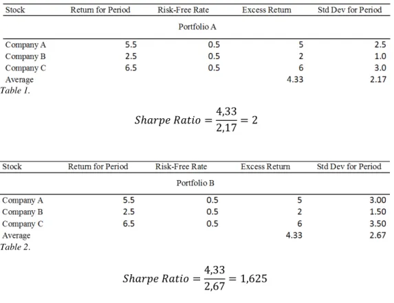
In the introduction the authors of this study briefly mentioned that diversification and risk is part of a larger context. All investments must ultimately be measured by their performance, in this case, by maximizing risk-adjusted return. The Sharpe ratio is introduced to measure the private Nordic investor’s individual economic welfare. In 1965, William F. Sharpe developed this measure that is now the industry standard for calculating risk-adjusted return. The Sharpe ratio is the average return over and above the risk-free rate, per unit of risk.

(14)

𝑆𝑆ℎ𝑉𝑉𝐶𝐶𝑎𝑎𝐶𝐶 𝑅𝑅𝑉𝑉𝐶𝐶𝑂𝑂𝑅𝑅 =𝑅𝑅�𝑝𝑝_𝜎𝜎− 𝑅𝑅𝑓𝑓 𝑝𝑝 𝑅𝑅�𝑝𝑝= 𝐴𝐴𝐴𝐴𝐶𝐶𝐶𝐶𝑉𝑉𝑂𝑂𝐶𝐶 𝑎𝑎𝑅𝑅𝐶𝐶𝐶𝐶𝑝𝑝𝑅𝑅𝑉𝑉𝑂𝑂𝑅𝑅 𝐶𝐶𝐶𝐶𝐶𝐶𝐶𝐶𝐶𝐶𝐶𝐶 𝑅𝑅𝑓𝑓 = 𝑅𝑅𝑂𝑂𝑅𝑅𝑅𝑅 𝑝𝑝𝐶𝐶𝐶𝐶𝐶𝐶 𝐶𝐶𝑉𝑉𝐶𝐶𝐶𝐶 𝜎𝜎𝑝𝑝= 𝑃𝑃𝑅𝑅𝐶𝐶𝐶𝐶𝑝𝑝𝑅𝑅𝑉𝑉𝑂𝑂𝑅𝑅 𝑅𝑅𝐶𝐶𝑉𝑉𝐶𝐶𝑠𝑠𝑉𝑉𝐶𝐶𝑠𝑠 𝑠𝑠𝐶𝐶𝐴𝐴𝑂𝑂𝑉𝑉𝐶𝐶𝑂𝑂𝑅𝑅𝐶𝐶 Equation 7.

The portfolio return (𝑅𝑅_𝑝𝑝) is calculated by using the monthly returns over the previous years, thus, the average portfolio return (𝑅𝑅�_𝑝𝑝) is the portfolio returns summed and divided by the number of return data points. The risk free rate (𝑅𝑅_𝑓𝑓) is the rate of return an investor would expect from an entirely risk-free investment. Nordnet uses a risk free rate deducted from the three-month Swedish Treasury bill to calculate the Sharpe ratio (www.nordnet.se, 2016). As mentioned, the variance is the standard deviation squared; therefore, in order to calculate the portfolio standard deviation (𝜎𝜎_𝑝𝑝) one calculates the square root of the portfolio variance (�𝜎𝜎_𝑝𝑝2=𝜎𝜎_𝑝𝑝) (Levy & Post, 2005). By subtracting the risk-free rate from the average return, one can isolate the return associated with risk-taking. In this formula, risk is simply measured as the portfolio standard deviation. This can be illustrated by an example: Consider two investors allocating their financial assets as in portfolio A (table 1) and B (table 2). The Sharpe ratio is determined by: 1) subtracting the risk-free rate of return from each investment return during a given period to get the excess return; 2) summarizing the average portfolio excess returns; and 3) dividing the portfolio excess returns with the average standard deviation of those same investments.

Table 1. 𝑆𝑆ℎ𝑉𝑉𝐶𝐶𝑎𝑎𝐶𝐶 𝑅𝑅𝑉𝑉𝐶𝐶𝑂𝑂𝑅𝑅 =4,33_{2,17 = 2} Table 2. 𝑆𝑆ℎ𝑉𝑉𝐶𝐶𝑎𝑎𝐶𝐶 𝑅𝑅𝑉𝑉𝐶𝐶𝑂𝑂𝑅𝑅 =4,33 2,67 = 1,625 14

(15)

Notice that although portfolio A and portfolio B share the same excess returns, they do not share the same Sharpe ratio. Portfolio A exhibits higher Sharpe ratio, and thus, benefits from a greater risk-adjusted return. This is because portfolio B is not appropriately compensated for the greater amount of risk it is exposed to, the higher standard deviation is not justified. The benefit of measuring the Sharpe ratio is the ability to compare investors with different risk and returns. Judging by portfolio B’s lower Sharpe ratio, one can immediately draw the conclusion that owner of portfolio B suffers from inefficiency and individual welfare loss.

2.6 CONNECTING THE DOTS

On account of diversification, it is paramount to manage the inherent risk of financial investing. To assess by what means one portfolio is diversified, the authors measure the total number of stocks and how the covariance between stocks affect the portfolio normalized variance. The potential welfare losses examined in this study are costs caused by the private Nordic investors’ suboptimal decision making, and to put diversification in relation to such welfare losses, this study utilizes the Sharpe ratio, which measures risk adjusted return.

(16)

3. Method

In this study, the authors limit the scope to diversification between equity investments, more specifically, direct ownership of stocks or, indirect ownership of stocks through equity funds. The authors of this study acknowledge that diversification is important to all investments, however, it is their opinion that diversification is mostly important when dealing with stocks. There are two reasons for this, firstly, equity investments are by nature generally more volatile than other investments, and hence, the urgency of diminishing risk is greater. There exist exceptions with high-yield bonds, options, futures or other advanced derivatives, but they are comparatively uncommon and rarely invested in by the general public. The second reason is that stocks are, in contrast to other derivatives, commonly owned by the public, making it relevant for most people. In addition to this, the absolute majority of studies made over the last century have been focused on equity investments, although the reason for this is unknown (Elton & Gruber, 1977, Statman, 1987, Brennan & Torous, 1999, Goetzmann & Kumar, 2008).

The scope of this paper is restricted to private Nordic investors. Nordic investors imply citizens of Sweden, Norway, Denmark and Finland. Private investors refer to individuals within these countries without any known connection or support by professionals or institutions. The reason for including details about each individual country was solely due to the fact that making generalizations about the entire Nordic area would only have given a limited understanding of the reality. The intention was not to compare and discuss differences between the countries and why such differences exist.

3.1 DATA

The data was collected from Shareville, a database provided by Nordnet Bank AB (henceforth referred to as the database), containing present and historical data on 80,000 private Nordic investor’s and their investments. In method, Nordic private investors are henceforth referred to as users. Each user in the database have initially been created with a social security number, validating the individual’s legitimacy and uniqueness. The data on each user’s individual holding is provided by NASDAQ, intermediately through Nordnet. Because Nordnet, unlike traditional banks, do not provide guidance in investment choices to their users, the authors of this paper believe that the bank’s user base serves as an accurate representation of the investor’s ability to diversify. The usage of data gathered from a traditional bank is likely to produce unreliable estimations, as the investor’s investment choices becomes influenced by a guiding advisor. This is the reason why Nordnet’s database was used in this study. Furthermore, considering that the collection was made from a single database where all the information is computed similarly, this study benefits from uniformity and risk of sample errors is mitigated.

Because Shareville is not a database designed for statistical purposes, the data the authors took part of was in such a specific and rudimentary form that the authors had to construct a program to sort and analyze the data. There was no data handling program available to the authors that met the requirements to carry out the demanded tasks. To give a conceptual idea of the sampling procedure, a simplified, non-technical explanation of how the process would have been executed without a

(17)

computer program follows. The first text file contains 80,000 rows, each corresponding to a user with the following information: user ID, the user's nationality and her Sharpe ratio. These 80,000 users are divided into four pools, divided by nationality. From each pool, 4000 samples are randomly selected, making up four sample pools, one for each country. At this stage, a sample pool of user profiles exists, however, with incomplete user profiles, as they miss information about their holdings. The second text file holds 336,000 rows of information, each row representing a security, identified by a security ID connected to the user profile it belongs to and the weight the security has in the user's portfolio. For each sampled user in the four pools previously composed, a portfolio is constructed by matching the user ID in the sample pool against user IDs in text file B. At this stage, all user profiles have a user ID, nationality and a portfolio containing securities with their corresponding portfolio weight. Finally, the third text file holds 9000 rows, each row providing a security ID and the actual name of that security. By matching each users' portfolio, currently only containing security IDs, with the securities' actual name from text file C, one arrive at a comprehensive sample base. As this process is finished, 4000 users can now be identified by their user IDs, nationalities, Sharpe ratios and portfolios with the securities' actual name and weight included. This sample base was used to compute and compose the tables and figures provided in Appendix B. The process of sampling and computing a comprehensive statistical data set is simple conceptually, but time consuming to manage manually. To facilitate this process, and to minimize sampling errors, two computer programs was designed by the authors to carry out the tasks automatically. The remaining risk of errors from programming mistakes was diminished by reviewing the programs thoroughly with the aid of Niil Öhlin, a professional programmer from Atea Group, to guarantee that the sampling and computations are handled correctly. The technical description of the two programs is explained below and their details are provided in the Programs section in Appendix B.

The data provided consisted of three files (comma separated values files). CSV-files are simple text documents, structured with one data point per line. The first file contained information about each individual's ID, nationality and Sharpe ratio. The second file provided each user's investments by ID and its weight in the user's portfolio. Lastly, the third file held the security ID and their actual corresponding name. Two separate programs managed the data consecutively. Firstly, Program 1 (code page 1) loaded the CSV-files and sampled 4000 users from each nation. In the sampling process, each sampled user was validated by making sure that the user’s data was free from evident errors, meaning that the user’s info contained all necessary data and that the user had a Sharpe ratio within reasonable boundaries (± 10). Each sample was then compiled to four new files, one for each nation. Program 2 (see code page 2) loaded the new files and sorted all information (see code page 4) to construct a final data type (see code page 11) for each user containing the following information: user ID, user nationality, user Sharpe ratio and user portfolio including security names and weighting. Such a data type, holding the user's information was created to minimize the risk of losing or interweaving data between users. An important detail in the sorting process is that Program 2 sorted securities into two categories, stocks and other securities. Thereafter, a similar data type (see code page 12) was created for each country to hold the outputs from the later conducted

(18)

calculations. This data type was also created to minimize the risk of losing or interweaving data, but between countries. The following calculations (see code page 5 for execution & code page 7 for definitions) were made for each country and stored in the new data type: average number of stocks, average number of other securities, Sharpe ratios sorted by average number of stocks, average country wide Sharpe and the country's average portfolio. The final step of Program 2 was writing all the outputs of the calculations described above to file (see code page 6), making it available to the authors of this paper. The file format used as output was, again the CSV-file format. The average portfolio was generated with aid of Program 2. The program ordered the 10 most commonly owned securities for each country with their corresponding weighting, the average portfolio was then constructed manually by adding the number of average securities of that asset class and their weighting to the portfolio. Because the weightings are measured as the average weighting of such an investment, they do not add up to a 100%, hence, the authors rescaled the weighting scheme proportionally to each original weight. The calculation can be illustrated with an example:

Table 3.

Sweden has following data: Average number of stocks: 4

Average number of other securities: 2

The most common stock, ordered by number of occurrences in user portfolio, and weighting in rounded percentages:

The authors use the number of occurrences to pick out the top 4 stocks and top 2 other securities from the 10 most common securities. Hence, after proportional weighting we get this structure.1

1_{In this example only rounded percentages are shown, due to a better overview.}

18

(19)

Table 4.

The sample size used of 4000 was determined by three factors described in the article of Israel (1992); the level of precision, the confidence level, and the degree of variability. The level of precision indicates how well the sample is reflecting the true value of the population (ibid). In this study the authors wanted to be as precise as possible when determining the average investor, therefore the decision was made to have a level of precision of at least (± 3%), meaning that if one conclude that 90% of the Nordic investors have more than 50 stocks in their portfolio, the reader can assure that it is true between 87% and 93% of the Nordic investors. The confidence level have a similar purpose, it indicates to which degree one can find the true value of the population when repeating the same sample size. The authors of this study use a sample size with a confidence level of 95%. Another important factor when deciding the sample size is the degree of variability. Depending on whether the population is homogenous or heterogeneous, meaning, if the attributes of the population are similar or different to each other, have an effect on the sample size needed. If the attributes are atypical, a larger sample size is needed to estimate the true value of the population than if they were similar (ibid). The highest degree of variability is 50%, since a higher or lower degree of variability indicate that “a large majority do not or do, respectively, have the attribute of interest” (ibid). Thus, for this study the authors use a degree of variability of 50% since the Nordic investors’ portfolios have varying compositions. In the study of Israel (1992), he provide indications that with a population of 100,000, which is significantly larger than our data base, with a (± 3%) level of precision, 95% confidence interval, and a 50% degree of variability one should utilize a sample size of 1099. However, the authors of this study increased the sample size until the point it became impractical for the program to collect the data. This provides evidence that the sample size of 16,000 users is more than enough to be statistically reliable for the 80,000 users.

3.2 MANAGING THE DATA

The authors weighed and calculated the percentages of occurrences of every security for each average portfolio, as the first step of determining the variables of the average portfolios. The authors are utilizing the formulas given in the book of Levy and Post (2005) for estimating the security standard deviation, variance, and covariance between securities, the portfolio variance and the correlation between securities and rate of return. The authors of this study find the book of Levy and Post (2005) to be a reliable source because it is peer previewed textbook published by the well-known Prentice Hall, a major educational publisher. The NV measure, however, is reused from the peer-previewed study of Goetzmann and Kumar (2008). To calculate the

(20)

standard deviation and variance of each security, the authors of this paper downloaded separate spreadsheets of historical prices for each security from Yahoo Finance (www.finance.yahoo.com, 2016). However, since Yahoo Finance only covers data on stocks and not other types of securities, such as funds, the authors had to register the monthly prices manually by looking at the price of each fund, at the beginning of every month, on Nordnet’s database website (www.shareville.se, 2016). To gather the prices from www.shareville.se the authors scanned the graph of each fund manually as there were no lists of data provided. The authors used monthly prices over a period between June of 2014 and May of 2016. The reason from the starting point June of 2014 is because three of the most commonly owned funds of the average investor came to the market at that time (Nordnet Superfondet Norge, Nordnet Superrahasto Suomi, and Nordnet Superfonden Danmark). The authors of this paper believe that a two-year period is sufficient for determining the correlation between the securities. The prices were converted into dollars, for the purpose of having the same currency for every security, and structured in Excel tables for each security.2_{Furthermore, by utilizing the prices, the authors calculated the rate of return} for each month using the formula in equation 3 into an additional table. With the rates of return the authors calculated the variance-covariance matrix and the correlation matrix. Starting with the variance-covariance matrix, as explained in the section of portfolio variance the matrix consists of the covariance of each element multiplied with each other, where the covariance multiplied with itself results in the variance of that security (Levy & Post, 2005). To determine the variance-covariance matrix presented below, the authors started to calculate an excess return table by subtracting the return by the mean return of each security. Further, the authors multiplied the excess return table by itself transposed by using matrix multiplication in Excel, then divided the matrix by the number of observations in the dataset, which in our case was 22 for the rates of return collected.

Panel L: The table gives the variance of each security labeled on the left hand side, and the covariance between them.

2_{The exchange rates were collected May 2, 2016. USD/NOK=8.0532, USD/SEK=8.0357,}

USD/DKK=6.5003, EUR/USD=1.1449 (www.nordnet.se, 2016).

20

(21)

In the variance-covariance matrix, each security on the left-hand side is connected to one number, to mitigate the navigation of the matrix. The table shows the variance of each security along the gray diagonal and the covariance between each security in the other spaces. The variance is the standard deviation squared by the same value, where the standard deviation is measured in percentages. However, the variance in the matrix can be misleading since we are calculating with decimal numbers. Thus, the variance of for example fundamental stock pick looks like it is 0,22% when it is 22%. This does not affect the calculations of the NV since every step is determined in the same way. Each variance was transferred into the average portfolios. The variance-covariance matrix does not provide any valuable information about the strength of the correlations; therefore, the authors calculated a correlation matrix shown below. The correlation matrix is calculated as follows. First, the authors calculated a matrix of the standard deviation in the same way as when calculating the variance-covariance matrix. Then, by dividing the variance-covariance matrix by the standard deviation matrix, it results in this correlation matrix.

Panel K: The table gives the correlation between each of the 25 securities labeled on to the left hand side.

The table is structured the same way as the variance-covariance matrix, with the numbered securities to the left. By looking at the correlation matrix, the authors can see that it has a gray diagonal of 25 1s, implying that the correlation between every security and itself equals 1. Thus, it gives us indications that the calculations have been done correctly. To measure the portfolio variance for each average portfolio the authors utilized the formula in equation 6. In this formula, we use the weighing which the authors calculated in the beginning, together with the variances and covariances of each security from the matrices. To be consistent with the average portfolios securities, the authors calculated the standard deviation of each portfolio, to include in the variable table, by taking the square root of the portfolio variance. Subsequently, to determine the NV for every average portfolio the authors divided the portfolio variance of every portfolio by the mean variance of every security in each portfolio. All variables described in this section are included in the table below:

(22)

Panel J: The table gives the standard deviation, portfolio variance, mean variance of stocks, average correlation, the normalized portfolio variance and the Sharpe ratio of Denmark, Finland, Norway and Sweden.

3.3 ETHICS

Ethical issues must be taken into consideration when dealing with information about the private Nordic investors. Even though each profile is connected to a social security number, the authors of this paper do not have access to such information. Furthermore, the user-ids of the 80,000 investors only comprises of information about the investor holdings, and there is no information that can be regarded as sensitive or sufficient enough to trace it back to the investor.

3.4 LIMITATIONS

Given that Program 2 is somewhat complex, the authors of this paper cannot exclude the possibility of programming errors. However, after the program was constructed, the program was reviewed three times by the authors and, in addition, by a professional programmer from the IT-infrastructure developing company Atea Group, Niil Öhlin. Taking everything into consideration, the authors of this paper deem the probability of programming errors to be very small. Although data errors were mitigated in the sampling process, it is difficult to verify that all data received by Shareville was free of errors. The authors of this paper did, however, authenticate the data by verifying 10 user-IDs against the available database provided on Shareville’s website. In the unlikely event of data errors and abnormalities (e.g. abnormal returns), as previously mentioned, safeguards were put into the program, to exclude sample data errors.

(23)

4. Results and Discussion

4.1 THE AVERAGE PORTFOLIOS

The average portfolio component is a necessity for the authors to make assumptions about the Nordic investor, the average investor portfolios are provided in panel F through I below.

Panel F: The table gives the average portfolio of Sweden. It show us the portfolio’s average weighting, the standard deviation, the variance and the occurrence ratio. The occurrence ratio is the number of times the security was detected in a sampled portfolio as a percentage of the whole sample size.

Firstly, noteworthy is the fact that all four investors seem to favor domestic equities or, at least, equities originating from the Nordic regions. Looking at the Swedish portfolio in Panel F, the companies Hennes & Mauritz, TeliaSonera, Betsson and Investor are all wholly or partly Swedish. Nordnet Superfonden Sverige is a passive index fund constructed to follow the Swedish OMXS30 index. The company with the highest weight within the fund is Hennes & Mauritz (www.nordnet.se, 2016). Spiltan Aktiefond Investmentbolag is a fund composed of several Swedish investment companies including: Industrivärlden, Investor and Kinnevik, ordered by greatest weight first (ibid). This portfolio includes one comparatively volatile asset, as the standard deviation indicates, which is the Swedish company Betsson, providing services for online gaming (www.betsson.com, 2016).

Panel G: The table gives the average portfolio of Norway. It show us the portfolio’s average weighting, the standard deviation, the variance and the occurrence ratio. The occurrence ratio is the number of times the security was detected in a sampled portfolio as a percentage of the whole sample size.

The average Norwegian portfolio in Panel G appears to only include one stock. The Norwegian average portfolio is also evidently favoring Nordic companies, with the volatile Norwegian Air Shuttle as their most popular stock. Also, three out of four funds contains stocks from either the Norwegian or Nordic market. However, it is the only portfolio including a fund with International geographical exposure, DNB Global Indeks. DNB Global Indeks is a passively managed index fund following the MSCI World Index with greatest weighting in North America (www.nordnet.se, 2016).

(24)

Panel H: The table give the average portfolio of Denmark. The table gives us the portfolio’s average weighting, the standard deviation, the variance and the occurrence ratio. The occurrence ratio is the number of times the security was detected in a sampled portfolio as a percentage of the whole sample size.

Denmark's portfolio in Panel H includes three comparatively riskier investments, the first one being Fingerprint, the only growth company among the portfolios. It is surprising that substantial allocation is put in this stock, considering its comparatively high volatility, indicated by its variance. The second is Genmab, a Danish biotechnological company with a variance of 105.68. The third volatile investment is Danske Invest Bioteknologi, being an equity fund, containing biotechnological corporations.

Panel I: The table gives the average portfolio of Finland. It shows us the portfolio’s average weighting, the standard deviation, the variance and the occurrence ratio. The occurrence ratio is the number of times the security was detected in a sampled portfolio as a percentage of the whole sample size.

The Finnish portfolio in Panel I do not seem to diverge from the other portfolios significantly other than being slightly more diversified outside the domestic boundaries but inside the Nordic region. It is also noteworthy that the portfolio allocates the preponderant weighting (27%) to one company, Telia Sonera, a company owned partly by the Swedish and Finnish governments (www.teliacompany.com, 2016).

Aggregated, it is apparent that the general Nordic investor commonly owns stable corporations with high market capitalization (total market value) and high dividend yields, indicating a low-risk profile in the equity segment. Each portfolio tends to include at least one security, which is more volatile than the average, except for the Finnish average portfolio, with no particular outliers. The stocks generally exhibit low price variances with the exception of Fingerprint, with the variance of 728,46. Assuming that the Nordic investor has a fundamental understanding of diversification, meaning that she understands that buying different stocks is beneficial for her portfolio. Then, looking at the Nordic investor's combinations of stocks and

(25)

funds, one could suspect that she is unintentionally overexposed to certain stocks indirectly. For instance, the Swedish investor holds substantial amounts of direct ownership in Hennes & Mauritz (H&M) while simultaneously holding additional indirect ownership in H&M, given that the fund Nordnet Superfonden Sverige includes H&M as its largest building block. The Swedish investor also directly owns Investor AB while simultaneously indirectly owning the same company through Spiltan Aktiefond Investmentbolag. Similar patterns can be detected in the Finnish investor's profile with KONE, Sampo and Nokia, all included in the fund Nordnet Superrahasto Suomi. Whether this level of holding is unwanted or not is difficult to say with current data, but the consequences may be overexposure to unsystematic risk from those specific companies. More importantly, it is likely to increase correlations between holdings that may, in extension, incur welfare losses. However, because the average portfolios rely on averages, it is also possible that the portfolios reflects several investors, which have no simultaneous ownership of one stock, although, the authors deem this possibility to be unlikely.

4.2 DIRECT OWNERSHIP

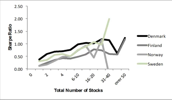
It seems that later studies argue that investors need increasingly more stocks in order to be diversified. In this paper, discoveries made in the latest study about the total number of stocks (Benjelloun, 2010) will be adopted and the diversified portfolio will be defined by Benjelloun’s threshold of 40-50 stocks, solely looking at total number of stocks. To make conclusions on the Nordic investor’s diversification by the total number of stocks we regard their average holdings below.

Panel E: The table gives the average number of stocks and the average number of other securities of Finland, Norway and Sweden.

Firstly, our results in panel E reveals that none of the countries have an average number of stocks higher than 6, and by calculating the countries’ average of averages, one can compute that the mean number of stocks for the Nordic investor is 4. Considering that Benjelloun (2010) showed evidence that the total number of stocks required to stretch between 40 and 50, it seems apparent, only looking at the total amount of stocks, that the Nordic investor is under-diversified. Although Benjelloun (2010) has provided the most recent study of this, previous studies have indicated otherwise. Elton and Gruber’s study in 1987 suggested that the marginal benefit of increasing the total number of stocks is only significant up to a total of 10 stocks, however, none of the Nordic countries’ averages meet that threshold either. Regardless if one uses the thresholds presented in this paper or other conventional thresholds in older diversification literature, the results still seem to indicate under-diversification. At a glance, the reader might be questioning the high percentage of investors holding zero stocks in their portfolio (see Appendix for Panel A showing investor’s average stock holdings). Indeed, it seems questionable that 63 % of Norwegians have no holdings at all, but this result does not show the whole picture,

(26)

only direct ownership. It is reasonable to say that a significant part of the investors’ stocks are held through indirect ownership.

4.3 INDIRECT OWNERSHIP

Despite that the average investor appears to be under-diversified purely by looking at direct ownership of stocks, each of the countries have an average number of other securities of least 2, presented in Panel E. This indicates that each individual may, in fact, be diversified indirectly if such a security turns out to be an equity fund, containing multiple of other stocks. Based on previous assumptions laid out about the average portfolios, the authors can conclude that it is, indeed, likely that the other security turns out to be an equity fund. By investigating the mutual investments between the average portfolios one can draw the conclusion that Nordnet’s equity funds (Nordnet Superfonden Sverige, Nordnet Superfondet Norge, Nordnet Superfonden Danmark, and Nordnet Superrahasto Suomi) are the most common funds. Nordnet Superfonden Danmark contains, among mentioned funds, the least amount of stocks, totaling 20 stocks (www.morningstar.se, 2016). With that said, it is reasonable to say that even though, the average Nordic investor would hold no stocks through direct ownership, she would hold at least 20 stocks in indirect ownerships through funds. In conclusion, looking at the other countries and their combined averages of 2, the average Nordic investor would be diversified with over 40 stocks by indirect ownership through funds, making her in this regard, diversified. Furthermore, there are significant percentages (5-17%) in the upper spans of 6-10 holdings of other securities in Panel B below. Hence, based on the previous assumption, that equity funds hold at least 20 stocks, a sizeable amount of investors seem to be in indirect ownership of 120 to 200 stocks. If this were true, such a Nordic investor would reach and exceed the total number of stocks threshold of 40-50 stocks, by a substantial margin.

Panel B: The table gives the average percentages of portfolios for Denmark, Finland, Norway and Sweden, ordered by the average total number of other securities.

There are a number of reasons why this paper utilizes Benjelloun’s assumptions about the diversification thresholds. The measuring of diversification is not new science; Benjelloun’s methods are built on previous research (Evans & Archer, 1968, Elton & Gruber, 1977, Campbell, Lettau, Malkiel and Xu, 2001) that has been iterated upon over the last 50 years. The authors regard Benjelloun’s methods to be the most

(27)

contemporary, as it takes into consideration the latest research and the modern structure of the financial system. Furthermore, Benjelloun's study provides the most complete picture by examining the size of a well-diversified portfolio using both equal and market weights.

4.4 THE NORMALIZED VARIANCE

In panel J, the authors have summarized the relevant variables of diversification and performance to evaluate the average portfolios. The table presents, from the top to bottom: the portfolio standard deviation calculated using historical prices converted into percentage rates of return, the portfolio variance which is the portfolio standard deviation squared, mean variance of securities for each portfolio, the average correlation between securities for each portfolio, the normalized variance (NV), and the Sharpe ratios. The standard deviation is part of the formula for calculating the Sharpe ratio. However, the authors had the Sharpe ratios provided by Nordnet and was therefore not calculated. The normalized portfolio variance was calculated by dividing the portfolio variance with the mean variance of securities.

Panel J: The table gives the standard deviation, portfolio variance, mean variance of stocks, average correlation, the normalized portfolio variance and the Sharpe ratio of Denmark, Finland, Norway and Sweden.

In the study of Goetzmann and Kumar (2008) they showed that by increasing total number of stocks while maintaining low correlations, the NV measure decreases with a greater diversified portfolio. Their data provided evidence that a diversified portfolio range between an NV value of 0.163 and 0.407, where the lower value indicate a well-diversified portfolio and the higher value a moderately diversified portfolio; in this study, these thresholds are utilized to make conclusions about whether the Nordic investor is diversified. Overall, all Nordic countries have scores which all lies within the threshold of Goetzmann & Kumar (2008). Most of the Nordic countries are on the upper span, except Sweden, with slightly lower NV of 0.26. By looking at the mean variance of securities, the conclusion can be made that Nordic countries are withholding a different amount of risk in their portfolios; Denmark clearly has the portfolio with the highest risk, showing a mean variance of 156,7. As shown in the average portfolio of Denmark in Panel F, the portfolio includes the highly volatile stock Fingerprint, exhibiting a large standard deviation, which is increasing the inherent risk of the whole portfolio. Finland seems to have a less risk-exposed portfolio, because of the relatively stable holdings as shown in Panel G. Sweden and Norway, on the other hand, lies somewhere in between with one volatile stock each, Betsson AB and Norwegian Air Shuttle AS respectively. If considering again the normalized variance, the country with the lowest mean variance of securities also have the lowest NV value; however, the highest mean variance of

(28)

securities doesn’t have the highest NV value, which makes it questionable that the mean portfolio variance determines the whole picture of diversification. For example, regard the Norwegian portfolio. It has a considerably lower mean variance of securities than Denmark, while it has a higher NV value. To explain why the NV value and the mean variance of securities are incoherent, the correlation matrices must be analyzed.

Panel M: The table gives the correlation between each of the 5 securities in the Norwegian portfolio, labeled on to the left hand side.

The way the authors calculated the average correlation, which is stated in Panel J, is by adding all correlations on one of the sides of the diagonal and then dividing the sum by the number of data points. This was done to determine whether the portfolio holdings have an overall high or low correlation. The figure presents the correlation between the securities within the Norwegian portfolio. It appears to be that a significant part of the securities has a high correlation, which explains why the average Norwegian portfolio has a high NV value. The average correlation of holdings is 0.49 in the Norwegian portfolio. However, because the weighting of each security within the portfolio determines its impact, it is essential that it is taken into consideration. Although, the Norwegian portfolio have very even weighting on each security, making each security to have a similar impact. In contrast to the Norwegian portfolio’s average correlation level of 0.49, the average correlation between the securities in the Swedish portfolio is 0.25, which is significantly lower than the Norwegian portfolio. Furthermore, since the Swedish portfolio has an even weighting scheme, its average portfolio correlation should be an accurate depiction of its true average correlation. This Swedish portfolio’s correlations are shown in the matrix below.

Panel L: The table gives the correlation between each of the 6 securities in the Swedish portfolio, labeled on to the left hand side.

Although the average Swedish portfolio exhibits low average correlation, there appears to be two exceptions: Nordnet Superfonden Sverige and Spiltan Aktiefond Invest, together with Hennes & Mauritz AB and Investor AB. The two funds seem to

(29)

correlate almost perfectly along with the two stocks, as they also have high correlation. However, the NV value of the Swedish portfolio is considerably lower compared to the one of the Norwegian portfolio. It is likely that this is the result caused by a lower average portfolio correlation, diminishing the NV value significantly. The portfolio with the highest number securities is the Finnish average portfolio in the figure above.

Panel O: The table gives the correlation between each of the 9 securities in the Finnish portfolio, labeled on to the left hand side.

The portfolio has an average correlation value of 0.29, which is relatively higher than the Norwegian and Swedish portfolios. By looking at Panel I it is evident that there is great weight in Nordnet’s own funds. These are highly correlated, with a correlation value of 0.8 and 0.7, due to two reasons. Firstly, all three of the inherent Nordnet funds have a narrow geographic distribution, all stocks are domestic or from the Nordic region (www.morningstar.se, 2016). Secondly, the funds have great weight in financial and/or industrial industries (ibid). There are a variety of positively and negatively correlated securities with different amount of weight in the portfolio; Telia Sonera AB is the security that has the highest weight in the portfolio and high correlation with other securities. The highly correlated funds and the significant weight in the stock Telia Sonera AB, being highly correlated with Sampo and KONE, seem to have increased the NV value. In contrast to the previous portfolios, the average Danish portfolio’s NV value appears not to have a direct connection to the average correlation value. This can be seen below in Panel N below.

Panel N: The table gives the correlation between each of the 7 securities in the Danish portfolio, labeled on to the left hand side

The average Danish portfolio has a spread of negatively and positively correlated securities. Moreover, there is a high correlation between Danske Invest and Fundamental Invest, and also between, Genmab and Vestas. By comparing the

The Invisible Threat of Welfare Loss for Private Nordic Investors: A study on diversification