Mispricing Due to Nelson-Siegel-Svensson model

Mispricing

Due to Nelson-Siegel-Svensson model

Supervisors:

Author:

Senior Lecturer Jan Röman Neda Kazemie

jan.roman@mdh.se

kazemieneda@gmail.com

Examiner:

Professor Anatoliy Malyarenco Senior Lecturer Linus Carlsson

anatoliy.malyarenko@mdh.se

linus.carlsson@mdh.se

Acknowledgment

Foremost, I would like to express my deep gratitude to Senior Lecturer Jan Röman, for his advice,

encouragement, comments and invaluable help and guidance during the elaboration of this thesis. My

sincere thanks also go to Professor Anatoliy Malyarenko and Senior Lecturer Erik Darpö, for their

insightful comments and questions.

Last but not the least, I would like to express the deepest appreciation to my family and Morsal family for

their kind support during my study.

Abstract

Most trading software in the market uses linear interpolation in the bootstrap procedure to create a zero

coupon interest rate curve. Forward interest rate curves created by interpolation method have a zigzag

form that is inconsistent with arbitrage condition. Furthermore in the real world we are not able to detect

the spot rates for all periods because the number of traded instruments is limited.

Nelson and Siegel in 1987 proposed a model to estimate the interest rates. They demonstrated that their

model was flexible to capture the various possible shapes of the yield curve and estimates the term

structure of interest rates over time.

Many Central banks are using the extended Nelson-Siegel model (sometimes called the

Nelson-Siegel-Svensson model). This curve is parameterized with exponential functions, is smooth in both zero rate and

forward rate and overcome those barrier (data mining problems and zigzag shape of forward interest rate

curve), that we face by using linear interpolation to build the yield curve. The objective of this thesis is to

study the Nelson and Siegel model and its extended version by Svensson, furthermore, study the

adequacy and forecast performance of Nelson-Siegel-Svensson model in building the term structure of

interest rate comparing with the linear interpolation method.

2

Contents

1.3.2. Problem specification and discussion ... 7

1.3.3. Target Audience ... 7 ... 8 2.1. Interest Rates ... 8 2.1.1. Spot Rate ... 8 2.1.2. Discount function ... 8 2.1.3. Discount curve ... 9 2.1.4. Forward rate ... 10 2.1.5. Yield to maturity ... 11 2.1.6. Repo rate ... 11

2.2. Term structure of interest rate (Yield curve) ... 11

2.3. Par rate ... 12

2.3.1. Par rate for a bond ... 12

2.3.2. Par rate for a swap ... 12

2.4. Interbank rate ... 13 2.4.1. EURIBOR ... 13 2.4.2. EONIA ... 13 2.4.3. LIBOR ... 13 2.5. Instruments ... 14 2.5.1. Bonds ... 14 2.5.2. Swaps ... 14

2.5.3. Forward Rate Agreements (FRA) ... 15

2.5.4. Deposit (Certificate of Deposits)... 15

2.6. Bootstrapping interest rate curves ... 16

2.7. Interpolation ... 16

3

... 17

3.1. The Original Model ... 17

3.2. Deriving the equation for the forward rate by using the Nelson-Siegel model ... 18

3.3. The extended version of Svensson ... 21

3.4. Fixing the parameters of the model ... 23

... 24

4.1. Curve construction of interest rate ... 24

4.2. Bootstrapping ... 25

4.3. Linear Interpolation ... 27

4.3.1. Linear interpolation on discount factor ... 27

4.4. Interest Rate Swap valuation (traditional approach) ... 28

4.5. Financial crisis and its effect on pricing methodology ... 30

4.5.1. Market practices for pricing interest rate derivatives in multi-curve framework. ... 31

... 33

5.1. Data and Parameters ... 33

5.2. Building the spot rate and forward rate curves ... 33

5.2.1. Data ... 34

5.3. Fitted Curves ... 37

5.3.1. Yield Curves... 37

5.3.2. Forward Curves ... 38

5.3.3. Discount Curves ... 40

5.3.4. Instantaneous Forward and Spot Curves by Interpolation ... 41

5.3.5. Forward and Spot Curves by Nelson-Siegel-Svensson Model ... 42

5.4. Valuing interest rate swaps ... 46

5.4.1. Yield Curves... 50 5.4.2. Forward Curves ... 51 5.4.3 Discount Curves ... 52 ... 54 Conclusions ... 54 ... 56

Summary of reflection of objectives in the thesis ... 56

7.1 Objective 1 - Knowledge and understanding ... 56

7.2 Objective 2 – Methodological knowledge ... 56

7.3 Objective 3 – Critically and systematically integrate knowledge ... 56

4

7.5 Objective 5 – Present and discuss conclusions and knowledge ... 57

7.6 Objective 7 – Scientific, social and ethical aspects ... 57

References ... 58

Appendix 1 ... 59

Appendix 2 ... 64

List of Figures ... 71

5

Introduction

1.1. Background

Term structures of interest rates, also known as yield curves are a measure of the markets expectation of future interest rates, given the current market conditions. When the yield curves are known, they are used to calculate present values of expected future cash-flows from financial contracts. To estimate an accurate term structure of interest rates is therefore one of the most important and challenging subjects in financial area. Without the yield curves we are not able to value financial instrument such as cash-flow instruments, equities, commodities and derivatives. Derivatives are financial contracts where the values are derived from expected future values of some underlying instrument.

Due to the importance of this issue, many researchers have developed methods and models to construct and forecast yield curves from prices of traded assets1_{. Most trading software in the market uses linear interpolation in}

a bootstrap procedure to create the term structure of interest rate. Such yield curves used for discounting goes under the name zero-coupon curves (or just zero-curves) or discount curves. Yield-curves representing the interest rate between two dates in the future are called term structure of forward rates. A large number of yield curves exists since they can be derived from different markets like the market of government bonds and the inter-bank market.

The forward rates can be calculated, via no arbitrage conditions via the zero rates. Here the market practice has been to use linear interpolation on zero rates. Forward interest rate curves created by a linear interpolation method have a zigzag form that is inconsistent with no arbitrage condition; moreover, illiquidity and missing data points are two main obstacles in bootstrapping methods. Therefore, other methods have been used to overcome these drawbacks.

One of the satisfactory models that provides smooth forward interest rate curve is the Nelson and Siegel model. This model was proposed by Nelson and Siegel in 1987 to estimate the interest rates. They demonstrated that their model is flexible to capture the various possible shapes of the yield curve and can estimate the term structure of interest rates over time. The model is parameterized with exponential functions and provides smooth yield and forward rate curves. This model was extended by Svensson in 1994 when he added a term allowing an extra bump in the yield curve.

According to Bank for International Settlements (BIS) 2005, central banks in Belgium, Finland, France, Germany, Italy, Norway, Spain and Switzerland have used the Nelson-Siegel model or one of its modifications as a method to estimate their term structure of interest rates.

1 _{See Nelson, Charles R. and Andrew F.Siegel.1987, Fabozzi, F. J., L. Martellini, and P. Priaulet. 2005, Diebold Francis X. and Canlin Li.} 2006, Hagan, Patrick S. and Graeme West. 2006.

6

1.2. Literature review

The original model of Nelson-Siegel and its extended versions have been the subject of many academic researches and studies since the first introduction in 1987. These researches provide evidence that the model is capable of successfully and accurately building the term structure of interest rate and outperform the competitive models, especially for longer forecast horizons, see Diebold and Li (2006), or Fabozzi, Martellini, and Priaulet (2005). Dullmann and Uhrig‐Homburg (2000) use the Nelson‐Siegel model to build yield curves of Deutsche Mark‐ denominated bonds and calculate the risk structure of interest rates.

According to Hodges and Parekh (2006) and Barrett, Gosnell and Heuson (1995) the Nelson and Siegel model is used by Fixed‐income portfolio managers to hedge their portfolios. Martellini and Meyfredi (2007) estimate the value‐at‐risk for fixed‐income portfolios by using Nelson-Siegel model.

1.3. Structure

1.3.1. Purpose

The focus of this thesis is on the extended version of Nelson-Siegel model (sometimes called the Nelson-Siegel-Svensson model). I use the Nelson-Siegel-Nelson-Siegel-Svensson model to build the term structure of interest rate and apply the term structure that is built by this model to study the mispricing2 _{in different financial instruments. I also use linear}

interpolation to build the term structure of interest rate, and I compare these two methods to see if prices, when using the extended Nelson-Siegel model, are close to the prices generated by interpolation method and market prices. The market instruments used in this thesis consists of Deposits, FRA (Forward Rate Agreements) and Interest Rate Swaps (IRS).

My study confirms the ability of the Nelson-Seigel-Svensson model to capture the various shapes of spot curves. This model provides smooth term structures in both zero rates and forward rates, therefore, provides better estimation to value instruments that have cash-flows on other days than the market data.

Prices obtained by the Nelson-Seigel-Svensson model are close to the market prices and prices generated by the interpolation method. Moreover, this framework avoids data mining problems which we face in bootstrapping and linear interpolation methods and provides accurate estimation for missing data.

2 _{The mispricing is defined as the difference between real market prices and prices given by using the Nelson-Siegel-Svensson curve in} discounting and/or to generate the cash-flows in the instrument contracts.

7

1.3.2. Problem specification and discussion

Forward interest rate curves created by the interpolation method have a zigzag form that is inconsistent with arbitrage condition. Moreover, illiquidity and missing data points are two main obstacles in bootstrapping methods. I will examine Nelson-Siegel-Svensson model to see if the term structure and forward rate curve built by this model are accurate and smooth, compared with the curves that are built by the linear interpolation method. If it is the case, we can conclude that using the Nelson-Siegel-Svensson model is a better approach in building the term structure of the interest rate, since this model is parsimonious3_{, avoids data mining problems and provides smooth}

and accurate term structure of interest rate and forward curve.

1.3.3. Target Audience

Target audience for this thesis are students of financial mathematics and financial Engineering on advanced level. Good knowledge in mathematics and finance is assumed.

The remainder of this thesis is organized as follows:

reviews some definitions that are usedin this thesis.

introduces Nelson-Siegel model in its original form and extended version by Svensson.

is devoted to the methodology I have used to construct the term structure of interest rate and in both pre-and post-crisis market practices for valuing pre-and pricing interest rate swaps.

presents the data and empirical analysis and summarizes main points and concludes.

3 _{A model with few parameters}

8

Terminology

This Chapter presents some introduction into basic concepts which are mainly addressed in this thesis.4

2.1. Interest Rates

An interest rate is a rate a borrower pays to a lender for the use of money, it is usually expressed as annual percentage of the loan. Some of the different interest rates at the market which are used in this thesis are explained in the following Sections.

2.1.1. Spot Rate

The spot rate or short rate is defined as the theoretical profit given by a zero coupon bond. We use this rate when we calculate the amount we will get at time 𝑡1(in the future) if we invest X today. (I.e. at time 𝑡0)

𝑋𝑡₁= (1 + 𝑟(𝑡0, 𝑡1))𝑡1 𝑋𝑡₀

𝑃𝑉(𝑋𝑡1) =

1

(1 + 𝑟(𝑡0, 𝑡1))𝑡1

𝑋𝑡1 .

where 𝑃𝑉(𝑋𝑡) is the present value of 𝑋𝑡 and 𝑟(𝑡0, 𝑡1) is the spot rate.

In most cases, 𝑡0 is the current time (𝑡0= 0) and is sometimes dropped from notional convenience.

2.1.2. Discount function

The discount function 𝑝(𝑡0, 𝑡) describes the present value at time 𝑡0 of a unit cash flow at time t. This is a

fundamental function.

The remaining variable t refers to the time between 𝑡0 and t. The discount function is used as the base for all other

interest rates. These functions also represent the value of a zero-coupon bond at time 𝑡0 with maturity t.

At maturity a zero-coupon bond pays 1 cash unit ($, EUR, SEK etc.). Therefor 𝑝(𝑡, 𝑡) = 1.

One can prove the relationship between the spot rate and discount function as

𝑝(𝑡) ≡ 𝑝(0, 𝑡) = 1 (1 + 𝑟(𝑡))𝑡

4_{The information provided in this Chapter is mainly taken from John C.Hull, Options, Futures, and other Derivatives, 7}th _{ed., Prentice Hall}

9 Definition: Simple spot rate for period [𝑆, 𝑇] is defined by

𝑟𝑠𝑖𝑚𝑝(𝑆, 𝑇) = −

𝑝(𝑆, 𝑇) − 𝑝(𝑆, 𝑆) (𝑇 − 𝑆) 𝑝(𝑆, 𝑇) = −

𝑝(𝑆, 𝑇) − 1 (𝑇 − 𝑆)𝑝(𝑆, 𝑇)

Definition: Continuously compounded spot rate for period [𝑆, 𝑇] is defined by

𝑟𝑐𝑜𝑚𝑝(𝑆, 𝑇) = − ln(𝑝(𝑆, 𝑇)) − ln(𝑝(𝑆, 𝑆)) (𝑇 − 𝑆) = − ln(𝑝(𝑆, 𝑇)) (𝑇 − 𝑆)

2.1.3. Discount curve

The plot of the discount factor against time is known as the discount curve. The discount curve is monotonically decreasing and it never reaches zero since all cash flows no matter how far in the future they are paid are always worth more than nothing.

Figure 2.1: Discount Curve when rate =15%

0 0.2 0.4 0.6 0.8 1 0 2 4 6 8 10 12 14 D isc o u n t Fac to r Years

10

2.1.4. Forward rate

The concept of forward rate is closely related to a forward contract5. To define the today price for buying a zero-coupon bond at time 𝑡1 with maturity 𝑡2, 𝑡1< 𝑡2, we should set the future spot rate r for the period [𝑡1, 𝑡2]. This

future spot rate is called forward rate.

The relationship between forward rate and spot rate is given by

(1 + 𝑟(𝑡1)𝑠𝑝𝑜𝑡)𝑡1(1 + 𝑅(𝑡2− 𝑡1)𝑓𝑜𝑟𝑤𝑎𝑟𝑑) 𝑡2−𝑡1 = (1 + 𝑟(𝑡2)𝑠𝑝𝑜𝑡)𝑡2⇒ 𝑅(𝑡2− 𝑡1)𝑓𝑜𝑟𝑤𝑎𝑟𝑑 = ( (1 + 𝑟(𝑡₂)𝑠𝑝𝑜𝑡₎𝑡₂ (1 + 𝑟(𝑡₁)𝑠𝑝𝑜𝑡₎𝑡1) 1 𝑡2−𝑡1 − 1

Definition: Simple forward rate for the period [𝑡1, 𝑡2] contracted at time t

𝑅𝑠𝑖𝑚𝑝(𝑡, 𝑡1, 𝑡2) = −

𝑝(𝑡, 𝑡2) − 𝑝(𝑡, 𝑡1)

(𝑡₂− 𝑡1). 𝑝(𝑡, 𝑡2)

Definition: Continuously compounded forward rate for the period [𝑡1, 𝑡2] contracted at t

𝑅𝑐𝑜𝑚𝑝(𝑡, 𝑡1, 𝑡2) = −

ln (𝑝(𝑡, 𝑡2) − ln (𝑝(𝑡, 𝑡1)

(𝑡₂− 𝑡1)

Definition: Instantaneous forward rate

The instantaneous forward rate with maturity at T starting at 𝑡1, contracted at t is defined as

𝑅(𝑡, 𝑇) = lim 𝑡1→𝑇 𝑅(𝑡, 𝑡1, 𝑇) = − 𝜕ln (𝑝(𝑡, 𝑇)) 𝜕𝑇 where 𝑡 < 𝑡1< 𝑇.

11

2.1.5. Yield to maturity

Yield to maturity (YTM), also called Redemption Yield, is the interest an investor gains by holding an interest paying security until maturity, the investor is supposed to reinvest all coupon payments at the same interest rate during the lifetime of the security.

2.1.6. Repo rate

Sometimes trading activities are funded with a repo or repurchase agreement. This is a contract where an investment dealer who owns securities agrees to sell them to another company now and buy them back later at a slightly higher price. The other company is providing a loan to the investment dealer. The difference between the price at which the securities are sold and the price at which they are repurchased is the interest it earns. The interest rate is referred to as the repo rate.6 _{The periods in the repo market are usually:}

O/N (Over-Night), borrow and lending funds from today until tomorrow7. T/N (Tomorrow-Next), borrow and lending funds from tomorrow until next day.

C/W (Corporate-Week), borrow and lending funds from the day after tomorrow for a week.

S/N (Spot-Next), borrow and lending funds from the day after tomorrow until one business day ahead.

2.2. Term structure of interest rate (Yield curve)

The relationship between yield to maturity and time is called the term structure of interest rates. The visual representation of interest rate against time is known as yield curve.

The yield curve gives an idea about the future direction of the interest rate, therefore, building models which explain the shape of the yield curve has always been a challenge for investors and academics.

6 _{Jan Hull 7th edition (2009), p75}

12

2.3. Par rate

Par rate is the coupon rate that values an instrument to its nominal value.

2.3.1. Par rate for a bond

For simplicity assume that the nominal value of the bond is 100

100 = ∑(𝑝(0, 𝑡

) 𝐶

) + (𝑝(0, 𝑡

). 100) ⇒

𝐶

=

100. (1 − 𝑝(0, 𝑡

))

∑

𝑝(0, 𝑡

)

.

2.3.2. Par rate for a swap

The part rate for a swap is calculated as

∑(𝑝(0, 𝑡

) 𝐶

) = ∑ 𝑝(0, 𝑡

) 𝑅(𝑡

− 𝑡

)

⇒

𝐶

=

∑

𝑝(0, 𝑡

)𝑅(𝑡

− 𝑡

)

∑

𝑝(0, 𝑡

)

.

where dotted lines represent the floating rate at each payment date and straight lines represent the swap’s par rate. 𝐶𝑝𝑎𝑟 𝐶𝑝𝑎𝑟 𝐶𝑝𝑎𝑟 𝐶𝑝𝑎𝑟 0 = 100 100 =

13

2.4. Interbank rate

The Interbank rate is an interest rate decided by a number of investment banks and is defined as an average rate paid for short term loans between banks. Some of the interbank rates are LIBOR-London Interbank Offer Rate, STIBOR- Stockholm Interbank Offer rate, etc.

2.4.1. EURIBOR

Euribor (Euro Interbank Offered Rate) is a benchmark giving an indication of the average rate at which banks lend unsecured funding in the euro interbank market for a given period.

It is the rate at which Euro interbank term deposits are offered by one prime bank to another within the EMU zone (Economic and Monetary Union in Europe). It is produced for one, two and three weeks and for twelve maturities from one to twelve months8.

2.4.2. EONIA

Eonia (Euro Over-Night Index Average) is the effective overnight reference rate for the Euro. It is computed as a weighted average of all overnight unsecured lending transactions in the interbank market, undertaken in the European Union and European Free Trade Association (EFTA) countries. Eonia is computed with the help of the European Central Bank. The banks contributing to Eonia are the same first class market standing banks as the Panel Banks quoting for Euribor9_.

2.4.3. LIBOR

LIBOR is calculated and published by Thomson Reuters on behalf of the British Bankers' Association (BBA) after 11:00 AM (and generally around 11:45 AM) each day (London time). It is a trimmed average of interbank deposit rates offered by designated contributor banks, for maturities ranging from overnight to one year. LIBOR is calculated for 6 currencies10_{. There are eight, twelve, sixteen or twenty contributor banks on each currency panel,}

and the reported interest is the mean of the 50% middle values (the interquartile mean). The rates are a benchmark rather than a tradable rate; the actual rate at which banks will lend to one another continues to vary throughout the day. LIBOR is often used as a rate of reference for pound sterling and other currencies.

8_{http://www.euribor-ebf.eu/euribor-org/about-euribor.html(1/3/14)} 9_{http://www.euribor-ebf.eu/euribor-eonia-org/about-eonia.html(1/3/14)}

10 _{Before May 2013 there were 11 currencies. The following currencies have been removed; NZD, DKK, SEK, AUD and CAD. At the same}

14

2.5. Instruments

2.5.1. Bonds

Bonds are fixed-income securities, the buyer of the bond pays a price of P to the issuer and in returns receives a series of cash flows in the future.

Zero coupon bond (Also called “zero” or “pure discount bond”)

Is a bond that only has a single payment of one unit of currency (also called principal or notional amount), at maturity.

Coupon bond

Is a bond in which the buyer receives a sequence of interest payments (coupons) in specific dates (coupon payment dates) in addition to the principal.

Coupons usually are paid semi-annually or annually.

2.5.2. Swaps

A swap is an agreement between two parties to exchange cash flows during a specific period in the future according to two different indices (typically a floating interest rate-usually a LIBOR rate cash flow against a fixed rate cash flows). Swap agreements are interesting for counterparties due to the comparative advantages they have on borrowing money in capital markets which both parties can benefit (for example when a company wants to transform a floating rate loan into a fixed-rate loan due to the beneficiary it has in paying the fixed-rate interest and vice versa).

Plain vanilla interest-rate swap

Plain vanilla interest-rate swap is an agreement such that one party pays interest at a fixed rate for receiving interest at a floating rate from the other party based on a specified face value. Face value, payment frequency, time to maturity, day count convention, fixed rate and the floating rate must be defined in the contract.

15

Overnight indexed Swap (OIS)

With an overnight indexed swap, two parties agree that party1 receives a fixed rate from party 2 (the fixed leg of the swap), and party 2, receives a rate equal to the average of overnight rate from party1 (the floating rate of the swap).

OIS is now the market standard for pricing the collateralized agreement since OIS is considered as a good indicator for less risky rate available on the market.

Some of the Overnight indices are:

EONIA (Euro Over-Night Index Average). SONIA (Sterling Over-Night Index Average). TONAR (Tokyo Over-Night average rate). SARON (Swiss Average Rate Overnight).

2.5.3. Forward Rate Agreements (FRA)

FRA is an instrument that two parties agrees to exchange a fixed interest rate (FRA rate) for a future reference rate (usually LIBOR or EURIBOR rate) on a notional amount in a specific time at some future date. Notional amount and the length of the contract are fixed in the contract.

2.5.4. Deposit (Certificate of Deposits)

Deposits are over-the-counter (OTC)11 contracts that pay a fixed rate of return for a specified period. The interest rate is fixed at the start date and usually is higher than other rates in the market because the money can’t be withdrawn before the maturity time unless a penalty is paid for early withdrawal. Deposits usually have relatively short duration.

11 _{OTC or Over-the-counter contracts are those contracts which are not traded on an exchange, all terms and conditions are settled and}

16

2.6. Bootstrapping interest rate curves

Bootstrapping in finance is a process for extracting zero-coupon rates from a series of market prices of coupon bearing instruments such as bonds and swaps to build the yield curve. Liquidity of instruments is an important aspect in bootstrapping process. In Section 4.2 bootstrapping procedure for different instruments is explained in more detail.

2.7. Interpolation

In addition to required liquidity of instruments, lack of the market data is the other problem for the bootstrapping process. In order to overcome this obstacle interpolation methods are applied to determine the yield rates that are not directly observable from the market data. Interpolation is often used during bootstrapping the yield curve and is in fact a part of the bootstrapping process.

2.8. Day-Count convention

Day-Count convention regulates the way to count the days in an interest payment period and usually is expressed as a fraction in which the numerator represents the number of days in a month and the denominator represents the number of days in a year. Depending on the local calendar, currency or the instrument, each market has its own Day-Count convention.

Some of Day-Count convention alternatives are: 30/36012, Act/36013, Act/365, Act/Act and NL/36514.

12 _{Each month is considered to have 30 days and each year 360 days. Exceptions happen when the later date of the period is the last day of}

February, or if the last date is the 31th _{and the first day is not 30}th _{or 31}th _{in those cases the month is considered to have its actual number of}

days.

13 _{Act means that the month is considered to have its actual number of days.}

17

Nelson and Siegel Model

3.1. The Original Model

Charles R. Nelson and Andrew F. Siegel in 1987 presented a simple and parsimonious model of the yield curve. They claimed that their model was flexible enough to capture various possible shapes of the yield curves (monotonic, humped, trough and S shapes).15

They introduced the following formula for the instantaneous forward rate16 _{at maturity (m)}

𝑅(𝑚) = 𝛽

+ 𝛽

𝑒𝑥𝑝 (

) + 𝛽

[(

) 𝑒𝑥𝑝 (

)] [1]

In Equation [1], 𝛽0, 𝛽1, 𝛽2 are constants, 𝛽1𝑒𝑥𝑝 ( −𝑚

𝜏 ) is a monotonically decreasing (for positive 𝛽1) and

increasing (for negative 𝛽1). The expression 𝛽2[( 𝑚

𝜏) 𝑒𝑥𝑝 ( −𝑚

𝜏 )] generates a hump (for positive 𝛽2) and a trough

(for negative 𝛽2). The parameter 𝜏 is a time constant which is positive and determines the location of the hump or

trough in the yield curve.

By taking the average of the Equation [1] from zero up to the maturity time we get the following expression for the spot rate17 𝑟(𝑚) = 1 𝑚∫ 𝑅(𝑠) 𝑑𝑠 𝑚 0 𝑟(𝑚) = 1 𝑚∫ [𝛽0+ 𝛽1exp (− 𝑠 𝜏) + 𝛽2( 𝑠 𝜏) . exp (− 𝑠 𝜏)] 𝑚 0 𝑑𝑠

Making the following change of variables: 𝑥 =𝑠_𝜏 , (𝑑𝑠 = 𝜏𝑑𝑥 ).

15

Nelson, Charles R. and Andrew F.Siegel. Parsimonious Modeling of Yield Curves. 1987. The Journal of Business 60, 473-489.

16 _{Suppose at date t, one agrees to loan out $1at date T, and get repaid the next day:}

1 paid at T, and 1 + 𝑓(𝑡, 𝑇)∆𝑇 received at 𝑇 + ∆𝑇

By definition the interest rate to charge is 𝑓(𝑡, 𝑇)=instantaneous forward rate for date T, as seen at date t. (Jan R. M. Röman (2012), Lecture notes in Analytical Finance II)

17 _{Lemma: The following holds for 𝑡 ≤ 𝑠 ≤ 𝑇:}

𝑝(𝑡, 𝑇) = 𝑝(𝑡, 𝑠) exp {− ∫ 𝑅(𝑡, 𝑢)𝑑𝑢} = exp {− ∫ 𝑅(𝑡, 𝑢)𝑑𝑢}_𝑠𝑇 _𝑡𝑇

where 𝑝(𝑡, 𝑇) is the discount function and 𝑓(𝑡, 𝑇)is the instantaneous forward rate at time t. From Section 2.1.2 we have the definition of continuously compounding spot rate:

𝑟(𝑡, 𝑇) = −ln[𝑝(𝑡, 𝑇)]

𝑇 − 𝑡

Substituting Equation [2] in the above formula we get: 𝑟(𝑡, 𝑇) = 1

𝑇−𝑡∫ 𝑅(𝑡, 𝑢)𝑑𝑢 𝑇

18 we get 𝑟(𝑚) = 𝛽0+ (𝛽1 𝜏 𝑚) ∫ 𝑒 −𝑥_{𝑑𝑥 + (𝛽} 2 𝜏 𝑚) 𝑚 𝜏 0 ∫ 𝑥𝑒−𝑥𝑑𝑥 𝑚 𝜏 0 = 𝛽0+ (𝛽1 𝜏 𝑚) [−𝑒 −𝑥_] 0 𝑚 𝜏 _{+ (𝛽} 2 𝜏 𝑚) {[−𝑥𝑒 −𝑥_] 0 𝑚 𝜏 _{− ∫ 𝑒}−𝑥_𝑑𝑥 𝑚 𝜏 0 } = 𝛽0+ 𝛽1[ 1 − 𝑒−𝑚𝜏 𝑚/𝜏 ] + 𝛽2[ 1 − 𝑒−𝑚𝜏 𝑚/𝜏 − 𝑒 −𝑚 𝜏 _]

Finally we get the following formula for spot rates

𝑟(𝑚) = 𝛽0+ 𝛽1( 1−exp(−𝑚 𝜏 ) 𝑚 𝜏 ) + 𝛽2( 1−exp(−𝑚 𝜏 ) 𝑚 𝜏 − exp (−𝑚 𝜏 )) . [2]

3.2. Deriving the equation for the forward rate by using the

Nelson-Siegel model

Let 𝑅(𝑡, 𝑇) be the forward rate, starting at t with maturity T. If we divide the interval [t,T], into n equal intervals, so that ∆𝑡 =𝑇−𝑡

𝑛 , we can write the formula for 𝑅(𝑡, 𝑇), as

𝑅(𝑡, 𝑇) = 𝑅(𝑡, 𝑡 + ∆𝑡) ∆𝑡 (𝑇 − 𝑡) + 𝑅(𝑡 + ∆𝑡, 𝑡 + 2∆𝑡) ∆𝑡 (𝑇 − 𝑡)+ 𝑅(𝑡 + 2∆𝑡, 𝑡 + 3∆𝑡) ∆𝑡 (𝑇 − 𝑡) + ⋯ + 𝑅(𝑡 + (𝑛 − 1)∆𝑡, 𝑡 + 𝑛∆𝑡)_{(𝑇−𝑡)}∆𝑡 = 1 𝑇 − 𝑡∑ 𝑅(𝑡 + 𝑖∆𝑡, 𝑡 + (𝑖 + 1)∆𝑡)∆𝑡 𝑛−1 𝑖=0

If we divide the interval [t,T] so that 𝑛 → ∞ , then ∆𝑡 → 0 then we can write the above equation as

𝑅(𝑡, 𝑇) = 1

𝑇 − 𝑡∫ 𝑅(𝑠, 𝑠) 𝑑𝑠

𝑇

𝑡

As we have defined in Chapter 2, R(s,s) is the instantaneous forward rate, so by taking the average of Equation [1] from t to T, we get the formula for the forward rate as

𝑅(𝑡, 𝑇) = 1 𝑇 − 𝑡∫

𝛽

+ 𝛽

𝑒𝑥𝑝

−𝑠

𝜏

+ 𝛽

𝑠

𝜏

𝑒𝑥𝑝

−𝑠

𝜏

19 =

𝛽

+ 𝛽

𝜏

𝑇 − 𝑡

exp

−𝑡

𝜏

− exp

−𝑇

𝜏

+ 𝛽

𝜏

𝑇 − 𝑡

exp

−𝑡

𝜏

− exp

−𝑇

𝜏

−

𝑇

𝜏

exp

−𝑇

𝜏

+

𝑡

𝜏

exp

−𝑡

𝜏

Nelson-Siegel suggest that for 𝜏 = 1, 𝛽0= 1 and 𝛽1= −1, possible forms of the term structure can be explored

and the equation for spot rate depends on a single parameter “a”18 so that

𝑟(𝑚) = 1 − (1 − 𝑎)[1 − exp(−𝑚)]

𝑚 − 𝑎exp (−𝑚)

Figure 3.1: Yield curve shapes. Parameter a spans from -15 to 15 with equal increments

We can also interpret the coefficients of the model [1], to observe the shape flexibility of the model.

lim

𝑚→∞𝑅(𝑚) = 𝛽0

So 𝛽0 represents the contribution of the long term component of the model.

lim

𝑚→0𝑅(𝑚) = 𝛽0+ 𝛽1

Therefore (𝛽0+ 𝛽1) represents the instantaneous interest rate.

18 _{Charles R. Nelson and Andrew F.Siegel. Parsimonious Modeling of Yield Curves. 1987. The Journal of Business 60, 473-489.}

-5 -4 -3 -2 -1 0 1 2 3 4 5 6 0 2 4 6 8 10 12 14 Yi e ld C u rv e shap e s

time to maturity (Years)

20

Contribution of short-term component is 𝛽1 and 𝛽2 is the contribution of medium-term component. From the

Figure of the components of forward rate curve (Figure 3.2) we see that these notations are well-suited. Long-term component (𝛽0) doesn’t decay to zero as m converges to infinity.

From Figure 3.2, we see that 𝑒𝑥𝑝 (−𝑚

𝜏 ) has a faster decay toward zero than ( 𝑚

𝜏) 𝑒𝑥𝑝 ( −𝑚

𝜏 ), and therefore is

interpreted as the contribution of the short-term component. We also observe that (𝑚

𝜏) 𝑒𝑥𝑝 ( −𝑚

𝜏 ) start at 0,

(therefore is not short-term) and decays to 0 as m approaches infinity (therefore is not the long-term component of the model), and represents the contribution of the medium-term component19_.

Figure 3.2: Components of the Nelson & Siegel forward curve, fixed parameters are: 𝛽0= 1, 𝛽1= −2, 𝛽2= 4.5, 𝜏 = 1.5

19 _{Charles R. Nelson and Andrew F.Siegel. Parsimonious Modeling of Yield Curves. 1987. The Journal of Business 60, 473-489.}

0 0.2 0.4 0.6 0.8 1 1.2 0 2 4 6 8 10 12 14 M o d e l C u rv e Maturity (years) 𝛽_0⬚⬚⬚ 𝑚 𝜏 exp(−𝑚/𝜏) exp(−𝑚 𝜏 )

21

3.3. The extended version of Svensson

Lars Svensson (1994) extended Nelson and Siegel’s function by adding an extra monomial exponential term to improve the fit and flexibility of term structure of interest rate, this extra term provides the capability of a second possible hump or trough for the yield curve.

Instantaneous forward interest rate function presented by Svensson

𝑅(𝑚) = 𝛽

+ 𝛽

𝑒𝑥𝑝 (

−𝑚

𝜏

) + 𝛽

(

𝑚

𝜏

) 𝑒𝑥𝑝 (

−𝑚

𝜏

) + 𝛽

(

𝑚

𝜏

) exp (

−𝑚

𝜏

) [3]

Parameter 𝜏2 is a time constant which is positive and determines the location of second possible hump or trough in

the yield curve.

The spot rate can be obtained by taking the average of equation [4] from zero up to 𝑚

𝑟(𝑚) = 𝛽0+ 𝛽1( 1−exp (−𝑚 𝜏1 ) 𝑚 𝜏1 ) + 𝛽2( 1−exp (−𝑚 𝜏1) 𝑚 𝜏1 − exp (−𝑚_𝜏 1)) + 𝛽3( 1−exp (−𝑚 𝜏2) (𝑚 𝜏2) − exp (−𝑚_𝜏 2)) [4]

The same discussion as in Section 3.2 holds for the Nelson-Siegel-Svensson model, so the equation for the forward rate can be presented as

𝑅(𝑡, 𝑇) = 𝛽0+

𝛽

𝜏

𝑇 − 𝑡

exp

−𝑡

𝜏

− exp

−𝑇

𝜏

+ 𝛽

𝜏

𝑇 − 𝑡

exp

−𝑡

𝜏

− exp

−𝑇

𝜏

−

𝑇

𝜏

exp

−𝑇

𝜏

+

𝑡

𝜏

exp

−𝑡

𝜏

+ 𝛽

𝜏

𝑇 − 𝑡

exp

−𝑡

𝜏

− exp

−𝑇

𝜏

−

𝑇

𝜏

exp

−𝑇

𝜏

+

𝑡

𝜏

exp

−𝑡

𝜏

22

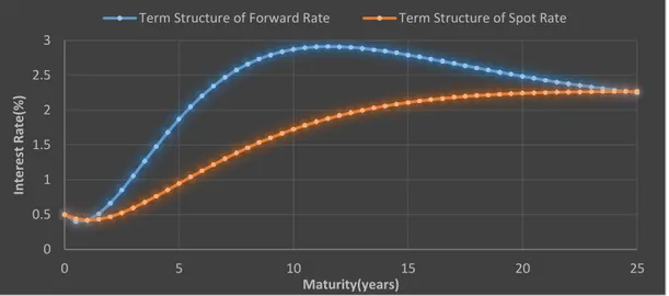
Figure 3.3: Term Structure of Forward & spot Rate by Nelson-Siegel-Svensson model, Fixed parameters are:

𝛽0= 2, 𝛽1= −1.5, 𝛽2= −9, 𝛽3= 9, 𝜏1= 3.5, 𝜏2= 5.

Figure 3.4: Components of the Nelson & Siegel Svensson forward curve

𝛽0= 1, 𝛽1= −2, 𝛽2= 4.5, 𝛽3= 9, 𝜏1= 1.5, 𝜏2= 4 Comp1=𝛽0, Comp2=𝑒𝑥𝑝 ( −𝑚 𝜏1), Comp3=( 𝑚 𝜏1) 𝑒𝑥𝑝 ( −𝑚 𝜏1), Comp4=( 𝑚 𝜏2) 𝑒𝑥𝑝 ( −𝑚 𝜏2) 0 0.5 1 1.5 2 2.5 3 0 5 10 15 20 25 In te re st R ate(% ) Maturity(years)

Term Structure of Forward Rate Term Structure of Spot Rate

0 0.2 0.4 0.6 0.8 1 1.2 0 2 4 6 8 10 M o d e l C u rv e Maturity(years)

23

3.4. Fixing the parameters of the model

Suppose we have k spot rates 𝑟𝑚𝑖for different maturities: 𝑚1, 𝑚2, … , 𝑚𝑘 and let 𝛣 = (𝛽0, 𝛽1, 𝛽2, 𝛽3, 𝜏1, 𝜏2) be the vector of parameters of Nelson-Siegel-Svensson model. Our objective is to find the optimal values of the parameters that best fit the given spot rates observed from the market by using the least square method.

𝐺 = ∑ (𝛽0+ 𝛽1( 1 − exp (−𝑚_𝜏 𝑖 1 ) 𝑚 𝜏1 ) + 𝛽2( 1 − exp (−𝑚_𝜏 𝑖 1 ) 𝑚 𝜏1 − exp (−𝑚𝑖 𝜏1 )) + 𝛽3( 1 − exp (−𝑚_𝜏 𝑖 2 ) (−𝑚_𝜏 𝑖 2 ) − exp (−𝑚𝑖 𝜏2 )) 𝑘 𝑖=1 − 𝑟(𝑚𝑖)𝑀) 2

Here 𝑟𝑀 is the observed rate from the market and 𝑟𝑁𝑆𝑆 is the estimated rate from Nelson-Siegel-Svensson model. By using the solver function in Excel and adjusting the values of vector B we obtain the minimum value for G.

By using the solver function in Excel we solve this optimization problem.

Our objective is to minimize the sum of the squared difference between estimated rates taken from Nelson-Siegel-Svensson model, and observed rates from the market.

We proceed by first setting the initial values for parameter vector 𝛣, the proper choice for initial values of vector B guarantees the convergence toward the minimum of the objective function. Our knowledge of economic interpretation of parameters of the model helps to constrain the parameters to obtain the accurate term structure.

As is mentioned in the above Section, 𝛽0 is interpreted as long-run yield level and therefore, the value of the spot

rate with longest maturity in the observed rates from market is an appropriate choice for its initial value. The contribution of the short-term component is 𝛽1, and it determines the slope of the curve. The contribution of the

middle-term component is 𝛽2 and degree of curvature is controlled by this factor.

The last expression in model [5] adds a second possible hump to the curve, and parameters 𝜏1 and 𝜏2 determine the

position of possible humps in the curve and must be positive.

After setting the initial values for the vector B, we calculate the spot rates by Nelson-Siegel-Svensson model and we find the minimum value for

𝐺 = ∑[𝑟(𝑚𝑖)𝑀− 𝑟(𝑚𝑖)𝑁𝑆𝑆]2 𝑘

24

Methodology

4.1. Curve construction of interest rate

Term structure of interest rate or yield curve plays a critical role in valuation of interest rate derivatives. It is also of a great importance to build an accurate discount curve and a smooth forward rate curve to conduct the monetary policy.

An accurate yield curve has a great influence on the performance of the traders, therefore a parsimonious model that construct the entire yield curve with high quality is of the great interest to traders and central banks.

However there is not a unique, single or standard process for constructing the yield curve from a set of observed market rates even when the curve completely reproduce the price of the given instruments. Market practice have been to use linear interpolation in trading software, which leads to a sig-saw-shaped forward curve (see Section 5.3.4), while many central banks use a Nelson-Seigel parameterization.

The challenging question is how to construct an accurate and smooth interest rate curve. The objective of this thesis is to construct the yield curve first by linear interpolation and bootstrapping and then perform the extended version of Nelson and Siegel model to observe and compare the performance ability between the models.

The yield curve is defined as the relationship between interest rates and their time to maturity. The relationship between discount factors and time to maturity is known as the discount curve. However forward rates, discount factors and yield are closely related concepts, once one is derived other ones can be determined.

One approach to construct a yield curve is to evaluate the discount factors and then extract the yield via above formulas. (In general you first calculate the zero rates and then the discount factors. The discount factors are then used as a base to construct all other rates (simple, annual compounding and with different day-count conventions)).

There is no standard model to construct a yield curve, and therefore no standard shape for the term structure of yield curve. While we directly observe some points on the curve from the market data, illiquidity of the instruments and lack of market data are challenges to form the term structure of the interest rate. To overcome these obstacles bootstrapping process and interpolation method must be applied to construct a yield curve.

25

4.2. Bootstrapping

As it mentioned in Section 2, bootstrapping is a process for extracting zero-coupon rates from a series of market prices of coupon bearing instruments such as bonds or swaps to build the yield curve. This process determines the shape of the yield curve. Banks construct different kind of curves for different kinds of trades. The rate for discounting should reflect the cost of funding for a bank. This funding is close to the interbank rate at which banks can borrow from each other.

However, the bootstrapping procedure is not the same for different instruments. But, the curves (at least when using linear interpolation) should reproduce the market prices.

In the following bootstrapping procedures for cash deposits with maturities O/N, T/N, 1week, 1month, 2 months and 3 months, forward rate agreements (FRA) and swaps with maturity from 1 year up to 30 years are described, since we are dealing with these instruments in this thesis.

Deposit rates are used for constructing the short term of the curve, FRA for short term to medium term and swap rates for constructing the longer term of the curve.

We start by calculating the discount factor and zero rate for short-term of the curve.20

𝐷𝑂/𝑁= 1 1 + 𝑟𝑂/𝑁 𝑑𝑂/𝑁 360 𝑍𝑂/𝑁= −100 ln (𝐷_𝑂/𝑁) 𝑑𝑂/𝑁 365

where 𝐷𝑂/𝑁 is the discount factor, 𝑟𝑂/𝑁 is the O/N interest rate, 𝑑𝑂/𝑁 denotes the length of the contract and 𝑍𝑂/𝑁is

the zero rate.21

We continue by calculating the discount factor and zero rate for T/N

𝐷𝑇/𝑁= 𝐷𝑂/𝑁 1 + 𝑟_𝑇/𝑁𝑃𝑎𝑟𝑑₃₆₀ 𝑇/𝑁 𝑍𝑇/𝑁 = −100 ln (𝐷𝑇/𝑁) 𝑑𝑇/𝑁 365 20

Day count convention: ACT/360

26 Discount factor and zero rate for money market instruments

𝐷𝑖 = 𝐷𝑇 𝑁 1 + 𝑟_𝑖𝑃𝑎𝑟 𝑑𝑖 360 𝑖 = {1𝑊, 1𝑀, 2𝑀, 3𝑀}. 𝑍𝑖 = −100 ln(𝐷𝑖) 𝑑𝑖 365 𝑖 = {1𝑊, 1𝑀, 2𝑀, 3𝑀}.

To calculate the discount factor and zero rate for Forward Rate Agreements we need a rate called stub rate, stub rate should have the maturity date same as the starting date of a forward rate agreement contract, and this rate can be found by linear interpolation.

𝐷_𝐹𝑅𝐴𝑖 = 𝐷𝐹𝑅𝐴 𝑖−1 1 + 𝑟_𝐹𝑅𝐴𝑖 𝑑𝐹𝑅𝐴𝑖 360 where 𝐷_𝐹𝑅𝐴0 = 𝐷𝑠𝑡𝑢𝑏, 𝑟𝐹𝑅𝐴0 = 𝑟𝑠𝑡𝑢𝑏 and 𝑍𝐹𝑅𝐴𝑖 (𝑇) = −100 𝑙𝑛(𝐷_𝐹𝑅𝐴𝑖 ) 𝑑_𝐹𝑅𝐴𝑖 365 .

Here i represents the i:th FRA contract with maturity at ti, ti < ti+1 < ti+2…

We continue with swaps to get the long-term of the yield curve. The swap par rate is given by

𝑟_𝑇𝑝𝑎𝑟=𝐷𝑇/𝑁− 𝐷𝑇 ∑𝑇𝑡=1𝑌𝑡𝐷𝑡

,

where 𝑟_𝑇𝑝𝑎𝑟 is the swap part rate with time of maturity at T, and 𝑌𝑡 is the year fraction at time t given by

𝑌𝑡 =

360(𝑦𝑡− 𝑦𝑡−1) + 30(𝑚𝑡− 𝑚𝑡−1) + (𝑑𝑡− 𝑑𝑡−1)

360 .

where 𝑦𝑡 is the year, 𝑚𝑡 is the month and 𝑑𝑡 the day for the rate.

From this we get the following formula for the discount factor

𝐷𝑇 = 𝐷𝑇/𝑁− 𝑟𝑇 𝑝𝑎𝑟_∑ 𝑌𝑡𝐷𝑡 𝑇−1 𝑡 1 + 𝑌𝑇𝑟𝑇 𝑝𝑎𝑟

27 Finally the zero rate is given by

𝑍𝑇 = −100

ln(𝐷𝑇)

𝑑𝑇

365

For the years we don’t have the swap rate we use linear interpolation to get the swap rates and from that we calculate the discount factors and zero rates.

4.3. Linear Interpolation

Let f(x) be a function, linear interpolation is an approach to approximate a value of f , defined as p(x), by using the values of two known data points, 𝑓(𝑥1) and 𝑓(𝑥2). The linear interpolation function for any 𝑥 ∈ [𝑥0, 𝑥1], is defined

as

𝑝(𝑥) = 𝑓(𝑥0) +

𝑓(𝑥1) − 𝑓(𝑥0)

(𝑥₁− 𝑥0)

(𝑥 − 𝑥0)

this equation can easily be arranged so that

𝑝(𝑥) = (𝑥 − 𝑥0) (𝑥1− 𝑥0) 𝑓(𝑥1) + (𝑥₁− 𝑥) (𝑥1− 𝑥0) 𝑓(𝑥0)

As it mentioned, illiquidity of the instruments is one of the problem in constructing the yield curve. Interpolation is one approach to complete the missing data.

Bootstrapping and interpolation method are two related procedures, interpolation complete the missing data that are proceed in bootstrapping.

Linear interpolation is popular because of its simplicity, however using the linear interpolation is a not a good approach to construct the yield curve, because of producing a zigzag shaped forward rate curve.

4.3.1. Linear interpolation on discount factor

Let 𝑡 ∈ (𝑡1, 𝑡𝑛) , so that, 𝑡 ≠ 𝑡𝑖 and 𝑡𝑖 < 𝑡 < 𝑡𝑖+1 , for 𝑖 = 1, … , 𝑛 − 1, If D(𝑡𝑖) and D(𝑡𝑖+1) are given then we can

derive D(t) by using the linear interpolation

D(t) = 𝑡 − 𝑡𝑖 𝑡𝑖+1− 𝑡𝑖 D(𝑡𝑖+1) + 𝑡𝑖+1− 𝑡 𝑡𝑖+1− 𝑡𝑖 D(𝑡𝑖)

28

4.4. Interest Rate Swap valuation (traditional approach)

Swaps are agreements between two parties to exchange a series of cash flows based on variable rates at regular intervals, these rates can be fixed or floating. The payable or receivable cash flows are commonly calculated by multiplying the reference rate or the par rate of the swap by the nominal amount, all the terms must be specified in the contract.

In the plain-vanilla swap one party agrees to pay a series of cash flows on the basis of a fixed rate while the counterpart pays the cash flows on the basis of a floating rate, commonly a LIBOR interest rate is applied on the notional amount stated in the contract. Counterparties usually don’t exchange the notional value.

Consider two bonds that one pays a fixed rate coupon and the second one pays a floating rate. The interest rate swaps can be considered as a series of zero coupon bonds, which pay a series of cash flows. To price a swap these cash flows are discounted by a zero-coupon rate corresponding to the date of the payment. The process of swaps valuation is intimately connected to discounting the future cash flows.

Define 𝑝(𝑇) as the discount factor for a cash flow at time T, and 0 = 𝑇̅̅̅, … , 𝑇0 ̅̅̅ and 0 = 𝑇𝑛 0, 𝑇1, … , 𝑇𝑚 respectively

the payment dates on the fixed and floating legs, so that 𝑇̅̅̅=𝑇𝑛 𝑚.

Let ∆𝑖= 𝑇𝑖− 𝑇𝑖−1and Δ𝑖 = 𝑇𝑖− 𝑇𝑖−1 be the length of time interval between two payment dates (day count

fraction) on the fixed and floating legs. Then 𝑝(𝑇𝑖), the discount factor is defined by

𝑝(𝑇𝑖) =

𝑝(𝑇𝑖−1)

1 + Δ𝑖𝐹𝑖

.

By solving the above equation for 𝐹𝑖, we get the forward rate for the interval [𝑇𝑖−1, 𝑇𝑖]

𝐹𝑖 =

𝑝(𝑇𝑖−1) − 𝑝(𝑇𝑖)

𝑝(𝑇𝑖)Δ𝑖

.

The cash flow (CF) for interval [𝑇𝑖−1, 𝑇𝑖] on the floating leg is determined by

CF = Δ𝑖𝐹𝑖 𝑝(𝑇𝑖) = 𝑝(𝑇𝑖−1) − 𝑝(𝑇𝑖) .

The value of the whole floating rate is then determined by

𝑉𝑓𝑙𝑡 _{= ∑{𝑝(𝑇}

𝑖−1) − 𝑝(𝑇𝑖)} 𝑚

𝑖=1

29

Consequently on the issuance date or any reset date, the value of the floating rate bond is always at par or face value.

The total value of the floating rate bond

∑𝑖=1𝑚 Δ𝑖𝐹𝑖 𝑝(𝑇𝑖) + 𝑝(𝑇𝑚) = 1 − 𝑝(𝑇𝑚) + 𝑝(𝑇𝑚) = 1 .

Values for the fixed leg

Let C be the fixed coupon rate, then the value of the fixed leg is given by:

𝑉𝑓𝑖𝑥 = ∑ 𝐶 ∆𝑖 𝑛

𝑖=1

𝑝(𝑇𝑖).

At swap’s inception there is no advantage to either party, it means that the fair value of the swap is zero and the value of the floating leg and fixed leg must be equal, that is

𝑝(𝑇̅̅̅) + ∑ 𝐶 ∆𝑛 𝑖 𝑛

𝑖=1

𝑝(𝑇𝑖) = 1 [5]

If we solve the above equation for C, we get the price of the swap, which is the interest rate that makes the floating leg have the same value as the fixed leg. This rate is the fixed payment rate of the swap.

𝐶 = 1 − 𝑝(𝑇̅̅̅)𝑛 ∑𝑛𝑖=1∆𝑖 𝑝(𝑇𝑖)

.

This rate which is known as the par rate makes the swap have the market value of zero. The same technique is used to value the swap during its life time, but over the time, forward rates change and it makes the value of the swap deviate from zero.

If we solve equation [6] for 𝑝(𝑇̅̅̅) we get the following formula which is basis for recursive bootstrapping of 𝑛

discount factor

𝑝(𝑇̅̅̅) =𝑛

1 − 𝐶 ∑𝑛−1𝑖=1 ∆𝑖𝑝(𝑇𝑖)

1 + Δ̅̅̅̅ 𝐶𝑛

.

Pricing a swap requires some key information. Tenor of the swap, day count conventions, frequency of the payments, maturity of the swap, payment dates, notional value of the swap, swap’s rate, floating rate for the current payment and whether the swap is a payer or receiver23_{, are among the required information.}

23

30

4.5. Financial crisis and its effect on pricing methodology

Sudden increase of basis spreads between similar interest rate instruments with different underlying rate tenors (swaps in particular), is among the consequences of the financial crisis or so called “credit crunch” that began in summer 2007.

Before the credit crunch in 2007, basis spreads was ignorable and therefore market segmentation was not effective, but after the financial crisis, basis spreads between similar instruments with different tenor (for example between EURIBOR and EONIA OIS swaps) significantly diverged from zero and were not negligible anymore. Therefore a new methodology and framework to price and hedge the interest rate derivatives was necessary.

Figure 4.1: Quotations for the six euro basis swap spread curves corresponding to the four Euribor swap curves 1M, 3M, 6M, and 12M. Source: Reuters, February 16, 2009

Prior to the credit crunch a single yield curve was constructed by a selection of liquid market instruments and future cash flows were generated and discounted by the same single curve, but financial crisis implied that one single curve is not sufficient for forward rates with different tenors like 1, 3, 6 and 12 months because of the large basis spread mentioned above thus a multiple “forwarding” curves is in need to account for pricing derivatives in a new framework.

31

4.5.1. Market practices for pricing interest rate derivatives in multi-curve

framework.

Denote the reset days for any swap as: T0, T1, …, TN and define Δ_𝑖 as the time interval Ti – Ti-1. (For the sake of

simplicity in calculations, assume that the payment dates for both floating side and fixed side are the same). The holder of a payer swap receives fixed payments at times T1, T2… TN, and pays at the same times floating payments.

For each period [Ti, Ti+1] the forward rate Fi+1(Ti) is set at time Ti and the cash flow for the floating side ∆i+1Fi+1(Ti)

is received at Ti+1. For the same period the cash flow for the fixed side ∆i+1 C, is paid at Ti+1 where C is the (fixed)

swap rate.

The discount factor 𝑝(𝑇𝑖), is defined by

𝑝(𝑇𝑖) =

𝑝(𝑇𝑖−1)

1 + Δ𝑖 𝐹𝑖

.

In a multi-curve framework we might generate the cash-flows with one curve (for example EURIBOR rate swap curve with 3-month tenor, as below) and discount with another (for example a EURIBOR rate swap curve with 6-month tenor, as below). Then, we have to modify the calculation as follows:

The total value of the floating side, 𝑉𝑓𝑙𝑡

𝑉𝑓𝑙𝑡 _{= ∑ Δ} 𝑖 𝐹3𝑀(𝑇𝑖−1,𝑇𝑖) 𝑝6𝑀(𝑇𝑖) 𝑁 𝑖=1 = ∑𝑝3𝑀(𝑇𝑖−1) − 𝑝3𝑀(𝑇𝑖) 𝑝3𝑀(𝑇𝑖) 𝑁 𝑖=1 𝑝6𝑀(𝑇𝑖) .

We see that we cannot simplify this as we did when using the same tenors on both curves. The total value at time t for the fixed side, using a 6-month tenor for discounting equals to:

The total value of the fixed side, 𝑉𝑓𝑖𝑥

𝑉𝑓𝑖𝑥 = ∑ Δ𝑖 𝐶 𝑝6𝑀(𝑇𝑖) 𝑁 𝑖=1 = 𝐶 ∑ Δ𝑖 𝑝6𝑀(𝑇𝑖) . 𝑁 𝑖=1

Where C is the swap rate. This is a par rate since it makes the price of the swap to be equal zero when entering the swap contract. So the total value of the payer swap (V), is given by

𝑉 = ∑𝑝3𝑀(𝑇𝑖−1) − 𝑝3𝑀(𝑇𝑖) 𝑝3𝑀(𝑇𝑖) 𝑁 𝑖=1 𝑝6𝑀(𝑇𝑖) − 𝐶 ∑ Δ𝑖 𝑝6𝑀(𝑇𝑖) 𝑁 𝑖=1 = ∑ (𝑝3𝑀(𝑇𝑖−1) − 𝑝3𝑀(𝑇𝑖) 𝑝3𝑀(𝑇𝑖) − 𝐶 Δ𝑖) 𝑁 𝑖=1 𝑝6𝑀(𝑇𝑖) .

32 With different tenors the price of the swap is given by

∑ (𝑝3𝑀(𝑇𝑖−1) − 𝑝3𝑀(𝑇𝑖) 𝑝3𝑀(𝑇𝑖) − 𝐶 Δ𝑖) 𝑝6𝑀(𝑇𝑖) = 0 𝑁 𝑖=1 𝐶 = ∑ 𝑝3𝑀(𝑇𝑖−1) − 𝑝3𝑀(𝑇𝑖) 𝑝3𝑀(𝑇𝑖) 𝑁 𝑖=1 𝑝6𝑀(𝑇𝑖) ∑𝑁𝑖=1Δ𝑖 𝑝6𝑀(𝑇𝑖) 𝐶 =1 𝑇∑ ( 𝑝3𝑀(𝑇𝑖−1) − 𝑝3𝑀(𝑇𝑖) 𝑝3𝑀(𝑇𝑖) ) 𝑁 𝑖=1 Or 𝐶 = 1 𝑇∑ ( 𝑝3𝑀(𝑇𝑖−1) 𝑝3𝑀(𝑇𝑖) − 1) 𝑁 𝑖=1 .

33

Empirical Analysis

The objective of this Chapter is to assess the adequacy and forecast performance of extended version of Nelson and Siegel model.

5.1. Data and Parameters

All data in this Section are taken from Bloomberg at 2012-11-14 and 2013-08-02. Bloomberg is used by many banks to get market data and to value complex instruments.

In order to construct the yield curves and price the swaps, I have used EONIA (Euro Overnight Index Average) rates and also EURIBOR rates with 3 months and 6 months tenors, containing O/N, T/N and cash deposits from 1 month to 3 months for short-term of the curve and Euro swap rates with maturities from 1 year to 30 years to construct the long-term of the curve, all instruments have stamp date at 2012-11-14. (Deposits, FRA and Interest Rate Swaps, are the most liquid instruments in the market, respectively with the short, middle and long term maturities)

To analyze the forecast performance of extended version of Nelson and Siegel model I have used the same instruments with stamp date at 2013-08-02.

Day count convention: ACT/360 Currency: Euro

5.2. Building the spot rate and forward rate curves

In this Section yield, forward and discount curves for selected data are built, first by using interpolation and bootstrapping methods described in details in Chapter 4 and then by Nelson-Siegel-Svensson method, the model and process of fixing the parameters are explained in details in Chapter 3.

34

5.2.1. Data

Table 5.1: EURIBOR rates at 2012-11-14, Interval: 3 Months.

Instrument

Tenor

Start date

End date

Market Rates (%)

M. Mkt.

O/N

2012-11-14

2012-11-15

0.01429

M. Mkt.

T/N

2012-11-14

2012-11-16

0.01429

M. Mkt.

1W

2012-11-14

2012-11-23

0.078

M. Mkt.

1M

2012-11-14

2012-12-17

0.108

M. Mkt.

2M

2012-11-14

2013-01-16

0.144

M. Mkt.

3M

2012-11-14

2013-02-18

0.191

FRA

3X6

2012-11-14

2013-05-16

0.16

FRA

6X9

2012-11-14

2013-08-16

0.16

FRA

9X12

2012-11-14

2013-11-18

0.18

Swap

2Y

2012-11-14

2014-11-17

0.234

Swap

3Y

2012-11-14

2015-11-16

0.346

Swap

4Y

2012-11-14

2016-11-16

0.5085

Swap

5Y

2012-11-14

2017-11-16

0.7015

Swap

6Y

2012-11-14

2018-11-16

0.9023

Swap

7Y

2012-11-14

2019-11-18

1.093

Swap

8Y

2012-11-14

2020-11-16

1.261

Swap

9Y

2012-11-14

2021-11-16

1.409

Swap

10Y

2012-11-14

2022-11-16

1.54

Swap

12Y

2012-11-14

2024-11-18

1.766

Swap

15Y

2012-11-14

2027-11-16

1.993

Swap

20Y

2012-11-14

2032-11-16

2.132

Swap

30Y

2012-11-14

2042-11-17

2.188

35

Table 5.2: EONIA rates at 2012-11-14

Instrument

Tenor

Start date

End date

Market Rates (%)

M. Mkt.

O/N

2012-11-14

2012-11-15

0.08

M. Mkt.

T/N

2012-11-14

2012-11-16

0.08

Swap

1W

2012-11-16

2012-11-23

0.082

Swap

1M

2012-11-16

2012-12-17

0.08

Swap

2M

2012-11-16

2013-01-16

0.078

Swap

3M

2012-11-16

2013-02-18

0.071

Swap

4M

2012-11-16

2013-03-18

0.065

Swap

5M

2012-11-16

2013-04-16

0.059

Swap

6M

2012-11-16

2013-05-16

0.055

Swap

7M

2012-11-16

2013-06-17

0.052

Swap

8M

2012-11-16

2013-07-16

0.05

Swap

9M

2012-11-16

2013-08-16

0.048

Swap

10M

2012-11-16

2013-09-16

0.047

Swap

11M

2012-11-16

2013-10-16

0.047

Swap

1Y

2012-11-16

2013-11-18

0.048

Swap

18M

2012-11-16

2014-05-16

0.057

Swap

2Y

2012-11-16

2014-11-17

0.085

Swap

3Y

2012-11-16

2015-11-16

0.177

Swap

4Y

2012-11-16

2016-11-16

0.333

Swap

5Y

2012-11-16

2017-11-16

0.526

Swap

6Y

2012-11-16

2018-11-16

0.715

Swap

7Y

2012-11-16

2019-11-18

0.909

Swap

8Y

2012-11-16

2020-11-16

1.076

Swap

9Y

2012-11-16

2021-11-16

1.222

Swap

10Y

2012-11-16

2022-11-16

1.351

Swap

12Y

2012-11-16

2024-11-18

1.578

Swap

15Y

2012-11-16

2027-11-16

1.809

Swap

20Y

2012-11-16

2032-11-16

1.956

Swap

25Y

2012-11-16

2037-11-16

2.00

Swap

30Y

2012-11-16

2042-11-17

2.02

36

Table 5.3: EURIBOR rates at 2012-11-14, Interval: 6 Months.

Instrument

Tenor

Start date

End date

Market Rates (%)

M. Mkt.

O/N

2012-11-14

2012-11-15

0.01429

M. Mkt.

T/N

2012-11-15

2012-11-16

0.01429

M. Mkt.

3 M

2012-11-16

2013-02-18

0.191

M. Mkt.

6 M

2012-11-16

2013-05-16

0.358

Swap

1 Y

2012-11-16

2013-11-18

0.34

Swap

2 Y

2012-11-16

2014-11-17

0.389

Swap

3 Y

2012-11-16

2015-11-16

0.495

Swap

4 Y

2012-11-16

2016-11-16

0.655

Swap

5 Y

2012-11-16

2017-11-16

0.847

Swap

6 Y

2012-11-16

2018-11-16

1.043

Swap

7 Y

2012-11-16

2019-11-18

1.226

Swap

8 Y

2012-11-16

2020-11-16

1.39

Swap

9 Y

2012-11-16

2021-11-16

1.533

Swap

10 Y

2012-11-16

2022-11-16

1.66

Swap

12 Y

2012-11-16

2024-11-18

1.877

Swap

15 Y

2012-11-16

2027-11-16

2.093

Swap

20 Y

2012-11-16

2032-11-16

2.218

Swap

25 Y

2012-11-16

2037-11-16

2.246

Swap

30 Y

2012-11-16

2042-11-17

2.255

Source: Bloomberg,

37

5.3. Fitted Curves

Based on the Euribor rates with various tenors O/N, to 30 years from 2012-11-14 to 2042-22-17 (see Table 5.1, 5.2 and Table 5.3), the yield, forward and discount curves are shown in the following Figures.

5.3.1. Yield Curves

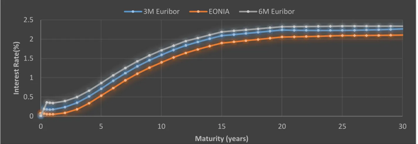
Figure 5.1: Plot of fitted yield curves for 3M Euribor rates, together with actual market rates, (Table 5.1)

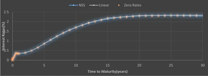
Figure 5.2: plot of fitted yield curves for EONIA rates together with actual market rates, (Table 5.2)

0 0.5 1 1.5 2 2.5 0 5 10 15 20 25 30 In te re sr r ate (% ) Maturity (years)

Linear Interpolation NSS Method Zero Rates

0 0.5 1 1.5 2 2.5 0 5 10 15 20 25 30 In ter est rat e( %) Time to Maturity(years)

38

Figure 5.3: plot of fitted yield curves for 6M Euribor rates together with actual market rates, (Table 5.3)

As we see in above Figures time to maturity for all curves span to 30 years, from 2012 to 2042, both NSS and interpolation method generate smooth yield curves, both curves generated by interpolation method and NSS model almost completely overlap.

5.3.2. Forward Curves

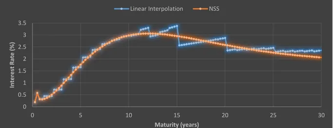
Figure 5.4: 3M Forward Curves for 3M Euribor rates built by linear interpolation and NSS model (Table 5.1)

0 0.5 1 1.5 2 2.5 0 5 10 15 20 25 30 In ter est R at es( %) Time to Maturity(years)

NSS Linear Zero Rates

0 0.5 1 1.5 2 2.5 3 3.5 0 5 10 15 20 25 30 In ter est R at e( % ) Maturity (years) Interpolation NSS