Welfare effects of Stockholm congestion charges
using dynamic network assignment
Maria Börjessona and Ida Kristofferssonb
Abstract
According to the standard textbook analysis, drivers as a group will be worse off with congestion charging if not compensated by revenues. This result is confirmed by an analysis of the Stockholm congestion charging scheme using a static model with homogenous users. However, both this static model and the standard textbook analysis omit three important factors: taste heterogeneity, effects of charges on the larger network arising from less blocking back of upstream links and behavioural adjustments in the temporal dimensions. Taking account of these factors, using a dynamic model with heterogeneous users in a large-scale network, we find that drivers as a group benefit directly from the charging scheme in Stockholm. This paper investigates the importance of the three factors omitted in the standard textbook and the static model analysis in the Stockholm case, finding that all three add significantly to the benefit of the charges.
Keywords: Congestion charges, Congestion pricing, Road pricing, Acceptability, Evaluation, Urban transport policy, Mobility management, Transport externalities, Policy implementation
amaria.borjesson@abe.kth.se, Centre for Transport Studies, KTH. b
ida.kristoffersson@abe.kth.se (corresponding author), Dept. of Transport Sciences, KTH, Teknikringen 72, SE-10044 Stockholm, Sweden. Phone: +46 8 790 84 25, Fax: +46 8 21 28 99.
2
1.
Introduction
It is generally known that congestion charging can be an effective measure to solve environmental and congestion problems in urban areas, but there is still low political and public acceptability in many urban area. One possible reason for low acceptability is the notion that drivers are worse off if not compensated by the revenues. In fact, the standard textbook analysis of congestion charging (Walters, 1961), using a static model of one origin and one destination connected by one link and homogenous users, shows that drivers are worse off with congestion charges if not compensated by return of revenues. This result is confirmed by an analysis of the Stockholm congestion charging scheme using the national traffic model “Sampers”, homogenous1 users and static network assignment (Engelson and van Amelsfort, 2011).
Both the Sampers and the standard textbook analysis disregard three important factors increasing the benefits of congestion charges: network effects, preference heterogeneity and dynamics in the temporal dimension. First, network effects imply that travellers who do not pay charges may benefit from them. Network effects are disregarded in the standard textbook analysis and greatly underestimated in static network assignment models that fail to model blocking back of upstream links as queues builds up. Second, ignoring heterogeneity in value of travel time savings (VTTS) in a system with a free parallel road leads to great underestimation of benefits because efficiency gains due to separation of traffic are ignored (Verhoef and Small, 2004). Third, in a one-link dynamic bottleneck setting with homogenous users Arnott et al. (1994) show that an optimal time varying congestion charge is welfare neutral for drivers if not compensated by return of revenues, since the reduction in queuing costs exactly compensates the charge.
The purpose of this paper is to estimate to what extent the three factors discussed above add to the social benefit of the Stockholm congestion charging scheme, and a slightly modified scheme, using the model “Silvester”, which links a dynamic network assignment model with a mode and departure time choice model assuming heterogeneous users (Börjesson, 2008; Kristoffersson and Engelson, 2009). We find that each factor add significantly to the benefit of the charging scheme. In fact, the Silvester analysis indicates that drivers benefit directly from the congestion charging scheme, without compensation. Direct benefits for many drivers could be one factor explaining the high public support for the congestion charges in Stockholm, which has even increased since the congestion charging scheme was introduced in 2006 (Börjesson et al., 2010).
There is a large literature studying welfare effects of congestion charges. Most of the literature is theoretical (Verhoef and Small, 2004; Arnott et al., 1994; Glazer and Niskanen, 2000; Evans, 1992). There are also a few studies on real-world congestion charging schemes, most of them based either on observed travel times or on travel times from static assignment models. Eliasson (2009) provides an a posteriori cost-benefit analysis of the Stockholm congestion charges, based on observed travel times. Eliasson’s study results in a net benefit of about 80 M€/year and as much as 40% of the time gains arise outside the cordon. Santos and Shaffer (2004) present and discuss a cost benefit analysis of the London congestion charging scheme undertaken by Transport for London (TfL), which is also based on observed travel data. Prud’homme and Bocarejo (2005) have undertaken another cost-benefit analysis of the London congestion charging scheme based on observed data. The results of the two analyses for London are very different: TfL finds a net benefit of the charging system of about 70 M€/year (similar to the result for Stockholm given above), whereas Prud’homme and Bocarejo find a net loss of about the same size. The main difference in the two studies lies, according to Mackie (2005) and Raux (2005), in
1
On the demand side Sampers is segmented into six trip purposes within which users are homogeneous. On the supply side five VTTS classes are used in assignment.
3
calculation of travel time savings and the VTTS. Prud’homme and Bocarejo (2005) do not consider travel time savings outside of the charging zone and apply a lower VTTS.
Two independent cost benefit analyses have been made of a proposed marginal social cost pricing scheme in the Oslo-Akershus metropolitan region, which has a population of about one million. Grue et al. (1997) find a social benefit of 49 €/capita/year2 for the Oslo-Akershus area. The benefit is somewhat higher, 75 €/capita/year, in Fridström et al. (2000). The higher benefit in Fridström et al. (2000) is according to Vold et. al (2001) due to the fact that the transport models differ and because the cost-benefit analysis is somewhat simpler in Grue et al. (1997). The difference in the transport models is not in assignment; both use the static Emme/2 model. Rather, the two models differ on the demand side, where the model used in Fridström et al. (2000) includes trip frequency, destination and mode choice, whereas the model used in Grue et al. (1997) includes on the demand side route and departure time choice.
Rich and Nielsen (2007) provide social benefit calculations of four proposed charging schemes in Copenhagen using advanced route choice models but not dynamic assignment. Maruyama and Sumalee (2007) compare social benefit of different charging schemes in Utsunomia in Japan using volume-delay functions to calculate link travel times, i.e. static assignment. The conclusion in Maruyama and Sumalee (2007) is that area-based schemes are in general socially more beneficial, but also more inequitable than cordon-based schemes. Kickhöfer et al. (2010) provide social benefit calculations of several proposed distance-based charging schemes in Zürich using the activity-based model Matsim.
It is well known that congestion pricing normally will generate a net welfare surplus, but different researches have come to different conclusions as to whether congestion charges will be progressive or regressive. The conclusion is largely dependent on what assumptions are made about the distributions of VTTS, scheduling preferences and flexibility (Verhoef and Small, 2004; Arnott et al., 1994). It is also dependent on whether citizens have access to and actually patronize public transport and "slow modes" and how the revenues are used (Verhoef and Small, 2004; Glazer and Niskanen, 2000; Armelius and Hultkrantz, 2006). The distributional effects are not the main focus of this paper. However, in the study of welfare effects we are touching upon distributional effects when analysing gains and losses of different groups of travellers. The distributional effects are important, since it is critical to design congestion charges such that a large proportion of the population perceives themselves as winners in order to gain acceptability from the public, as noted by several authors (Arnott et al., 1994; Eliasson, 2008).
The Stockholm congestion charging scheme consists of a cordon around the inner city, reducing traffic through the bottlenecks located at the arterials leading into the inner city. In this paper we also analyse a slightly modified version of the scheme that will be introduced at a later stage, which generates substantial higher benefits than the present system. The charging trial has been described in detail elsewhere (Börjesson et al., 2010; Eliasson, 2008; Eliasson et al., 2009). Since it is usually assumed that drivers are not fully compensated by shorter travel times, the recommendation in the acceptance literature is that congestion charges must be part of a ‘‘package’’ and that the acceptance will be strongly dependent on how the revenues are used (Eliasson, 2008). The present study suggests that this may not always be the case, since many drivers may benefit even if not compensated by the revenues. One of the most interesting and encouraging results of the Stockholm congestion charges in Stockholm has been the positive trend in public and political support of the charges to the extent that acceptability is no longer an issue. In Stockholm municipality the public support has gradually risen from less than 30 % in favour of the charges to slightly more than 50 % at the end of the trial, and to almost 70 % at the end of 2007.
2
4
The outline of this paper is as follows. A theoretical background is given in the next section, followed by a description of the dynamic modelling system Silvester in section 3. Section 4 describes the congestion charging scheme in place in Stockholm today and the modified version that is analysed in this paper. Section 5 describes the methods and results are given in Section 6. Section 7 concludes.
2.
Theory
In the standard textbook analysis (Walters, 1961), it can easily be shown that all drivers paying a congestion charge are not fully compensated by shorter travel times. Let the total generalized cost of travelling on the link be given by Equation (1):
(1)
In Equation (1), flow is and is average generalized cost. The marginal generalized cost of additional traffic on the link is then given by Equation (2):
(2)
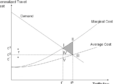
The traffic flows will, in the case without the congestion charge, increase up to the point of intersection between the average generalized cost curve and the demand curve (point in Figure 1). This is not an efficient allocation of recourses. To reach efficiency, traffic flow must decrease to the point , which is the flow corresponding to the point of intersection between the marginal generalized cost curve and the demand curve (point in Figure 1).
Figure 1:Optimal congestion charge in the static analysis of one origin and one destination connected by one link and homogeneous users.
5
To lower the flow to , the average generalized cost, , can be increased to equal the marginal generalized cost at flow by adding an optimal charge . At flow the marginal generalized cost is = and the average generalized cost is . The optimal charge is thus * = . Drivers staying on the road will pay *, but their generalized travel cost (except the congestion charge) decreases by only . Since the drivers remaining on the road will be worse off than without charges. The remaining group of drivers will lose the area [ -IV-I- ]. Drivers priced off the road lose the area under the demand curve [IV-I-III]. The net benefit of the congestion charges is the area [ -V-I- ] (revenues) minus the area [ -IV-I- ] (loss for the remaining drivers) and minus the area [IV-I-III] (loss for drivers priced off the road), which equals the area [I-II-III] (see for instance Johansson and Mattsson (1995)). The standard textbook analysis described above disregards several important factors, opening for the possibility that some drivers become better off in a situation with congestion charges.
First, the standard analysis assumes that there is one single origin-destination pair connected by one link. In a network setting the benefit could increase due to route choice effects (still assuming one origin-destination pair) or due to the fact that there are many origin-destination pairs. If route choice in user optimum is different from that of the system optimum, first-best pricing may add to the welfare of the drivers (assuming no compensation by revenues). Braess' paradox (Braess, 1968) constitutes a good example, stating that an additional link in a network in some cases increases the total travel time in the network due to inefficient route choice at user optimum. Total travel time increases because traffic using the additional link produces additional external costs in the network. If a congestion charge on the additional link internalizes the external cost in the network, the traffic flow at the additional link will become zero and the total travel time would return to the situation without the additional link, so that the drivers as a group could benefit (without paying any charge). Another situation arises if travellers have different origin-destination pairs. Verhoef and Small (2004) note that the benefit of first-best pricing on one link in a network is usually underestimated if the traffic on this link gives rise to external costs for traffic having other origin-destination pairs. The simple network of Figure 2 demonstrates the insight.
Figure 2: A simple network for illustration of network effects.
Some drivers travel (A,B) and other drivers travel (A,C). An optimal congestion charge on the link (B,C) could benefit drivers travelling from A to B. If there is blocking back of upstream links and signal plans at intersections in (A,B), which builds up from bottlenecks in (B,C), the benefit for drivers travelling from A to B may be large even if there is no capacity constraint on the link (A,B).
Second, ignoring heterogeneity in VTTS in a system with a free parallel road (or an efficient public transport system) leads to great underestimation of social benefits, by disregarding the efficiency gains due to separation of traffic (Verhoef and Small, 2004). Specially, congestion charging tends to sort trips between routes and modes with respect to VTTS. Using numerical simulations and a simple network, Verhoef and Small (2004) analyse the benefit of the second-best charging scheme with one of two parallel links charged. They find that travellers with the highest VTTS benefit from congestion charging without compensation by return of revenues. Travellers with the trade-off VTTS incur the greatest losses.
Third, in a dynamic setting the congestion charge may be time varying and the drivers’ possibility to adjust their departure time is taken into account. Arnott et al. (1994) show, assuming a one-link bottleneck model and homogenous users, that with an optimal time varying charge users adjust their departure time such that queuing is completely avoided. Moreover, they show that the optimal time varying congestion charge is welfare neutral for the drivers if they are not compensated by return of
6
revenues; the reduction in queuing cost exactly compensates the charge. If drivers have heterogeneous scheduling preferences, still assuming constant VTTS, benefits from the charges would increase even more, due to sorting of travellers with high and low scheduling costs. Hence, drivers as a group could even benefit without return of revenues. Applying a one-link bottleneck model, De Palma and Lindsey (2002) show that if the value of schedule delay (VSD) is homogenous and only the VTTS heterogeneous, all drivers lose from first best pricing, except those with the highest VTTS. Still, there is an efficiency gain due to the sorting of trips with respect to VTTS between departure times, compared to the situation when the VTTS is homogenous. Lindsey (2004), analyse the case when both VTTS and VSD vary between discrete groups. Van den Berg and Verhoef (2011) extend the work by Lindsey (2004) and consider a situation with continuously distributed VTTS and VSD. They find that travellers with an intermediate VSD and the lowest VTTS for this VDS suffer the greatest loss, both in the first-best pricing case and the second-best case with a free parallel road. In the second-best case, also those with low VSD may substantially benefit from the second-best scheme, attracted to the earliest and latest departure times on the tolled road.
Fourth, the textbook analysis neglects the benefit of improved travel time reliability due to congestion charging. In the analysis of travel time reliability, there are two principally distinct approaches: the “scheduling approach”, where the traveller’s departure and arrival time preferences are made explicit in the model; and the “reduced-form approach”, where some statistical measure of the variability in travel times is introduced directly in a reduced-form indirect utility function. Fosgerau and Karlström (2010) derive a reduced-form approach from an underlying scheduling model, assuming that travel times follow a known random distribution and that travellers choose their departure time optimally given this distribution. Different underlying scheduling models imply different statistical measures of reliability. Assuming the classical scheduling model originating from Vickery (1969) and Small (1982), Fosgerau and Karlström (2010) show that at the optimal departure time, the disutility of travel time unreliability is proportional to the standard deviation of travel time distribution3. Hence, in a static model, travel time reliability may be introduced in the indirect utility function as a standard deviation (or some other statistical measure depending on the underlying scheduling model) under the assumption that the travellers depart at optimal departure time4. Introducing travel time reliability as a reduced form measure can, however, not change the basic feature of the textbook example that drivers as a group become worse off with congestion charges assuming compensation by the revenues. The effect is only that the generalized cost functions become steeper in Figure 1. In a dynamic model, the reduced form is not applicable and the scheduling approach is difficult to handle in a large-scale modelling system. Many travel times must be simulated, and then departure time will adjust depending on the distribution of the travel times. It is not clear whether convergence can be reached5. Hence, in the analysis of this paper we leave the effect of travel time reliability.
Fifth, benefits from improved urban environment may arise also from the congestion charges (Eliasson, 2008). This benefit is difficult to value and we do not analyse this benefit further.
3
Given that scheduling preferences and standardized travel time distribution remains constant.
4
Given a relationship between travel time delay and the appropriate measure of reliability. 5
There are scheduling models, for instance, the one suggested by Tseng and Verhoef (2008), where the optimal departure time does not depend on the standard deviation of the travel time distribution, and only on the mean travel time.
7
3.
The model
In this section we describe the Silvester model, which will be used for analysis in this paper. The Silvester model avoids the drawbacks listed in the previous section since it includes dynamic assignment, heterogeneity in preferences within each trip purpose and possibility to change departure time. Silvester consists of two main parts which are linked in an iterative procedure. The mesoscopic dynamic assignment model Contram calculates route choice and resulting travel time and monetary cost for trips in each origin-destination pair, given the demand for car trips departing in each fifteen minute interval. A mixed logit model for departure time and mode (car or public transport) then takes the travel times and costs from the assignment model and generates the demand for car trips departing in each fifteen minute interval. The generated demand is then fed back into the assignment model.
3.1 Departure time and mode switch model
The demand model in Silvester has been estimated on stated and revealed preferences of car users in Stockholm before the introduction of charges (Börjesson, 2008). It is a mixed logit model which builds on the scheduling models of Small (1982) and Vickrey (1969), assuming that drivers trade-off travel costs (travel time, distance-based cost, charge etc.) against scheduling delay costs.
There are three trip purposes in Silvester, with one demand model for each trip purpose: 1) commuting trips with fixed working hours and school trips (short: fixed), 2) business trips (business) and 3) commuting trips with flexible working hours and other trips (flexible), where “other trips” includes e.g. shopping and leisure trips. Equation (3) shows the utility functions, which are similar for the three trip purposes, except that for business trips the public transport alternative ( ) is not available.
(3)
In Equation (3), is the utility function for public transport mode ( ) and trip purpose , is the utility function for car mode ( ) trip purpose and departure time interval . Index denotes departure times before 6.30 am, denotes departure times in the twelve quarters from 6.30 to 9.30 am respectively and departure times after 9:30 am. and are schedule
deviation early and late respectively for departure time . Since time is divided into 15 minute time intervals, and are multiples of 15 minutes. is monetary cost which includes both the congestion charge and a distance-based cost, is travel time, is standard deviation of travel time, is a Gumbel distributed error term, is an alternative specific constant for public transport and is the
share of car users who also possess a public transport monthly card (in the estimation was a dummy variable equal to if the driver had a public transport monthly card and otherwise). is the preferred departure time interval.
The demand model does not attempt to be a complete mode choice model, since it has been estimated based on data from car users only. Rather it is a mode switch model, which forecasts the share of car users switching to public transport due to changes in the network, such as introduction of congestion charges. However, as it is a logit model, it will always predict at least a small share of users choosing each alternative. Therefore, some users choose the public transport alternative already in the
8
situation without congestion charges. This share is however small in the Stockholm application and amounts to only 1.6 per cent of all users.
Parameters labelled are heterogeneous in the population following a Johnson’s SB distribution bounded on , whereas parameters labelled are assumed to be constant in the population. Heterogeneous parameters are simulated using 50 random draws from Johnson’s SB distribution. The original demand models included a normally distributed error term for the alternative specific constant
which had a large spread. Using 50 draws, the effect of this parameter depended too much on the
specific draws made. The public transport error term was therefore removed and the alternative specific constant adjusted accordingly.
Table 1: Parameter values in the departure time and mode choice models for the three trip purposes
Parameters Flexible Fixed Business
β1 (Schedule delay early, mean) -0.46 -0.35 -0.25
β2 (Schedule delay late, mean) -0.52 -0.56 -0.35
β3 (Cost, mean) -0.30 -0.26 -0.12
b1 (Travel time) -0.23 -0.08 -0.19
b2 (Travel time uncertainty) -0.09 -0.09 -0.13
b3 (PT travel time) -0.19 -0.24 - b4 (PT season ticket) 18.33 16.74 - Cp (PT constant) -3.00 3.00 - Mean VTTS in €/h 10.5 [1.6, 82.5] 8.3 [0.6, 77.2] 36 [1.6, 100] Overall mean VTTS 12.4 Percent of users 60 30 10
Parameter values for the different trip purposes are reported in Table 1. For random parameters the reported value corresponds to the mean of the draws used in simulation. The Johnson’s SB distribution is censored in order to be able to calculate a robust welfare measure based on VTTS (which is the time parameter divided by the random cost parameter). The censoring is made at VTTS equal to 100 €/h, which corresponds to a cost parameter value of for flexible trips, for fixed trips and for business trips. The simulated parameter values that are smaller than the threshold are set to the threshold. The mixed logit choice probabilities are simulated by calculating the logit formula for each draw and averaging the result (Train, 2003).
3.2 Assignment
Contram takes as input a time-sliced origin-destination matrix (OD-matrix) and a network specification, assigns vehicles to the network in the form of packages and calculates the shortest path for each package by assigning them one by one to the network (Taylor, 2003). Iteration of assignment is needed since the shortest path and corresponding travel time of a package may be affected by subsequent packages travelling between other origin-destination pairs. The iteration process can be compared to a day-by-day learning of network conditions. The naïve user chooses the shortest route under free-flow conditions, which creates sever congestion on some routes. New routes are then chosen on the second day (second iteration), given the experienced travel times from day one. After a number of days the user equilibrium is reached. Contram uses deterministic assignment such that results are always the same given the same input and scenario settings.
A description of the implementation of the Silvester demand model and the procedure of connecting the demand model to Contram is found in Kristoffersson and Engelson (2009). Silvester has been calibrated to the situation before charges were introduced in Stockholm, using a method of reverse
9
engineering, where demand in each preferred departure time interval is adjusted such that Silvester produces correct traffic flows in the no toll situation (Kristoffersson and Engelson, 2008). After validation (Kristoffersson, 2011) some additional calibration was made to reduce departure time choice effects.
4.
The congestion charging schemes
The Stockholm congestion charges were first introduced as a trial 3 January – 31 July 2006, followed by a referendum in the City of Stockholm6. The referendum was pushed through by parties against congestion charges but in the end a majority voted for keeping the charges. The new Liberal-Conservative government reintroduced the charges in August 2007. However, the revenues from the permanent system were earmarked to a partially government-funded transport investment package including both road and public transport investments.
The congestion charging scheme consists of a cordon around the inner city of Stockholm with time-differentiated charges. The congestion charge is a tax levied on certain vehicles for passages in and out of Stockholm’s inner city weekdays 6.30 am to 6.30 pm. During the trial, the traffic flows across the cordon were reduced by on average 22 percent during charged hours. The charge varies between €1 and €2 depending the time of day, with a maximum daily charge per vehicle of €6. The charge does not apply overnight, at weekends and on public holidays or during the month of July.
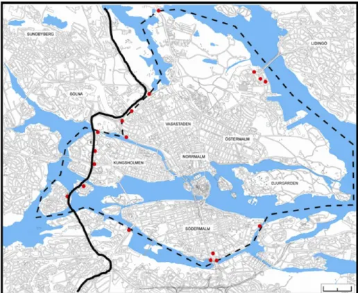
Figure 3: The cordon around the inner city of Stockholm (dashed line), the bypass E4/E20 (solid line) and the location of the charging points (red dots). Source: Eliasson et al (2009).
The area inside the cordon is around 30km2. The location of the cordon is depicted in Figure 3. The dashed line is the charging cordon, the dots are charging points and the solid line is the non-charged
6
10
bypass E4/E20 west of the inner city. There is no congestion charge for journeys to and from the island of Lidingö (see figure 3) which pass in and out of the charging zone within 30 minutes. Bypass E4/E20 is heavily congested but is not charged at present for political reasons. There is, however, political consensus for charges on the Bypass E4/E20 in 2020, when a new bypass further west is built. In this paper, we analyse primarily the modified scheme with charging levied also on the bypass E4/E20, because the welfare effect of this modified scheme is considerably higher and because this system will be introduced at a later stage. Throughout this paper, we refer to the original scheme as the “current scheme” and to the original scheme plus a charge levied on the bypass E4/E20 as the “modified scheme”. There are moderate route choice effects of the schemes, in particular in the modified scheme. In the current scheme, the main route choice effect is that drivers travelling between Northern and Southern Stockholm may choose to travel through the city centre or to divert to the bypass E4/E20 to avoid paying the charge. This effect is small in the current scheme and even smaller in the modified scheme, since a congestion charge is then also levied on the bypass E4/E20.
The revenues from charges in 2008 amounted to approximately 85 M€ in 2008. The operating cost of the current cordon scheme is approximately 25 M€ per year.
5.
Method of analysis
The Stockholm congestion charging scheme, and the modified scheme described in Section 4, have previously been analysed with the static forecast model Sampers (Engelson and van Amelsfort, 2011), which have several common features with the standard textbook analysis: network effects from congestion charges are small because the blocking back of upstream links are not modelled, within trip purposes users are assumed to have homogenous preferences and the temporal dimension is left out. The implications from the standard textbook analysis, that drivers are considerably worse off with congestion charges (before return of revenues), are also confirmed in the Sampers analysis. For these reasons, the Sampers analysis can be interpreted as an application of the standard textbook analysis of the Stockholm congestion charging schemes.
The analysis in Silvester extends the standard textbook and the Sampers analysis by including network effects, preference heterogeneity and the temporal dimension. The aim of the following analysis is to assess to what extent these effects adds to the benefit of the modified scheme in Stockholm. This is accomplished by first calculating the consumer surplus (CS) of the scheme with the standard Silvester model. We then investigate how CS changes when the three effects extending the textbook analysis are taken out from the Silvester model successively in different steps. These steps are described in sub-section 5.2-5.4. When the three effects are taken out of Silvester, the model resembles the forecast model Sampers and the standard textbook analysis. We therefore also compare CS predicted by Silvester and by Sampers. We focus on the modified scheme in this analysis.
5.1 CS calculation
First, we compute the consumer surplus of the current and modified congestion charging schemes. The CS is defined as the difference between the logsums computed with and without the scheme. The logsum is given by Equation (4):
(4)
11
and are the representative utility functions for a traveller departing at with trip
purpose , OD-pair ω, preferred departure time interval and set of preferences , defined in Equation (3). For each and , travellers are divided into 50 groups with different sets of preferences for , and . The 50 sets of preferences are constructed by combining (for each trip purpose ) 50 random draws from each of the random preferences , and . The draws are the same each time the model is applied.
When referring to CS in the rest of the paper it is assumed that no revenues are recycled.
5.2 Network effects
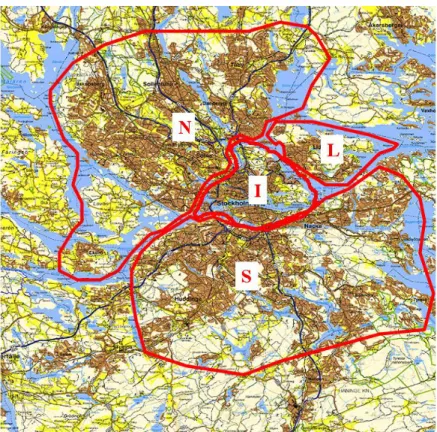
Next, we assess the benefits from network effects, arising due to the fact that travellers have different origins and destinations, by exploring to what extent the benefits accrue to drivers in trip relations where charges do not apply. To define uncharged trip relations, all trips are categorized with respect to the origin and destination zones depicted in Figure 4: Inner city (I), North zone (N), South zone (S) and Lidingö Island (L). This makes four times four origin/destination relation categories, of which eight are uncharged.
Figure 4: Stockholm divided into inner city (I), northern suburbs (N), southern suburbs (S) and Lidingö (L). The trips to and from the city centre are charged (I-N; I-S; I-L; N-I; S-I; L-I). Trips from the North zone to the South zone are charged once or twice depending on the route choice in the modified scheme (N-S; S-N). Remember that drivers travelling between the North zone and the South zone can choose the route through the city centre and pay the charge twice or the route via bypass E4/E20 and pay once. Trips to/from Lidingö from/to North zone or South zone are uncharged (N-L; S-L; L-N; L-S), as well as trips within zones (I-I; N-N; S-S; L-L).
Since the effect of route choice is limited in the modified scheme, the route choice effects would not be the main reason for the large benefits of congestion charging scheme and this is not analysed further.
12
5.3 Heterogeneous VTTS
Next, we explore to what extent the assumption about heterogeneity in VTTS adds to the benefit of the congestion charging scheme due to sorting of trips over modes and departure times with respect to VTTS. This is explored by comparing the CS computed by Equation (4) with the CS computed under the assumption that the VTTS is constant across trips. We carry out the latter computation by constraining the cost parameters ( ) to be constant over all trips with the same purpose ( ). The cost parameters for different trip purposes are chosen such that the VTTS is equal across purposes (the travel time parameter varies across trip purposes). The cost parameters are also chosen such that the model predicts the same share of traffic across the cordon diverting to public transport as in the charged situation in the standard Silvester model. The result is a VTTS of 4.8 €/h7. We may think of this VTTS as that which would have been estimated based on traffic levels before and after the introduction of congestion charges. The logsum, with and without charges, is computed as described by Equation (5), in which the cost parameter no longer depends on . Scheduling parameters are still heterogeneous (dependent on ) and therefore the logsum is still averaged over .
(5)
Efficiency gains arising from heterogeneity in VTTS will apply primarily to traffic paying the congestion charges. Sorting of trips with respect to VTTS will not occur for uncharged trip relations, since these do not face the trade-off between money and time when making the choice of mode and departure time. For this reason, the benefits arising from heterogeneous VTTS are assessed only for the charged trip relations (I-N; I-S; I-L; N-I; S-I; L-I; N-S; S-N).
5.4 Scheduling benefits
As mentioned, part of the efficiency gains due heterogeneity in VTTS is the sorting of trips in the temporal dimension since the charging system is time varying. In the next step we investigate to what extent the benefits in the dynamic model arise because travellers may reschedule. We concentrate on the benefits over and above the rescheduling benefits arising due heterogeneous VTTS captured in the analysis described in the previous section. For this reason the VTTS is held constant when further investigate the scheduling benefits.
We compute the CS under the assumptions that drivers cannot change departure time, only mode and route, when the scheme is introduced. For each group of travellers with identical preferences ( ), origin-destination pair ( ), trip purpose ( ) and preferred departure time ( ), the share of drivers ( ) departing in interval in the uncharged situation ( ), are in the charged situation constrained to go by car in the same departure time interval or to switch to public transport. Hence, the possibility to change departure time and still drive when the charges are introduced is no longer available in the model. Drivers are thus constrained to the binary choice of driving (in departure time interval ) or divert to public transport. The share of drivers travelling with public transport in the situation without charges ( is assumed to remain on public transport (this share is small in the present population, as discussed in Section 3.1). Equation (6) shows the logsum computed in the
7
13
scenario with charges. Note that the cost parameter ( ) does not depend on , since what we evaluate here is the benefit of scheduling assuming constant VTTS.
(6)
For the situation without congestion charging the logsum is computed by Equation (5). The CS of the scheme (assuming homogeneous VTTS and no scheduling benefits) is computed as the difference between these two. We do not re-run the assignment model in this analysis, and make thus the assumption that the traffic flows in each time period remain the same when departure time choice is held constant. As will be shown, this assumption seems to hold at a sufficient level.
6.
Results
6.1 CS of the schemes
We find that the total CS for all trips calculated from Equation (4) is positive, both for the current scheme and the modified scheme (current scheme plus a charge on the Bypass E4/E20). Table 2 shows the total CS of the two schemes and the total CS for each trip purpose. Table 3 shows CS per trip for all trips and for each trip purpose.
Table 2: Resulting CS forecasted by Silvester
CS, all trips (M€/year) Total Flexible Fixed Business
Current scheme 13 -2 -5 20
Modified scheme 32 4 -5 33
Business travellers gain most from the charging scheme, fixed schedule travellers least and flexible schedule travellers are in between. This is consistent with the finding of van den Berg and Verhoef (2011), who show that it is the drivers with intermediate VSD and low VTTS for this VSD that incur the greatest losses. Drivers with fixed working schedule have a VSD that is on average higher than travellers with flexible schedule and lower than business travellers. Also, they have the lowest VTTS. Furthermore, Table 3 shows that the benefit is considerably larger for the modified scheme. In this scheme, only fixed trips become worse off as a group due to the charges.
Table 3: CS per trip
CS, all trips (€) Average Flexible Fixed Business
Current scheme 0,04 -0,01 -0,06 0,67
Modified scheme 0,11 0,03 -0,06 1,11
For comparison, CS of the two schemes computed with the rule of a half and based on Sampers forecasts can be found in
Table 4. The Sampers forecast gives, as mentioned before, a large negative CS. The implications from the standard textbook analysis that drivers are worse off without return of revenues are thus confirmed. In fact, the revenues in the Sampers forecast barely balance the large negative consumer surplus.
14
Table 4: Resulting CS based on Silvester and Sampers forecasts. Source: Engelson and van Amelsfort (2011)
CS, all trips (M€/year) Silvester Sampers
Current scheme 13 -76
Modified scheme 32 -97
In the following we concentrate on the modified scheme. We refer to the CS of this modified scheme computed with the standard Silvester model as the base case CS.
6.2 Network effects
Table 5 shows the resulting CS arising for the 16 different trip relations. The larges benefits arise in uncharged trip relations: inside the cordon (I-I), within the North zone (N-N) and within the South zone (S-S), with benefits of 9.0, 14.0 and 5.2 M€/year respectively. The charges also do not apply to trips in the relations to/from North and South from/to Lidingö (N-L, L-N, S-L, L-S), and these travellers also benefit a total of 3.9 M€/year.
Table 5: CS divided on charged and uncharged trip relations
Ori
gi
n
Destination Consumer surplus all trips =
31.8 M€/year
Inner city (I) North (N) South (S) Lidingö (L)
Inner city (I) 9.0 -4.0 -8.5 -0.4
North (N) -0.5 14.0 -3.3 1.8
South (S) 7.7 11.1 5.2 1.2
Lidingö (L) -2.2 0.6 0.3 -
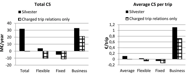
Figure 5 compares the base case total and average CS with the CS of the charged relations. The left chart shows total CS and the right shows average CS. In the charged relations, CS is negative with a total of 0.3 M€/year.
Figure 5: CS in the standard Silvester model for all trips (black) and in charged trip relations (chequered). -20 -10 0 10 20 30 40
Total Flexible Fixed Business
M € /y e ar Total CS Silvester
Charged trip relations only
-0,2 0 0,2 0,4 0,6 0,8 1 1,2
Average Flexible Fixed Business
€
/tr
ip
Average CS per trip
Silvester
15
Only business trips still have a positive CS when looking solely at charged relations. Trips with fixed schedule still incur the greatest loss both in total and per trip. The difference in CS between business trips compared to trips with fixed schedule decreases from 1.17 to 0.85 €/trip, but the difference is still substantial. The reason for the larger difference when uncharged relations are included is that business trips have a higher average VTTS, which leads to a higher valuation of the travel time savings in uncharged relations.
CS decreases from a large benefit (32 M€/year) to a small loss (0.3 M€/year) when disregarding the uncharged trip relations. Hence, the large positive CS in the base case mainly accrues to traffic in uncharged relations. The network effects, arising because there are many origin-destination and pairs and extensive blocking back of upstream links building up from bottlenecks on the cordon in the uncharged case, is thus a major reason behind the positive CS.
Interestingly, network effects explains to a large extent also the additional benefits (32 compared to 13 M€/year) of the modified scheme compared to the current scheme. This is because extensive queues build up upstream the highly congestion bypass E4/E20. Note also that travellers going from the south (S) to inner city (I) or North (N) benefit as a group although they are charged. It is striking that these are the relations with highest congestion levels in the situation without charging. This suggests that benefits of congestion charging increase if initial congestion levels are high.
In the following two steps in the analysis we leave out the uncharged trips, since only these trips face a trade-off between money and time when making the choice of mode and departure time.
6.3 Heterogeneous VTTS
This section assesses the benefits arising because of heterogeneous VTTS. As shown in the previous section, total CS is 0.3 M€/year for charged trip relations in the standard Silvester model. Figure 6 shows that CS declines to 67 M€/year for these trips when VTTS is held constant across trips. The CS declines for all trip purposes. The large decrease in CS is in accordance with the findings of Verhoef and Small (2004), who note that the benefits of second-best pricing may be dramatically underestimated if heterogeneity in VTTS is not taken into account.
Figure 6: CS with the standard Silvester model for all trips (black), charged trip relations (chequered) and charged trip relations with constant VTTS (striped).
-100 -50 0 50
Total Flexible Fixed Business
M € /y e ar Total CS Silvester
Charged trip relations only Constant VTTS -0,5 0 0,5 1 1,5
Average Flexible Fixed Business
€
/tr
ip
Average CS per trip
Silvester
Charged trip relations only Constant VTTS
16
Furthermore, Figure 6 shows that CS decreases most for business trips when VTTS is held constant across all trips. Average CS per trip is even somewhat more negative for business trips than for trips with flexible schedule in the case of constant VTTS (-0.23 €/trip compared to -0.22 €/trip). The difference in CS between business trips and trips with fixed schedule is now only 0.06 €/trip. The reason is that business trips have the largest spread in the VTTS distribution and in the case of heterogeneous VTTS they incur a large benefit from separation of traffic. This is no longer possible when VTTS is held constant and therefore CS decreases most for business trips. Trips with fixed schedule still lose most per trip, but when it comes to total CS, Figure 6 shows that trips with flexible schedule now lose most. This is because the percentage of trips with flexible schedule is higher in charged than in uncharged relations.
6.4 Scheduling effects
In addition to constant VTTS, we now constrain the drivers travelling in time period in the situation without charges to the binary choice of driving (in departure time period ) or divert to public transport. The CS for the situation with charges is now computed by Equation (6).
The benefits arising from scheduling flexibility are relatively small, 10 M€/year, in the situation with constant VTTS. The effect is largest for business trips. Interestingly, taking out the possibility for drivers to adjust departure time assuming heterogeneous VTTS results is a benefit of 36 M€/year. Hence, a large benefit of the heterogeneity in VTTS arise due to sorting of trips in the temporal dimension. Conversely, the benefit of departure time adjustment increase substantially when VTTS are heterogeneous.
Figure 7 shows that taking out the possibility for drivers to adjust departure time in the situation with congestion charges, in addition to taking out the network effects and assuming that travellers have a constant VTTS, reduces total CS for all trips from +32 M€/year to 77 M€/year. A CS of 77 M€/year is in the same magnitude as the CS calculated by Sampers (97 M€/year). The higher benefits in this constrained Silvester analysis, compared to the Sampers analysis is due to the fact that the static model predicts smaller travel time gains for charged traffic.
Figure 7: CS with the standard Silvester model for all trips (black), charged trip relations (chequered), charged trip relations with constant VTTS (striped) and charged trip relations with constant VTTS and no scheduling
(dotted). -100
-50 0 50
Total Flexible Fixed Business
M € /y e ar Total CS Silvester
Charged trip relations only Constant VTTS No scheduling -0,5 0 0,5 1 1,5
Average Flexible Fixed Business
€
/tr
ip
Average CS per trip
Silvester
Charged trip relations only Constant VTTS
17
In the analysis in this section, travel times are not re-calculated by the assignment model. We thus assume that traffic flow in each time period remains about the same also in the case were drivers are not allowed to change departure time, so that the travel times remains approximately the same. To test this assumption we compare number of departures in each time period in the situation with constrained departure time choice (CS computed by Equation (6)) with the standard Silvester model (CS computed by Equation (4)). The result is shown in Figure 8 together with number of departures in the situation without charging.
Figure 8: Number of departures in each time period.
The difference in departures is at most 3.6 per cent between the standard Silvester model (dashed) and the case where VTTS is held constant and scheduling is not allowed (dotted). This would only have a minor effect on travel times. Hence, the assumption that travel times remain approximately the same is justified. Note however that although departure time adjustments are small on the aggregate level, the increase in CS due to scheduling effects is not negligible.
15000 17000 19000 21000 23000 25000 27000 29000 N u mbe r o f v eh ic le s d ep ar ti n g
Without charging, standard Silvester model With charging, standard Silvester model With charging, constant VTTS and no scheduling
18
7.
Conclusions
The standard static textbook analysis of congestion charges implies that drivers as a group will be worse off with congestion charges if they are not compensated with return of revenues. This result is confirmed when evaluating the two different schemes, the current and a modified version of the Stockholm congestion charging scheme, with the static national forecast model Sampers. In fact, the revenues barely balance the consumer surplus calculated with Sampers. The Sampers model has several common features with the standard textbook analysis: network effects from congestion charges are small because the blocking back of upstream links are not modelled, users are assumed to have homogenous preferences and the temporal dimension is left out.
When analysing the two schemes applying the dynamic model Silvester, including departure time and mode choice, heterogeneous users and dynamic traffic assignment, we find, however, a positive benefit for car users even without return of revenues for both the current and modified charging scheme. The key factors explaining the difference in calculated consumer surplus between the dynamic and static models are a) benefits for drivers travelling in non-charged origin-destination pairs arising from less blocking back of upstream links and intersections, where queues used to build up from the charged bottleneck links and b) sorting of trips between mode, routes and departure times according to heterogeneous preferences. Taking out these effects from Silvester gives a consumer surplus of the same magnitude as calculated by Sampers. The combination of these factors is crucial for an accurate evaluation of benefits of a congestion charging scheme and can change the sign of welfare estimates.
The direct benefits for many drivers indicated by this study could be one factor explaining the high public support for the congestion charges in Stockholm, which has even increased since the congestion charging scheme was introduced in 2006. This finding is crucial can help to increase the low political and public acceptability in many urban areas that currently consider introducing congestion charging.
References
Armelius, H. and Hultkrantz, L. 2006. The politico-economic link between public transport and road pricing: An ex-ante study of the Stockholm road-pricing trial. Transport Policy 13(2): p.162–172. Arnott, R., De Palma, A. and Lindsey, R. 1994. The welfare effects of congestion tolls with heterogeneous
commuters. Journal of Transport Economics and Policy 28(2): p.139–161.
van den Berg, V. and Verhoef, E. 2011. Winning or losing from dynamic bottleneck congestion pricing?: The distributional effects of road pricing with heterogeneity in values of time and schedule delay. Journal of Public Economics 95(7-8): p.983-992.
Braess, D. 1968. Uber ein Paradoxon aus der Verkehrsplanung. Mathematical methods of operations research 12(1): p.258–268.
Börjesson, M. 2008. Joint RP-SP data in a mixed logit analysis of trip timing decisions. Transportation Research Part E 44(6): p.1025–1038.
Börjesson, M., Eliasson, J., Hugosson, M. and Brundell-Freij, K. 2010. The Stockholm congestion charges - four years on. Effects, acceptability and lessons learnt. Invited and submitted to WCTR 2010 special issue of Transport Policy.
19
Eliasson, J. 2008. Lessons from the Stockholm congestion charging trial. Transport Policy 15(6): p.395– 404.
Eliasson, J. 2009. A cost-benefit analysis of the Stockholm congestion charging system. Transportation Research Part A 43(4): p.468–480.
Eliasson, J., Hultkrantz, L., Nerhagen, L. and Rosqvist, L. 2009. The Stockholm congestion-charging trial 2006: Overview of effects. Transportation Research Part A 43(3): p.240–250.
Engelson, L. and van Amelsfort, D. 2011. The role of volume-delay functions in forecast and evaluation of congestion charging schemes, application to Stockholm. In Proceedings of the Kuhmo Nectar Conference, Stockholm, June 2011.
Evans, A. 1992. Road congestion pricing: when is it a good policy? Journal of transport economics and policy 26(3): p.213–243.
Fosgerau, M. and Karlström, A. 2010. The value of reliability. Transportation Research Part B 44(1): p.38–49.
Fridström, L., Minken, H., Moilanen, P., Shepherd, S. and Vold, A. 2000. Economic and equity effects of marginal cost pricing in transport. AFFORD Deliverable 2A. VATT Research Reports. Available at: http://vplno1.vkw.tu-dresden.de/psycho/projekte/afford/download/AFFORDdel2a.pdf
[Accessed August 23, 2011].
Glazer, A. and Niskanen, E. 2000. Which consumers benefit from congestion tolls? Journal of Transport Economics and Policy 34(1): p.43–53.
Grue, B., Larsen, O., Rekdal, J. and Tretvik, T. 1997. Kökostnader og köprising i bytrafikk (Congestion costs and congestion charging in urban traffic). Transportökonomisk Institutt. Available at: http://www.toi.no/getfile.php/Publikasjoner/T%D8I%20rapporter/1997/363-1997/363-1997-el.pdf [Accessed August 23, 2011].
Johansson, B. and Mattson, L.G. 1995. Road Pricing.- Theory, Empirical Assessment and Policy. Boston: Kluwer Academic Publishers.
Kickhöfer, B., Zilske, M. and Nagel, K. 2010. Income dependent economicevaluation and public acceptance of road user charging. Working Paper, TU Berlin. Available at: http://scholar.googleusercontent.com/scholar?q=cache:Sa3or1g1XswJ:scholar.google.com/+ma tsim+public+acceptance&hl=en&as_sdt=0,5&as_vis=1 [Accessed August 23, 2011].
Kristoffersson, I. 2011. Impacts of time-varying cordon pricing: Validation and application of mesoscopic model for Stockholm. Transport Policy, In Press, Available online 6 August 2011, DOI: 10.1016/j.tranpol.2011.06.006.
Kristoffersson, I. and Engelson, L. 2008. Estimating Preferred Departure Times of Road Users in a Real-Life Network. In Proceedings of the European Transport Conference, Leeuwenhorst Conference Centre, October 2008.
20
Kristoffersson, I. and Engelson, L. 2009. A dynamic transportation model for the Stockholm area: Implementation issues regarding departure time choice and OD-pair reduction. Networks and Spatial Economics 9(4): p.551–573.
Lindsey, R. 2004. Existence, uniqueness, and trip cost function properties of user equilibrium in the bottleneck model with multiple user classes. Transportation science 38(3): p.293-314.
Mackie, P. 2005. The London congestion charge: A tentative economic appraisal. A comment on the paper by Prud’homme and Bocajero. Transport Policy 12: p.288-290.
Maruyama, T. and Sumalee, A. 2007. Efficiency and equity comparison of cordon-and area-based road pricing schemes using a trip-chain equilibrium model. Transportation Research Part A 41(7): p.655–671.
De Palma, A. and Lindsey, R. 2002. Comparison of morning and evening commutes in the Vickrey bottleneck model. Transportation Research Record: Journal of the Transportation Research Board 1807(-1): p.26–33.
Prud’homme, R. and Bocarejo, J.P. 2005. The London congestion charge: a tentative economic appraisal. Transport Policy 12(3): p.279–287.
Raux, C. 2005. Comments on “The London congestion charge: a tentative economic appraisal” (Prud’homme and Bocajero, 2005). Transport Policy 12(4): p.368–371.
Rich, J. and Nielsen, O.A. 2007. A socio-economic assessment of proposed road user charging schemes in Copenhagen. Transport Policy 14(4): p.330–345.
Santos, G. and Shaffer, B. 2004. Preliminary results of the London congestion charging scheme. Public Works Management and Policy 9(2): p.164.
Small, K. 1982. The scheduling of consumer activities: work trips. The American Economic Review 72(3): p.467–479.
Taylor, N. 2003. The CONTRAM dynamic traffic assignment model. Networks and Spatial Economics 3(3): p.297–322.
Train, K. 2003. Discrete choice methods with simulation. Cambridge Univ Pr.
Tseng, Y.-Y. and Verhoef, E. 2008. Value of time by time of day: A stated-preference study. Transportation Research Part B 42(7-8): p.607–618.
Walters, A. 1961. The theory and measurement of private and social cost of highway congestion. Econometrica: Journal of the Econometric Society 29(4): p.676–699.
Verhoef, E. and Small, K. 2004. Product differentiation on roads. Journal of Transport Economics and Policy (JTEP) 38(1): p.127–156.
Vickrey, W. 1969. Congestion theory and transport investment. The American Economic Review 59(2): p.251–260.
21
Vold, A., Minken, H. and Fridström, L. 2001. Road pricing strategies for the greater Oslo area. TÖI report 507/2001.