*A list of authors and their affiliations appears online. ✉e-mail: sihay@uw.edu
T
he profound impacts of childhood malnutrition, including both undernutrition and overweight, affect the economic, social and medical well-being of individuals, families, com-munities and nations1,2. Undernutrition has been the most commonform of malnutrition in LMICs3, but as populations experience
economic growth, urbanization and demographic change, over-weight is an emerging problem, leading to a double burden of mal-nutrition (DBM). DBM may be manifested at the individual level as stunting in childhood followed by overweight in adulthood4. At
the household level, research has focused on maternal and child indicators of malnutrition, whereas at the population level, preva-lence of both undernutrition with overweight has been reported5.
In children, DBM can be defined using different combinations of the various indicators of undernutrition (wasting and/or stunting) and overweight, obesity and diet-related noncommunicable dis-eases (NCDs)6. While the most studied type of double burden is
that of stunting and obesity, it is mostly applicable at the individual level among overweight adults who were previously stunted from chronic undernutrition during childhood. Wasting is associated with high rate of child mortality, whereas stunting has significant negative impact across the life course and is highly predictive of economic outcomes7. Public health nutrition programs designed to
address undernutrition may exacerbate overweight8, thus a
compre-hensive understanding of DBM at the population level is crucial for the design of effective interventions.
Our aim was to determine the prevalence of overweight among children under 5 years old in LMICs (N = 105) for policy-relevant administrative units (district, state, and national level) and deter-mine DBM by combining these estimates with those of wasting prevalence. As there is no broad consensus on the preferred interna-tional child growth standards for assessing overweight and obesity among children under 5 (refs. 9,10), we used weight-for-height above
established cutoff points defined by the World Health Organization (WHO). This was to analyze overweight estimates in relation to the Global Nutrition Targets (GNTs), which were developed based on WHO standards. Prevalence of early childhood overweight
(including obesity) is defined as the proportion of children under 5 with a weight-for-height z score (WHZ) more than two standard deviations (s.d.) above the WHO sex- and age-specific median growth reference standards10. This is different from the definition
for children between the ages of 5–18 years, which is above one s.d. for overweight and above two s.d. for obese. We selected wasting as the comparative indicator against overweight, as both share recom-mended population prevalence ranges, which can be used to create bivariate categories for DBM. Child wasting prevalence is defined as the proportion of children under 5 with a WHZ more than two s.d. below the median WHO growth standards10. Using WHZs allowed
modeling of the three categories in the same distribution and thus enabled us to reliably determine the relative proportions for each category using an ordinal approach. Based on WHO and United Nations Children’s Fund (UNICEF)-defined thresholds, a moderate level of separate or dual conditions is defined as >5–10%, a high level as >10–15% and a very high level as >15% estimated preva-lence11. Finally, we have defined DBM in this study as the
simultane-ous occurrence of >5% estimated prevalence for both wasting and overweight within the same locations in the same year.
Reversing the rise in childhood overweight is indicated in the United Nations (UN) Sustainable Development Goal 2.2 (ref. 12) and
WHO’s GNTs to improve maternal, infant and young child nutri-tion13. WHO has also set an international target to reduce wasting
to <5% by 2025 (ref. 14). Quantifying changes in childhood
over-weight and wasting prevalence can be used to measure progress toward these targets, while identifying locales with simultaneous overweight and wasting will better inform intervention planning. In addition, mapping changes in DBM prevalence will provide a deeper understanding of the impact of past intervention strategies, including insight into overweight in children under 5.
Global and local variation in malnutrition trends
Globally in 2017, an estimated 38.3 million (5.6%) children under 5 were overweight and 50.5 million (7.5%) were wasted15. The
major-ity (91%) of children under 5 affected by wasting and nearly half
Mapping local patterns of childhood overweight
and wasting in low- and middle-income countries
between 2000 and 2017
LBD Double Burden of Malnutrition Collaborators*
A double burden of malnutrition occurs when individuals, household members or communities experience both undernutrition
and overweight. Here, we show geospatial estimates of overweight and wasting prevalence among children under 5 years of
age in 105 low- and middle-income countries (LMICs) from 2000 to 2017 and aggregate these to policy-relevant
administra-tive units. Wasting decreased overall across LMICs between 2000 and 2017, from 8.4% (62.3 (55.1–70.8) million) to 6.4%
(58.3 (47.6–70.7) million), but is predicted to remain above the World Health Organization’s Global Nutrition Target of
<5%
in over half of LMICs by 2025. Prevalence of overweight increased from 5.2% (30 (22.8–38.5) million) in 2000 to 6.0% (55.5
(44.8–67.9) million) children aged under 5 years in 2017. Areas most affected by double burden of malnutrition were located in
Indonesia, Thailand, southeastern China, Botswana, Cameroon and central Nigeria. Our estimates provide a new perspective to
researchers, policy makers and public health agencies in their efforts to address this global childhood syndemic.
Nature MeDiCiNe | VOL 26 | MAy 2020 | 750–759 | www.nature.com/naturemedicine
(48%) of overweight children lived in LMICs, with Africa and Asia accounting for the largest shares of the global burden (25% and 46% of overweight and 27% and 69% of wasted children, respectively)16.
Direct comparisons of population-level trends of childhood over-weight and wasting generally provide regional- or country-level estimates5,16–20, potentially masking important subnational
differ-ences. Previously, we mapped 2000–2017 prevalence and trends in wasting, stunting and underweight among children under 5 across LMICs21 using Bayesian model-based geostatistical techniques22.
Building from this approach and using data from 420 household surveys representing more than 3 million children, we mapped the relative burdens of overweight and wasting among children under 5 in 105 LMICs from 2000 to 2017. Mapping with a continuous model allows us to incorporate geolocated data and covariates and produce gridded cell-level estimates that can be aggregated to intervention- or policy-relevant geographical areas as boundaries change over time. We present estimates at this local grid cell-level and aggregate to first administrative (such as states and provinces), second admin-istrative (such as districts and departments) and national levels. On the basis of 2000 to 2017 weighted annualized rates of change (AROC), which apply more weight to recent data, we predict preva-lence of overweight and wasting and estimate their double burden in 2025. The full array of outputs are available at the Global Health Data Exchange ( http://ghdx.healthdata.org/record/ihme-data/lmic-double-burden-of-malnutrition-geospatial-estimates-2000-2017) and can be further explored with our customized visualization tools (https://vizhub.healthdata.org/lbd/dbm).
Prevalence and trends in early childhood overweight
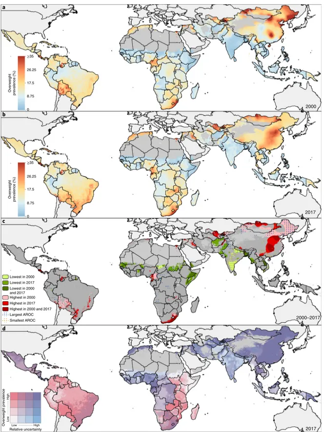
Across LMICs, the prevalence of early childhood overweight increased from 5.2% (95% uncertainty interval, 4.5–5.4%) to 6.0% (4.8–6.1%) in the modeled study period. Between 2000 and 2017, there were noticeable differences in estimated levels by area (Fig. 1a,b). Although levels varied broadly across LMICs, every modeling region had areas with high estimated prevalence in 2017 (Fig. 1b and Extended Data Fig. 1). These included large contiguous areas across most Central American, Caribbean and South American countries and areas with ≥15% estimated prevalence in central Cuba, southern Panama, western Paraguay, scattered throughout several eastern Brazilian states (for example, in Rio Grande do Sul, Minas Gerais, Santa Catarina, Paraná and São Paulo) and Peru’s coastal cities of Tacna, Ilo, Islay, Callao, Trujillo and Lima. In Africa, most countries bordering the Sahel had low overweight prevalence (0–5%); areas with >15% estimated prevalence were concentrated in North Africa throughout Morocco, Algeria, Tunisia, Egypt and select areas of Libya, as well as along South Africa’s southern coast and in pockets in Botswana and Zambia. Large areas in eastern and northern China and throughout Mongolia had an estimated overweight prevalence >15%. Countries in the Oceania region had moderate to high levels, with estimates over 15%, such as in Indonesia’s Jakarta Pusat and Jakarta Barat regencies (in Jakarta Raya; 17.7% (15.3–18.4%)). The North Africa, Central Asia and Southeast Asia regions showed vast differences across nations; for example, Afghanistan, Sudan and Laos had <5% estimated national prevalence, whereas Egypt, Uzbekistan, Morocco, Kyrgyzstan and Thailand had ≥15%. South Asia’s estimated levels ranged from <5% in Bangladesh to ≥10% Bhutan. Estimated prevalence in Karbala city in Karbala, Iraq, increased from 13.6% (12.4–14.1%) in 2000 to 29.3% (22.9–29.1%) in 2017. Thailand’s southern areas experienced large increases in estimated prevalence levels; Sathorn district, Bangkok Metropolis, had 24.1% (20.1–24.8%) overweight in 2000 and 33.9% (27.5–35.5%) in 2017. Areas with the greatest decrease included Churcampa district, Huancavelica, Peru, decreasing from 17.5% (17.4–17.6%) in 2000 to 10.3% (10.2–10.4%) in 2017. Similarly, overweight in Al Gash district, Kassala, Sudan, declined from 14.1% (13.6–14.5%) to 6.1% (5.2–6.2%).
Within-country differences in estimated overweight levels were found in 37 (35.2%) LMICs, including South Africa, Peru and Indonesia, which had twofold differences in estimated prevalence across second administrative units in 2017. South Africa had high estimated national levels (24.9% (23.9–25.2%)); however, the prov-ince of Northern Cape had moderate levels (14.6% (13.6–14.9%)), whereas the southeastern province of Eastern Cape had very high levels (32.7% (30.8–33.9%)). Disparities were further pronounced at the district level. Siyanda (Northern Cape) had 12.5% (11.6–12.9%) prevalence, whereas Ugu (KwaZulu-Natal) had 36.7% (34.0–38.2%). Nearly every modeling region had areas with overweight preva-lence that ranked among the highest decile in 2000, 2017 or both years (Fig. 1c).
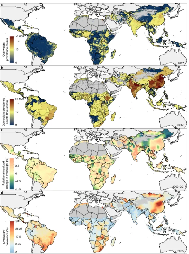
Overall, the number of overweight children under 5 in LMICs also showed a significant increase from 30.0 million (22.8–38.5) to 55.5 million (44.8–67.9) in the study period (Fig. 2a,b). By 2017, 26.2 million (24.1–27.2 million; 36.0%) of those affected lived in eastern Asia, northern Africa or South America. An estimated 8.6% (8.5–9.9%) of first administrative units had fewer than 1,000 overweight children under 5, 47.5% (47.2–49.5%) had 1,000 to <10,000, 43.8% (40.6–44.3%) had 10,000 to <100,000 and just 3.8% (3.7–3.9%) had 100,000 or more. Some areas, such as northern and central parts of Bolivia, experienced large annualized declines such that their ranking among the highest estimated prevalence decile in 2000 no longer applied in 2017. In contrast, a large area in India, south of the Tropic of Cancer, experienced large annualized increases in overweight; its ranking among the lowest prevalence decile in 2000 was not maintained in 2017. All modeled regions had areas that experienced average annualized increases of ≥1% in overweight prevalence (Fig. 2c). Unless current trajectories change, prevalence of overweight will continue to increase to 2025 (Fig. 2d).
Prevalence and trends in child wasting
The estimated prevalence of early childhood wasting decreased over-all across LMICs between 2000–2017, from 8.4% (7.9–9.9%) to 6.4% (4.9–7.9%). The most notable relative reductions were seen across North Africa and in select countries in sub-Saharan African (SSA) regions, Central and Andean America and Southeast Asia regions. In Burkina Faso’s Ganzourgou district, estimated levels declined from 20.2% (19.1–21.3%) in 2000 to 11.6% (10.9–12.1%) in 2017, in Yemen’s Ash Shaikh Outhman district from 25.1% (22.2–26.3%) to 21.3% (18.9–22.2%) and in Sudan’s Al Mahagil district from 31.9% (31.4–32.6%) to 12.2% (10.5–12.9%). Increases in estimated prevalence also occurred, such as in Pakistan’s Makran district (Baluchistan), from 7.4% (6.7–7.6%) to 11.4% (10.4–11.8%).
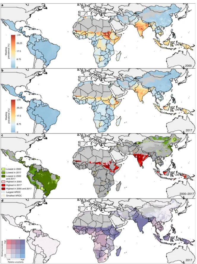
In 2017, there were several instances of contrasting geographic patterns of child wasting compared to those of overweight. Many Central American, Caribbean and South American countries (46%; 11 of 24) affected by overweight (>15% prevalence) met the WHO GNTs for <5% prevalence of wasting across all districts based on estimated prevalence (Fig. 3a,b and Extended Data Fig. 2). Estimated wasting prevalence was ≥15% in 31.9% (850 of 2,661) and ≥20% in 12.9% (342) of second administrative units across Central and South Asian countries, contributing to high prevalence at the national level in India (15.7% (15.4–15.9%)), Pakistan (12.2% (11.8–12.4%)) and Sri Lanka (11.2% (10.5–11.5%)); Afghanistan and Bangladesh maintained high levels (estimated prevalence ≥10%) across many areas. Local-level estimates delineate very high wasting prevalence (≥15%) along the African Sahel from Mauritania to Sudan, in the northeastern Horn of Africa and neighboring countries of Eritrea, Ethiopia, Somalia, Kenya, South Sudan and Yemen, in select areas in Algeria and Egypt, and across Madagascar. In the Middle East, Syria exceeded 15% estimated prevalence throughout most areas and Iraq’s southeastern districts exceeded 10%. Estimated levels of wasting were relatively uniform and low across East Asia, with the exception of a few focal areas exceeding 10% or 20% in central
pockets of east China. Most areas in Southeast Asia and Oceania experienced moderate-to-high estimated wasting levels (~10%), whereas some areas in Indonesia’s southern-most islands in Nusa
Tenggara (Timur state) exceeded 15% prevalence. Meanwhile, some areas in Myanmar, Thailand, northern Laos and Vietnam had very low levels, approaching the WHO GNTs.
a b c d ≥35 26.25 17.5 8.75 0 Overweigh t prevalence (% ) Overweigh t prevalence (% ) ≥35 26.25 17.5 8.75 0 2000 2017 2000–2017 2017 Lowest in 2000 Lowest in 2017 Lowest in 2000 and 2017 Highest in 2000 Highest in 2017 Highest in 2000 and 2017 Largest AROC Smallest AROC Hig h Low High Low Relative uncertainty Overweight prevalenc e
Fig. 1 | Prevalence of overweight children under 5 in LMiCs (2000–2017). a,b, Prevalence of overweight among children under 5 at 5 × 5-km resolution in 2000 (a) and 2017 (b). c, Overlapping population-weighted lowest and highest 10% of grid cells and AROC in overweight from 2000 to 2017. d, Overlapping population-weighted quartiles of overweight and relative 95% uncertainty in 2017. Maps reflect administrative boundaries, land cover, lakes and population; gray colored areas have grid cells classified as ‘barren or sparsely vegetated’ and had fewer than ten people per 1 × 1-km grid cell in 2017 or were not included in this analysis39–45. Maps were generated using ArcGIS Desktop 10.6.
Nature MeDiCiNe | VOL 26 | MAy 2020 | 750–759 | www.nature.com/naturemedicine
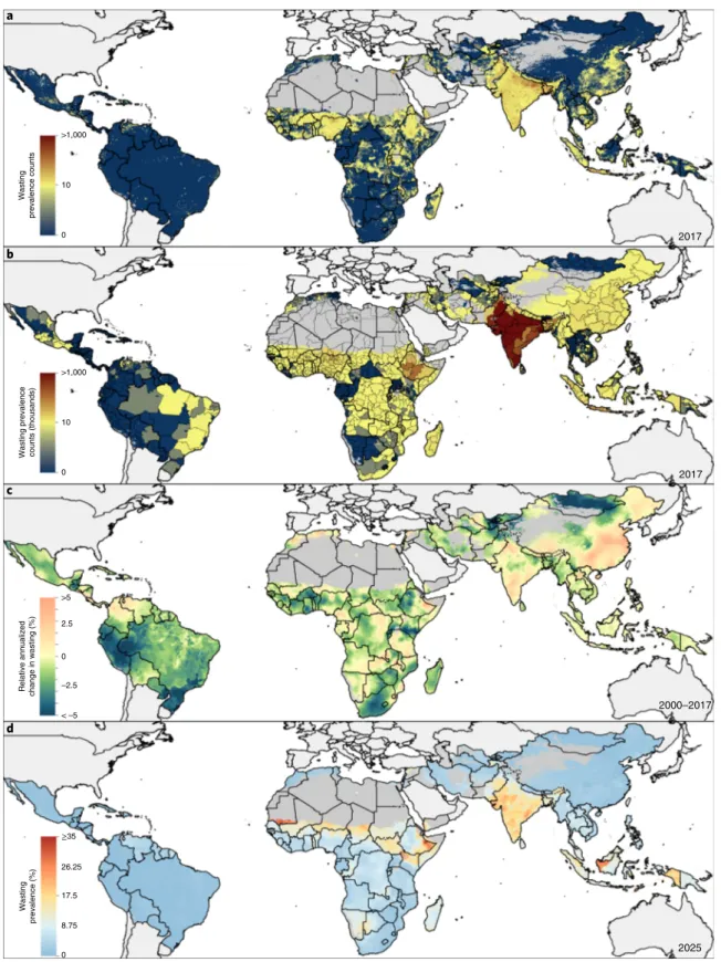
Between 2000 and 2017, the number of children under 5 affected by wasting decreased from 62.3 (55.1–70.8) million to 58.3 (47.6–70.7) million, 28.4% (28.2–28.5) of whom were in Africa and 65.4% (63.6–67.3) in South Asia in 2017 (Fig. 3c,d). Despite maintaining high estimated prevalence in many areas, all regions
in Africa had areas that experienced among the highest rates of annualized declines in 2000–2017; only a few areas in Chad, Sudan, South Sudan, Ethiopia and Kenya were among the highest decile of estimated prevalence levels in both 2000 and 2017 (Fig. 4a,b). Progress differed across and within African countries, with some a b c d 2017 2017 2000–2017 2025 ≥35 17.5 8.75 0 –2.5 0 2.5 >5 < –5 10 0 >1,000 10 0 >1,000 Overweigh t prevalence counts
Overweight prevalence counts (thousands)
Relative annualized change in overweight (% ) Overweigh t prevalence (% ) 26.25
Fig. 2 | Number of overweight children under 5 in LMiCs (2000–2017) and progress toward 2025. a,b, Number of children under 5 affected by overweight at a 5 × 5-km resolution (a) and by first administrative units (b). c, Annualized decrease (AD) in overweight prevalence from 2000 to 2017. d, Grid cell-level predicted overweight prevalence in 2025 based on AD achieved from 2000 to 2017 and projected from 2017. Maps reflect administrative boundaries, land cover, lakes and population; gray colored areas have grid cells classified as ‘barren or sparsely vegetated’ and had fewer than ten people per 1 × 1-km grid cell in 2017 or were not included in this analysis39–45. Maps were generated using ArcGIS Desktop 10.6.
nations, such as Nigeria, Ethiopia and Namibia, experiencing both annualized decreases and increases in wasting within their borders (Fig. 4c). Overall, South America and South SSA demonstrated
the largest annualized declines (≥5%) across most of their areas and regions of Latin America and the Caribbean, the Middle East, South Asia, Southeast Asia and Oceania experienced mostly
Lowest in 2000 Highest in 2000 Largest AROC Smallest AROC Highest in 2017 Lowest in 2000 and 2017 Highest in 2000 and 2017 Lowest in 2017 Wasting prevalence (% ) 8.75 ≥35 0 26.25 17.5 8.75 ≥35 0 26.25 17.5 Wasting prevalenc e Relative uncertainty Low Low High High 2000 2017 2000–2017 2017 Wastin g prevalence (% ) a b c d
Fig. 3 | Prevalence of wasted children under 5 in LMiCs (2000–2017). a–c, Prevalence of moderate and severe wasting among children under 5 at a 5 × 5-km resolution in 2000 (a) and 2017 (b). c, Overlapping population-weighted lowest and highest 10% of grid cells and AROC in wasting from 2000 to 2017. d, Overlapping population-weighted quartiles of wasting and relative 95% uncertainty in 2017. Maps reflect administrative boundaries, land cover, lakes and population; gray colored areas have grid cells classified as ‘barren or sparsely vegetated’ and had fewer than ten people per 1 × 1-km grid cell in 2017 or were not included in this analysis39–45. Maps were generated using ArcGIS Desktop 10.6.
Nature MeDiCiNe | VOL 26 | MAy 2020 | 750–759 | www.nature.com/naturemedicine
annualized increases. Large areas of India and parts of central Pakistan experienced some of the highest prevalence levels through-out the study period, as well as annualized increases. Nearly all South Asian countries had large contiguous areas of stagnation or
annualized increases in wasting; given recent rates of progress, few will meet the WHO GNTs in all their locations by 2025 (Fig. 4d). By 2025, 68 (64.8%) of LMICs are predicted to fail to meet the <5% tar-get nationally, all of which are in Africa, Asia and the Middle East. a b c d Wastin g prevalence (% )
Relative annualized change in wasting (%
)
Wasting prevalence counts (thousands
) Wasting prevalence counts >1,000 10 0 >1,000 10 0 >5 2.5 0 –2.5 < –5 ≥35 26.25 17.5 8.75 0 2025 2000–2017 2017 2017
Fig. 4 | Number of wasted children under 5 in LMiCs (2000–2017) and progress toward 2025. a,b, Number of children under 5 affected by wasting at the 5 × 5-km resolution (a) and by first administrative units (b). c, AD in wasting prevalence from 2000 to 2017. d, Grid cell-level predicted stunting prevalence in 2025 based on AD achieved from 2000 to 2017 and projected from 2017. Maps reflect administrative boundaries, land cover, lakes and population; gray colored areas have grid cells classified as ‘barren or sparsely vegetated’ and had fewer than ten people per 1 × 1-km grid cell in 2017 or were not included in this analysis39–45. Maps were generated using ArcGIS Desktop 10.6.
Based on subnational estimates, 88 (83.8%) and 94 (89.5%) will fail to meet the wasting WHO GNTs in all first and second administra-tive units, respecadministra-tively.
Double burden of wasting and overweight
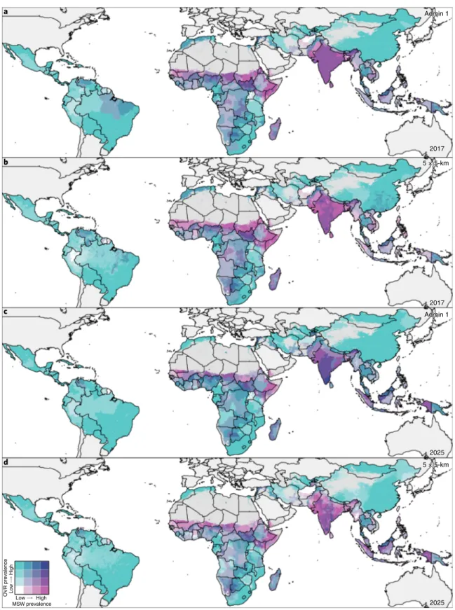
Nearly every modeling region had subnational areas with at least moderate co-occurrence of wasting and overweight (≥5% estimated prevalence of both conditions) in 2017 (Fig. 5 and Extended Data Fig. 3). Exceptions were Central and South America, where Guyana was the only example of moderate DBM (5%–10% of both condi-tions). In Africa, much of the Democratic Republic of the Congo, Cameroon, Republic of Congo, Zambia and southern Botswana demonstrated high DBM (≥10% of both overweight and wasting). Areas in central Morocco reached some of the highest levels of DBM (≥15% overweight, 10–15% wasting), whereas much of the rest of North Africa had high estimated overweight (10–15%) and moderate estimated wasting (5–10%). Locations scattered through-out Iraq, India and in Sthrough-outheast Asia mostly experienced moder-ate wasting (such as Myanmar at 5–10%) or modermoder-ate DBM (such as Indonesia at 5–10%), reaching moderate-to-high DBM levels in select areas (such as central Papua New Guinea and Cambodia at 5–10% overweight, 10–15% wasting; Thailand, 10–15% overweight, 5–10% wasting). Relatively rare in East Asia, DBM was at moder-ate levels at most (5–10% both conditions), such as in provinces in southeastern China. At the national level, 25.7% (27 of 105) LMICs were moderately affected and 5.7% (6 of 105) were highly affected by both overweight and wasting (≥5% and ≥10% prevalence of both conditions, respectively). Subnationally, however, 70.5% (74 of 105) of LMICs had moderately affected districts, 11.4% (12 of 105) had highly affected districts and 2.9% (3 of 105) had districts with very high DBM (≥5%, ≥10% and ≥15% prevalence of both condi-tions, respectively).
Although childhood nutritional status generally improved over 2000–2017, subnational variation in childhood overweight, wasting and DBM was apparent. Declines in wasting and over-weight prevalence in South Africa’s western areas led to a decrease in DBM prevalence, from high levels in Siyanda district in 2005 (10–15% estimated wasting and overweight) to moderate levels in 2017 (5–10% both conditions); overweight remains very high, however, on the southern coast (≥15%). On the basis of annu-alized trends, 25.7% (27 of 105) of LMICs are predicted to have districts with at least moderate DBM by 2025 and 34.3% (36 of 105) are predicted to have high DBM districts (Fig. 5). Between 2000 and 2017, 8.6% (9 of 105) of LMICs had first administrative units that experienced transition from high estimated prevalence of wasting (≥10%) to normal weight (<5% both wasting and over-weight). Nearly one-third, 32.3% (34 of 105) of LMICs had first administrative units that transitioned from normal weight to high overweight and 7.6% (8 of 105) transitioned from high wasting to high DBM.
Discussion
This study provides overweight estimates and combines them with wasting estimates to highlight DBM across LMICs at a fine geospa-tial scale. This enables efficient targeting of local-level interventions to improve nutrition outcomes in vulnerable populations. The fig-ures presented here, as well as our online visualization tools, allow for comparing overweight and wasting levels and trends across and within countries for each year from 2000 to 2017, leveraging the spatially resolved underlying data and covariates to produce detailed spatial estimates across all modeled regions. Our estimates show the global trend in early childhood wasting is declining, but areas with high prevalence and little progress, such as in the Sahel and South Asia, remain. Meanwhile, childhood overweight prevalence has increased, especially in tropical South America and regions in the Middle East, Central Asia and Africa.
Across LMICs, trends in childhood overweight have increased while wasting decreased by different magnitudes from 2000–2017, leading to the emergence of DBM in several areas. As countries experience economic growth, they may undergo nutritional transi-tions wherein the challenges of undernutrition are replaced by those of overweight or the co-occurrence of both conditions4. Overall,
food security has improved across LMICs in the past decade, which has led to increased availability of calories at the population level23.
Although overweight is a reflection of excess calorie intake and reduced energy expenditure, there is a growing recognition that at the root of the rising rates of overweight are complex interactions between societal, environmental, food industry and individual fac-tors, including biological, psychological and economical factors24.
Understanding the factors underpinning these trends is key to pre-dicting how nutrition programs can accelerate amelioration of wast-ing without incurrwast-ing high rates of childhood overweight.
Although we included urbanicity as a covariate in our models, we were unable to reliably stratify our results by urban and rural areas. Urbanization is widely viewed as a key driver of the rise in overweight, but an increase in rural body mass index has recently been recognized as a main driver of the global epidemic of obe-sity in adults25. Such an analysis would thus add important context
to our estimates. Case studies in China, Egypt, India, Mexico, the Philippines and South Africa have demonstrated a consistent trend of increased energy content of diets26. Relatively rural areas in China
have experienced an increase in the intake of animal source foods and edible oils, likely due to the decreasing cost of these products. Further, increased use of motor vehicles and labor-saving technolo-gies in agriculture have caused a decrease in energy expenditure in all these countries. In Brazil, household consumption of high-calorie ultra-processed foods has steadily replaced that of fresh or minimally processed foods27. Nutritious diets consisting of the latter
can help prevent both wasting and stunting, thus work is needed to identify how dietary patterns differ between wasted and over-weight children and the underlying factors causing those differ-ences. Widespread collection and assembly of nutrition data from older children and adults would also contribute to a more complete understanding of longitudinal nutrition patterns.
In addition to tracking progress, child nutrition measurements are important for predicting and averting morbidity and mortal-ity. Wasting is often indicative of short-term weight loss due to food shortages, famine or diseases such as diarrhea28–30 and puts
children at greater risk of succumbing to common infections28.
Childhood overweight is likely to progress into adulthood and is associated with NCDs24, including cardiovascular disease, type
2 diabetes, sleep apnea and cancer31,32. Routine monitoring and
reporting of child nutrition status can highlight trends and act as an early warning for health systems, particularly in the context of epidemiological transitions4.
Although overall spending on development assistance and investments to address malnutrition from government donors have remained steady, those from multilateral institutions have increased since 2013, amounting to US$856 million in overseas development assistance in 2016 (ref. 15). These investments, however, fall short
of the estimated US$3.5 trillion per year that malnutrition costs society, US$500 billion of which is attributable to overweight and obesity33. By focusing on prevention and early action, healthcare
costs can be reduced and human capital increased. One difficulty, however, is addressing the different forms of malnutrition in tan-dem. Multiple forms of malnutrition are the new normal, accord-ing to the GNR15 and Scaling Up Nutrition34,35. Double-duty actions
that could simultaneously combat undernutrition, overweight, obesity, and diet-related NCDs have been proposed to address this problem36–38. Despite progress in identifying such actions, such as
the promotion of breastfeeding, double-duty approaches have not been widely adopted. To better respond to the diverse and rapidly Nature MeDiCiNe | VOL 26 | MAy 2020 | 750–759 | www.nature.com/naturemedicine
evolving nutrition challenges facing LMICs, sustainable and health-promoting food systems are needed to slow the development of DBM. Due to the multiple causality of malnutrition, multisector
collaboration is required, including agriculture, trade and industry, environment, communication and education, all working towards policy and intervention coherence8,24.
OVR prevalence MSW prevalence Low High Low High a b c d 2025 5 × 5-km 2025 2017 Admin 1 5 × 5-km 2017 Admin 1
Fig. 5 | Overlapping population-weighted quartiles of overweight and wasting prevalence in children under 5 across LMiCs in 2017 and 2025. a–d, Prevalence of moderate-to-severe overweight (OVR) and wasting (MSW) among children under 5 years of age in 2017 at the first administrative unit (a) and at a 5 × 5-km resolution (b). c,d, Estimated prevalence of moderate to severe OVR and MSW among children under 5 years of age in 2025 at the first administrative unit (c) and at a 5 × 5-km resolution (d). Quartile cutoffs were 0–5%, ≥5–10%, ≥10–15% and ≥15%. Maps reflect administrative boundaries, land cover, lakes and population; gray colored areas have grid cells classified as ‘barren or sparsely vegetated’ and had fewer than ten people per 1 × 1-km grid cell in 2017 or were not included in these analyses39–45. Maps were generated using ArcGIS Desktop 10.6.
There are several limitations to these analyses, mainly concern-ing the quantity and quality of the underlyconcern-ing data in the models, as shown in our uncertainty maps (Figs. 1f and 2f). Missing or improbable values in the primary data may contribute bias in the estimates and thus we have incorporated covariates to improve the estimates in areas where data are sparse. Additionally, differences in measurement techniques between surveys, scale miscalibration or equipment failure and poor training and standardization of mea-surers may contribute bias. Although our estimates were produced at a high spatial resolution, they were limited to prevalence by area, rather than the co-occurrence of wasting and overweight experi-enced by the same households or individuals. Additional work is required to identify the immediate and basic causes that lead to both wasting and obesity coexisting in the same geographical areas so that appropriate solutions can be identified. Future studies will consider maternal indicators associated with child nutritional out-comes, such as anemia and examine the co-distribution of over-weight and stunting to broaden our assessment. New modeling approaches are currently in development to provide full distribu-tions of height, weight and age, for more complete assessments of DBM using all important indicators of undernutrition.
Commendable gains have been made globally against child malnutrition over the past two decades. Our mapped estimates, however, show that high rates of wasting persist and overweight is increasing among young children in many LMICs. Identifying the causes underlying the presence of wasting or overweight in children living in the same community is necessary to formulate appropriate solutions. The estimates provided by this study can aid in the iden-tification of specific areas where further insight can be gathered and trials of policy interventions administered, ultimately contributing to the UN Decade of Action on Nutrition process of sustained and coherent implementation of policies and programs37.
Online content
Any methods, additional references, Nature Research reporting summaries, source data, extended data, supplementary informa-tion, acknowledgements, peer review information; details of author contributions and competing interests; and statements of data and code availability are available at https://doi.org/10.1038/s41591-020-0807-6.
Received: 25 October 2019; Accepted: 20 February 2020; Published online: 20 April 2020
references
1. Ng, M. et al. Global, regional, and national prevalence of overweight and obesity in children and adults during 1980–2013: a systematic analysis for the global burden of disease study 2013. Lancet 384, 766–781 (2014).
2. Black, R. E. et al. Maternal and child undernutrition and overweight in low-income and middle-income countries. Lancet 382, 427–451 (2013). 3. Black, R. E. et al. Maternal and child undernutrition: global and regional
exposures and health consequences. Lancet 371, 243–260 (2008).
4. World Health Organization. Double burden of malnutrition http://www.who. int/nutrition/double-burden-malnutrition/en/ (2018).
5. de Onis, M., Blössner, M. & Borghi, E. Global prevalence and trends of overweight and obesity among preschool children. Am. J. Clin. Nutr. 92, 1257–1264 (2010).
6. Popkin, B. M., Corvalan, C. & Grummer-Strawn, L. M. Dynamics of the double burden of malnutrition and the changing nutrition reality. Lancet 395, 65–74 (2020).
7. UNICEF, WHO & The World Bank. Joint child malnutrition estimates - levels and trends (2017 edition) https://www.who.int/nutgrowthdb/estimates2016/ en/ (2017)
8. Hawkes, C., Demaio, A. R. & Branca, F. Double-duty actions for ending malnutrition within a decade. Lancet Glob. Health 5, e745–e746 (2017). 9. Cole, T. J., Bellizzi, M. C., Flegal, K. M. & Dietz, W. H. Establishing a
standard definition for child overweight and obesity worldwide: international survey. Brit. Med. J. 320, 1240 (2000).
10. World Health Organization. Training course on child growth assessment
http://www.who.int/childgrowth/training/en/ (2008).
11. de Onis, M. et al. Prevalence thresholds for wasting, overweight and stunting in children under 5 years. Public Health Nutr. 22, 175–179 (2019).
12. United Nations. Goal 2: sustainable development knowledge platform https:// sustainabledevelopment.un.org/sdg2.
13. World Health Organization. Global nutrition targets 2025: childhood overweight policy brief http://www.who.int/nutrition/publications/ globaltargets2025_policybrief_overweight/en/ (2014).
14. World Health Organization. Global nutrition targets 2025: wasting policy brief http://www.who.int/nutrition/publications/globaltargets2025_ policybrief_wasting/en/ (2014).
15. Development Initatives. 2018 Global nutrition report: shining a light to spur action on nutrition https://globalnutritionreport.org/reports/global-nutrition-report-2018/ (2018).
16. United Nations Children’s Fund, World Health Organization & The World Bank. Levels and trends in child malnutrition: key findings of the 2018 edition https://www.who.int/nutgrowthdb/2018-jme-brochure.pdf?ua=1
(2018).
17. World Health Organization. Data: nutrition - joint child malnutrition estimates (2018 edition) http://apps.who.int/gho/tableau-public/tpc-frame. jsp?id=402 (2018)
18. Tzioumis, E., Kay, M. C., Bentley, M. E. & Adair, L. S. Prevalence and trends in the childhood dual burden of malnutrition in low- and middle-income countries, 1990–2012. Public Health Nutr. 19, 1375–1388 (2016).
19. Abarca-Gómez, L. et al. Worldwide trends in body-mass index, underweight, overweight and obesity from 1975 to 2016: a pooled analysis of 2,416 population-based measurement studies in 128.9 million children, adolescents and adults. Lancet 390, 2627–2642 (2017).
20. Humbwavali, J. B., Giugliani, C., Silva, I. C. Mda & Duncan, B. B. Temporal trends in the nutritional status of women and children under five years of age in sub-Saharan African countries: ecological study. Sao Paulo Med. J. Rev.
Paul. Med. 136, 454–463 (2018).
21. Kinyoki, D. K. et al. Mapping child growth failure across low- and middle-income countries. Nature 577, 231–234 (2020).
22. Diggle, P. & Ribeiro, P. J. Model-based Geostatistics (Springer, 2007); https:// doi.org/10.1007/978-0-387-48536-2
23. FAO, IFAD, UNICEF, WFP & WHO. The State of Food Security and Nutrition in the World 2019. Safeguarding Against Economic Slowdowns and Downturns (FAO, 2019).
24. Wells, J. C. et al. The double burden of malnutrition: aetiological pathways and consequences for health. Lancet 395, 75–88 (2020).
25. Bixby, H. et al. Rising rural body-mass index is the main driver of the global obesity epidemic in adults. Nature 569, 260–264 (2019).
26. Food and Agriculture Organization of the United Nations. The double burden of malnutrition. Case studies from six developing countries. FAO Food Nutr.
Pap. 84, 1–334 (2006).
27. Monteiro, C. A., Levy, R. B., Claro, R. M., de Castro, I. R. R. & Cannon, G. Increasing consumption of ultra-processed foods and likely impact on human health: evidence from Brazil. Public Health Nutr. 14, 5–13 (2010).
28. Wang, Y. & Chen, H.-J. in Handbook of Anthropometry (ed. Preedy, V. R.) 29–48 (Springer, 2012).
29. WHO. Physical status: the use and interpretation of anthropometry: report of a WHO Expert Committee http://apps.who.int/iris/bitstream/
handle/10665/37003/WHO_TRS_854.pdf;jsessionid=2FE8F4F177D025F64336 56F4F7577F3F?sequence=1 (1995).
30. Neufeld, L. M. & Osemdar, S. J. M. World nutrition situation: global, regional and country trends in underweight and stunting as indicators of nutrition and health of populations. Internat. Nutr. 78, 11–19 (2013).
31. CDC. Causes and consequences of childhood obesity https://www.cdc.gov/ obesity/childhood/causes.html (2016).
32. Ong, K. K. L., Ahmed, M. L., Emmett, P. M., Preece, M. A. & Dunger, D. B. Association between postnatal catch-up growth and obesity in childhood: prospective cohort study. Brit. Med. J. 320, 967 (2000).
33. Global Panel on Agriculture and Food Systems for Nutrition. The cost of malnutrition: why policy action is urgent https://glopan.org/sites/default/files/ pictures/CostOfMalnutrition.pdf (2016).
34. Scaling Up Nutrition Civil Society Network. SUN Movement Strategy & Roadmap 2016–2020. http://docs.scalingupnutrition.org/wp-content/ uploads/2016/09/SR_20160901_ENG_web_pages.pdf (2016).
35. Scaling Up Nutrition (SUN) Movement: Annual Progress Report 2016.
https://scalingupnutrition.org/wp-content/uploads/2016/11/SUN_Report_ 20161129_web_All.pdf (2016).
36. Hawkes, C. et al. Double-duty actions: seizing programme and policy opportunities to address malnutrition in all its forms. Lancet 395, 142–155 (2020).
37. World Health Organization. United Nations decade of action on nutrition 2016–2025: towards country-specific SMART commitments for action on nutrition http://www.fao.org/3/a-i6130e.pdf (2016).
38. Nugent, R. et al. Economic effects of the double burden of malnutrition.
Lancet 395, 156–165 (2020).
Nature MeDiCiNe | VOL 26 | MAy 2020 | 750–759 | www.nature.com/naturemedicine
39. Global Administrative Areas. GADM database of global administrative areas
http://www.gadm.org (2018).
40. Land Processes Distributed Active Archive Center. Combined MODIS 5.1. MCD12Q1 | LP DAAC: NASA Land Data Products and Services. https:// lpdaac.usgs.gov/products/mcd12q1v006/ (2017).
41. Lehner, B. & Döll, P. Development and validation of a global database of lakes, reservoirs and wetlands. J. Hydrol. 296, 1–22 (2004).
42. World Wildlife Fund. Global lakes and wetlands database, level 3 https:// www.worldwildlife.org/pages/global-lakes-and-wetlands-database (2004). 43. Tatem, A. J. WorldPop, open data for spatial demography. Sci. Data 4,
170004 (2017).
44. WorldPop. WorldPop dataset http://www.worldpop.org.uk/data/get_data/ (2017). 45. GeoNetwork. The Global Administrative Unit Layers (GAUL) http://www.fao.
org/geonetwork/srv/en/main.home (2015).
Publisher’s note Springer Nature remains neutral with regard to jurisdictional claims in
published maps and institutional affiliations.
Open Access This article is licensed under a Creative Commons
Attribution 4.0 International License, which permits use, sharing, adap-tation, distribution and reproduction in any medium or format, as long as you give appropriate credit to the original author(s) and the source, provide a link to the Creative Commons license, and indicate if changes were made. The images or other third party material in this article are included in the article’s Creative Commons license, unless indicated otherwise in a credit line to the material. If material is not included in the article’s Creative Commons license and your intended use is not permitted by statu-tory regulation or exceeds the permitted use, you will need to obtain permission directly from the copyright holder. To view a copy of this license, visit http://creativecommons. org/licenses/by/4.0/.
© The Author(s) 2020
Methods
Overview. Our study follows the Guidelines for Accurate and Transparent Health
Estimates Reporting48 (Supplementary Table 1). The analyses used model-based
geostatistics to generate local-, administrative- and national-level estimates of children under 5 overweight, wasting prevalence and double burden in LMICs over time. Using an ensemble modeling framework that fed into a Bayesian generalized linear mixed-effects model with a correlated space–time random effect and 1,000 draws from an approximate posterior distribution, we generated annual prevalence estimates for overweight and wasting on a 5 × 5-km grid over 105 LMICs from 2000 to 2017 and aggregated these to administrative and national levels (Supplementary Table 2). Countries were selected for inclusion in this study using the socio-demographic index (SDI), a summary measure of development that combines education, fertility and poverty47. Selected countries were in the low,
lower-middle and middle SDI quintiles, with several exceptions (Supplementary Table 2). China, Libya, Malaysia, Panama and Turkmenistan were included despite higher-middle SDIs for geographic continuity with other included countries. Albania, Bosnia-Herzegovina and Moldova were excluded due to geographic discontinuity and lack of available survey data. We did not conduct estimates for the island nations of American Samoa, Federated States of Micronesia, Fiji, Kiribati, Marshall Islands, Samoa, Solomon Islands or Tonga, as no survey data could be sourced.
Data. Surveys and child anthropometry data. We extracted individual-level height,
weight and age data for children under 5 from household survey series including the Demographic and Health Surveys, Multiple Indicator Cluster Surveys, Living Standards Measurement Study and Core Welfare Indicators Questionnaire, among other country-specific child health and nutrition surveys49–52 (Supplementary
Tables 3 and 4). Included in our models were 420 georeferenced household surveys representing over 3 million children under 5. Each individual child record was associated with a cluster, a group of neighboring households or a ‘village’ that acted as a primary sampling unit. Approximately 185 surveys with height, weight and age data included geographic coordinates or precise place names for each cluster within that survey. In the absence of geographic coordinates for each cluster, we assigned data to the smallest available administrative areal unit in the survey (polygon) while accounting for the survey sample design (15,781 survey polygons for overweight and wasting)53,54. Boundary information for these
administrative units was obtained as shapefiles either directly from the surveys or by matching to shapefiles in the Global Administrative Unit Layers55 database or
the Database of Global Administrative Areas56. In select cases, shapefiles provided
by the survey administrator were used or custom shapefiles were created based on survey documentation. These areal data were resampled to point locations using a population-weighted sampling approach over the relevant areal unit with the number of locations set proportionally to the number of grid cells in the area and the total weights of all the resampled points summing to one43.
Select data sources were excluded for the following reasons: missing survey weights for areal data, missing sex or age variable, incomplete sampling (for example, only children ages 0–3 years measured) or untrustworthy data (as determined by the survey administrator or by inspection). Details on the survey data excluded for each country can be found in Supplementary Table 5. Data extraction and processing methods have been described previously21.
Child anthropometry. Using height, weight, age and sex data for each individual,
WHZs were calculated using the age-, sex- and indicator-specific lambda-mu-sigma values from the 2006 WHO Child Growth Standards10,57. The
lambda-mu-sigma methodology allows for Gaussian z score calculations and comparisons to be applied to skewed, non-Gaussian distributions58. A child was classified as
overweight or wasted if their weight-for-height/length was more than two s.d. (z scores) above or below the WHO growth reference population, respectively59.
These individual-level data observations were then collapsed to cluster-level totals for the number of children sampled and total number of children under 5 affected by overweight and the total number of children who are wasted out of the children who were not overweight.
Temporal resolution. We estimated prevalence of overweight and wasting annually
from 2000 to 2017 using a model that allowed us to account for data points measured across survey years, and as such, allows us to predict at monthly or finer temporal resolutions. We were limited, however, both computationally and by the temporal resolution of covariates (Supplementary Table 6) and thus produced only annual estimates.
Seasonality adjustment. WHZs were used to calculate individual child wasting
status. As a data preprocessing step, we performed a seasonality adjustment on individual-level child weights in order to account for differences in observed child weight that may have been due to food scarcity during the month in which the survey was conducted. To adjust weight measurements, we fitted a model for each region with a 12-month seasonal spline, a country-level fixed effect and a smooth spline over the duration of our data collection using the mgcv package in R and the following formula:
WHZ sccðmonthÞ þ stpð Þ þ as:factor countryt ð Þ:
I
Month is the integer-valued month of the year (1, …, 12), t is the time of the interview in integer months since the earliest observation of any child in the dataset and country is a factor variable representing the country where the observation was recorded. We modeled the periodic component on months using 12 cyclic cubic (cc) regression splines basis functions and we accounted for a smooth longer time temporal trend using four thin-plate (tp) splines. The country effects and the long-term temporal spline were included only to avoid confounding during fitting of the seasonal spline fit and neither country effects nor the long-term trend was used in the seasonal adjustment. We then adjusted all observations to account for the difference in the seasonal period between the month of the interview and an average day of the year as determined by which days aligned with the mean of the periodic spline.
Spatial covariates. In order to leverage strength from locations with observations
to the entire spatial–temporal domain, we compiled several 5 × 5-km raster layers of putative socioeconomic and environmental correlates of malnutrition in the 105 LMICs (Supplementary Table 6). These covariates were selected based on their potential to be predictive for overweight and wasting, according to literature review and plausible hypothesis as to their influence. Acquisition of temporally dynamic datasets, where possible, was prioritized to best match our observations and thus predict the changing dynamics of the two indicators. Of the 12 covariates included, 6 were temporally dynamic and were reformatted as a synoptic mean over each estimation period or as a mid-period year estimate. These included average daily mean rainfall (precipitation), educational attainment in women of reproductive age (15–49 years old), enhanced vegetation index, fertility, urbanicity and population. The remaining six covariate layers were static throughout the study period and were applied uniformly across all modeling years; these covariates included growing season length, irrigation, nutritional yield for vitamin A, nutritional yield for protein, nutritional yield for iron and travel time to nearest settlement >50,000 inhabitants.
To select covariates and capture possible nonlinear effects and complex interactions between them, an ensemble covariate modeling method was implemented60. For each region, three submodels were fitted to our dataset, using
all of our covariate data as explanatory predictors: generalized additive models, boosted regression trees and lasso regression. Each submodel was fitted using fivefold cross-validation to avoid overfitting and the out-of-sample predictions from across the five holdouts were compiled into a single comprehensive set of out-of-sample predictions from that model. Additionally, the same submodels were also run using 100% of the data and a full set of in-sample predictions were created. The three sets of out-of-sample submodel predictions were fed into the full geostatistical model as the explanatory covariates when performing the model fitting. The in-sample predictions from the submodels were used as covariates when generating predictions using the fitted full geostatistical model. A recent study has shown that this ensemble approach can improve predictive validity by up to 25% over an individual model60.
Analysis. Geostatistical model. In this study, wasting was defined as the proportion
of children under 5 below negative 2 WHZ (<−2 WHZ); normal category, the proportion of children under 5 between negative 2 and positive 2 WHZ z score (>−2 and <2 WHZ); and overweight was defined as the proportion of children under 5 above positive 2 WHZ z score (>2 WHZ) as defined in the WHO growth reference population59. To model the full distribution of possible indicators of
nutritional status in WHZ (wasting (<−2 WHZ), normal (>−2 and <2 WHZ) and overweight (>2 WHZ)), we used an ordinal modeling approach61,62 to estimate the
relative proportion of each indicator. A similar modeling approach was used to estimate vaccine coverage in Africa63.
We used a continuation ratio model to estimate the prevalence of three categories: wasting, normal weight and overweight. We first modeled the proportion of wasting children within a Bayesian hierarchical framework using logistic regression with a spatially and temporally explicit generalized linear mixed-effects model. Second, we modeled the proportion of the children that were overweight conditioned on not being wasted using the same Bayesian modeling framework. The estimates from the second conditional model were then combined with the wasting estimates to compute the proportion of overweight children in the full distribution.
At each cluster, j, where j = 1, 2, …n, and time t, where t = 2000, 2001, …2017, the prevalence of wasting was modeled using the observed number of children in cluster
d, who were found to be wasted as a binomial count data Cd among a sample size Nd.
Cdjpi dð Þ;t dð Þ;Nd Binomial p�i dð Þ;t dð Þ;Nd8 observe clusters d logit p� i;t
¼ β0þ Xi;tβ þ Zi;tþ ϵctrðiÞþ ϵi;tþ Zi;t8i 2 spatial domain 8 t 2 time domain
P3 h¼1
βh¼ 1
ϵctr iid Normal 0; γð 2Þ ϵi;t iid Normal 0; σð 2Þ
Z GPð0; Σspace ΣtimeÞ Σspace¼ ω2 Γ νð Þ2v�1´ κDð Þ ν´ K νð ÞκD Σtime j;k ¼ ρjk�jj
For indices d, i and t, *(index) is the value of * at the index. The annual prevalence of wasting, pi,t, in cluster i, in time t, was modeled as a linear
combination of the three submodels, (generalized additive models, boosted regression trees and lasso regression), rasterized covariate values, Xi,t, a correlated
spatiotemporal random effect term Zi,t, country random effects ϵctrðiÞ
I , with one
unstructured country random effect fitted for each country in the modeling region and all ϵctr
I sharing a common variance parameter, γ
2, and an independent nugget random effect ϵi;t
I, with variance parameter, σ
2. Coefficients β
h in the
three submodels h = 1, 2, 3 represent their respective predictive weighting in the logit link, while the joint error term Zi,t accounts for residual spatiotemporal
autocorrelation between individual data points that remain after accounting for the predictive effect of the submodel covariates, the country-level random effect
ϵctrðiÞ
I
and the nugget, ϵi;t
I. The residuals Zi,t, were modeled as a three-dimensional
Gaussian process in space–time centered at zero and with a covariance matrix constructed from a Kronecker product of spatial and temporal covariance kernels. The spatial covariance, Σspace, was modeled using an isotropic and stationary Matérn function64 and temporal covariance, Σtime, as an annual autoregressive (AR1) function over the 18 years represented in the model. In the stationary Matérn function, Γ is the gamma function, Kv is the modified Bessel function of
order v > 0, κ > 0 is a scaling parameter, D denotes the Euclidean distance and ω2 is the marginal variance. The scaling parameter, κ, is defined to be κ ¼pffiffiffiffiffi8v=δ
I ,
where δ is a range parameter (about the distance where the covariance function
approaches 0.1) and v is a scaling constant, which is set to 2 rather than fitted from the data. The number of rows and the number of columns of the spatial Matérn covariance matrix are both equal to the number of spatial mesh points for a given modeling region. The number of rows and the number of columns of the spatial Matérn covariance matrix are both equal to the number of spatial mesh points for a given modeling region. In the AR1 function, ρ is the autocorrelation function
and k and j are points in the time series where |k−j| defines the lag. The number of rows and the number of columns of the AR1 covariance matrix are both equal to the number of temporal mesh points (18). The number of rows and the number of columns of the space–time covariance matrix, Σspace⊗Σtime, for a given modeling region are both equal to the number of spatial mesh points × the number of temporal mesh points.
This approach leverages the residual correlation structure to more accurately predict prevalence estimates for locations with no data, while also propagating the dependence in the data through to uncertainty estimates65. The
posterior distributions were fitted using computationally efficient and accurate approximations in R-INLA66,67 (integrated nested Laplace approximation) with the
stochastic partial differential equations68 approximation to the Gaussian process
residuals using R project v.3.5.1. The stochastic partial differential equations approach using INLA has been demonstrated elsewhere, including the estimation of health indicators, particulate air matter and population age structure69–71.
Uncertainty intervals were generated from 1,000 draws (statistically plausible candidate maps)72 created from the posterior-estimated distributions of
modeled parameters.
Post estimation. To transform grid cell-level estimates into a range of information
useful to a wide constituency of potential users, estimates were aggregated at first and second administrative units specific to each country and at national levels73. Although the models can predict all locations covered by available raster
covariates, all final model outputs for which land cover was classified as ‘barren or sparsely vegetated’ on the basis of Moderate Resolution Imaging Spectroradiometer (MODIS) satellite data (2013) were masked74. Areas where the total population
density was less than ten individuals per 1 × 1-km grid cell in 2015 were also masked in the final outputs.
Model validation. Models were validated using spatially stratified fivefold
out-of-sample cross-validation. In order to offer a more stringent analysis by accounting for some of the spatial correlation in the data, holdout folds were created by combining sets of all data falling with first administrative level areas. Validation was performed by calculating bias (mean error), variance (root-mean-square error), 95% data coverage within prediction intervals and correlation between observed data and predictions. All validation metrics were calculated on the out-of-sample predictions from the fivefold cross-validation. All validation procedures and corresponding results are provided in Supplementary Tables 7–18.
Projections. To compare our estimated rates of improvement in overweight
and wasting prevalence over the last 18 years with the improvements needed between 2017 and 2025 to meet WHO GNTs, we performed a simple projection using estimated AROC applied to the final year of our estimates. Both AROC and projections were calculated at the draw-level to obtain the uncertainty of the estimates.
For each indicator i, we calculated AROC at each grid cell (m) by calculating the AROC between each pair of adjacent years t:
AROCu;m;t¼ logit
pu;m;t
pu;m;t�1
We then calculated a weighted AROC for each indicator by taking a weighted average across the years, where more recent AROCs were given more weight in the average. We defined the weights to be:
Wt¼ ðt � 2000 þ 1γÞ;
where γ may be chosen to give varying amounts of weight across the years. For each
indicator, we then calculated the average AROC to be: AROCu;m¼
X2017 2001
Wt´ AROCu;m;t
!
Finally, we calculated the projections (Proj) by applying the AROC in our 2017 mean prevalence estimates to produce estimates in 8 years from 2017 to 2025.
Proju;m;2025¼ logit�1logit p
u;m;2017
þ AROCu;m´ 8
:
This projection scheme is analogous to the methods used in the Global Burden of Disease 2017 study47 for measurement of progress and projected attainment
of health-related Sustainable Development Goals. Our projections are based on the assumption that areas will sustain the current AROC, and the precision of the AROC estimates is dependent on the level of uncertainty emanating from the estimation of annual prevalence.
Priors. The following priors were used for our overweight and wasting models: β0 N μ ¼ 0; σð 2¼ 32Þ;
β iidN μ ¼ 1
no: ensemble models; σ2¼ 32
; log 1þρ1�ρ Nðμ ¼ 4; σ2¼ 1:22Þ; log 1 σ2 nug loggamma α ¼ 1; γ ¼ 5 ´ 10ð �5Þ: log 1 σ2 country loggamma α ¼ 1; γ ¼ 5 ´ 10ð �5Þ: θ1¼ log σ2k Nðμθ1; σ 2 θ1Þ θ2¼ log κð Þ Nðμθ2; σ2θ2Þ
Given that our covariates used in INLA (the predicted outputs from the ensemble models) should be on the same scale as our predictive target, we believe that the intercept in our model should be close to zero and that the regression coefficients should sum to 1. As such, we chose the prior for our intercept to be N(0,σ2= 32) and the prior for the fixed-effect coefficients to be
N 1
no: ensemble models; σ2¼ 32
I . The prior on the temporal correlation parameter,
ρ, was chosen to be mean zero, showing no prior preference for either positive or
negative autocorrelation structure and with a distribution wide enough such that within three s.d. of the mean, the prior includes values of ρ ranging from −0.95
to 0.95. The priors on the random effect variances were chosen to be relatively loose given that we believe our fixed-effects covariates should be well correlated with our outcome of interest, which might suggest relatively small random effects values. At the same time, we wanted to avoid using a prior that was so diffuse as to actually put high prior weight on large random effect variances. For stability, we used the uncorrelated multivariate normal priors that INLA automatically determines (based on the finite elements mesh) for the log-transformed spatial hyperparameters κ and τ. In our parameterization, we represent α and γ in the log
gamma distribution as shape and inverse-scale, respectively.
Prior sensitivity analysis. Sensitivity analysis was undertaken to assess the impact
of the hyper-priors for the nugget, country random effects, and space–time correlation. We considered two different sets of priors related to the nugget and country random effects and three set related to space–time correlation, resulting in six different combinations of hyper-priors as outlined below.
Model 1: In this model, we used the default hyper-priors in INLA75 (for both
nugget and country random effects. The hyper-prior for the AR1 rho, ρ, was
retained as shown below. log 1 σ2 nugget loggamma α ¼ 1; γ ¼ 5 ´ 10ð �5Þand log 1 σ2 counry loggamma α ¼ 1; γ ¼ 5 ´ 10ð �5Þ: log 1þρ 1�ρ Normal ðμ ¼ 4; σ2¼ 1:22Þ
Model 2: The hyper-priors for nugget were changed as indicated below, where hyper-priors for country random effect were the default hyper-priors in INLA. The hyper-priors for the AR1 rho, ρ, were retained the same as model 1.
log 1 σ2 nugget loggamma α ¼ 1; γ ¼ 2ð Þ and log 1 σ2 counry loggamma α ¼ 1; γ ¼ 5 ´ 10ð �5Þ: log 1þρ 1�ρ Normal ðμ ¼ 4; σ2¼ 1:22Þ
Model 3: In this model the hyper-priors for country random effects and nugget were exchanged, where hyper-priors for nugget were the default hyper-priors in INLA. The hyper-priors for the AR1 rho, ρ, were retained the same as model 1.
log 1 σ2 nug loggamma α ¼ 1; γ ¼ 5 ´ 10ð �5Þ and log 1 σ2 counry loggamma α ¼ 1; γ ¼ 2ð Þ: log 1þρ1�ρ Normal ðμ ¼ 4; σ2¼ 1:22Þ
Model 4: In this model, we used the default hyper-priors in INLA for less informative nugget and country random effects. The hyper-priors for the AR1 rho,
ρ, were changed. log 1 σ2 nugget loggamma α ¼ 1; γ ¼ 5 ´ 10ð �5Þ and log 1 σ2 counry loggamma α ¼ 1; γ ¼ 5 ´ 10ð �5Þ: log 1þρ 1�ρ Normal ðμ ¼ 0; σ2¼ 1:22Þ
Model 5: In this model, we used the default hyper-priors in INLA for both nugget and country random effects. The hyper-priors for the AR1 rho, ρ, were the
default in INLA. log 1 σ2 nugget loggamma α ¼ 1; γ ¼ 5 ´ 10ð �5Þ and log 1 σ2 counry loggamma α ¼ 1; γ ¼ 5 ´ 10ð �5Þ: log 1þρ 1�ρ Normal ðμ ¼ 0; σ2¼ 2:582Þ
The predicted estimates for all models with different sets of hyper-priors were highly correlated at the grid-cell level and yielded low mean absolute differences (Supplementary Table 7). We ultimately selected the less informative priors for nugget and country random effects as they are default priors in the INLA package and have been applied widely76,77 and selected a more stringent parameterization of
our space–time correlation, as indicated in model 1.
Mesh construction. We constructed the finite elements mesh for the stochastic
partial differential equation approximation to the Gaussian process regression using a simplified polygon boundary (in which coastlines and complex boundaries were smoothed) for each of the regions within our model. We set the inner mesh triangle maximum edge length (the mesh size for areas over land) to be 0.75 degrees and the buffer maximum edge length (the mesh size for areas over the ocean) to be 5 degrees. An example finite elements mesh constructed for Eastern SSA mesh is described by Kinyoki et al.21.
Reporting Summary. Further information on research design is available in the
Nature Research Reporting Summary linked to this article.
Data availability
Our study follows the Guidelines for Accurate and Transparent Health Estimates Reporting48 (Supplementary Table 1). The findings of this study are supported by
data available in public online repositories, data publicly available upon request of the data provider and data not publicly available due to restrictions by the data provider. Nonpublicly available data were used under license for the current study but may be available from the authors upon reasonable request and with permission of the data provider. Details of data sources and availability can be found in Supplementary Tables 2–5. The full output of the analyses are publicly available in the Global Health Data Exchange (http://ghdx.healthdata.org/record/ ihme-data/lmic-double-burden-of-malnutrition-geospatial-estimates-2000-2017) and can further be explored via customized data visualization tools (https://vizhub. healthdata.org/lbd/dbm.). Administrative boundaries were retrieved from the Database of Global Administrative Areas39. Land cover was retrieved from the
online Data Pool, courtesy of the NASA EOSDIS Land Processes Distributed Active Archive Center, USGS/Earth Resources Observation and Science Center, Sioux Falls, South Dakota40. Lakes were retrieved from the Global Lakes and
Wetlands Database, courtesy of the World Wildlife Fund and the Center for Environmental Systems Research, University of Kassel41,42. Populations were
retrieved from WorldPop43,44.
Code availability
All code used for these analyses is publicly available online at http://ghdx. healthdata.org/record/ihme-data/lmic-double-burden-of-malnutrition-geospatial-estimates-2000-2017 and at http://github.com/ihmeuw/lbd/tree/dbm-lmic-2020.
references
47. Dicker, D. et al. Global, regional, and national age-sex-specific mortality and life expectancy, 1950–2017: a systematic analysis for the global burden of disease study 2017. Lancet 392, 1684–1735 (2018).
48. Stevens, G. A. et al. Guidelines for accurate and transparent health estimates reporting: the GATHER statement. PLoS Med. 13, e1002056 (2016).
49. USAID. Demographic and health surveys (DHS) http://dhsprogram.com/. 50. UNICEF. Multiple indicator cluster surveys (MICS) http://mics.unicef.org. 51. World Bank Group. Living standards measurement survey (LSMS) http://
go.worldbank.org/UK1ETMHBN0.
52. World Bank Group. Core welfare indicators questionnaire survey (CWIQ)
http://ghdx.healthdata.org/series/core-welfare-indicators-questionnaire-survey-cwiq.
53. Lumley, T. in Complex Surveys: A Guide to Analysis Using R. (Wiley, 2010). 54. Lumley, T. Analysis of complex survey samples. J. Stat. Softw. 9,
1–19 (2004).
55. FAO. The global administrative unit layers (GAUL): technical aspects http:// www.fao.org/geonetwork/srv/en/main.home.
56. Global Administrative Areas (GADM). GADM database of global administrative areas http://www.gadm.org.
57. WHO Multicentre Growth Reference Study Group. WHO child growth standards based on length/height, weight and age. Acta Paediatr. Suppl, 450, 76–85 (2006).
58. Indrayan, A. Demystifying LMS and BCPE methods of centile estimation for growth and other health parameters. Indian Pediatr. 51, 37–43 (2014).
59. WHO Multicentre Growth Reference Study Group. WHO child growth standards based on length/height, weight and age. Acta Paediatr 95, 76–85 (2006).
60. Bhatt, S. et al. Improved prediction accuracy for disease risk mapping using Gaussian process stacked generalization. J. R. Soc. Interface 14, 20170520 (2017).
61. Fienberg, S. E. The Analysis of Cross-Classified Categorical Data (Springer, 2007); https://doi.org/10.1007/978-0-387-72825-4
62. Ananth, C. V. & Kleinbaum, D. G. Regression models for ordinal responses: a review of methods and applications. Int. J. Epidemiol. 26, 1323–1333 (1997). 63. Mosser, J. F. et al. Mapping diphtheria-pertussis-tetanus vaccine coverage in
Africa, 2000–2016: a spatial and temporal modelling study. Lancet 393, 1843–1855 (2019).
64. Stein, M. L. Interpolation of Spatial Data (Springer, 1999).
65. Diggle, Peter J. & Ribeiro, Paulo J. Model-based Geostatistics (Springer, 2007);
https://doi.org/10.1007/978-0-387-48536-2.
66. Rue, H., Martino, S. & Chopin, N. Approximate Bayesian inference for latent Gaussian models by using integrated nested Laplace approximations.
J. R. Stat. Soc. Ser. B Stat. Methodol. 71, 319–392 (2009).
67. Martins, T. G., Simpson, D., Lindgren, F. & Rue, H. Bayesian computing with INLA: new features. Comput. Stat. Data Anal. 67, 68–83 (2013).
68. Lindgren, F., Rue, H. & Lindström, J. An explicit link between
Gaussian fields and Gaussian Markov random fields: the stochastic partial differential equation approach. J. R. Stat. Soc. Ser. B Stat. Methodol.73, 423–498 (2011).
69. Golding, N. et al. Mapping under-5 and neonatal mortality in Africa, 2000–15: a baseline analysis for the sustainable development goals. Lancet
390, 2171–2182 (2017).
70. Osgood-Zimmerman, A. et al. Mapping child growth failure in Africa between 2000 and 2015. Nature 555, 41–47 (2018).
71. Alegana, V. A. et al. Fine resolution mapping of population age-structures for health and development applications. J. R. Soc. Interface 12,
20150073–20150073 (2015).
72. Patil, A. P., Gething, P. W., Piel, F. B. & Hay, S. I. Bayesian geostatistics in health cartography: the perspective of malaria. Trends Parasitol. 27, 246–253 (2011).
73. Gething, P. W., Patil, A. P. & Hay, S. I. Quantifying aggregated uncertainty in
Plasmodium falciparum malaria prevalence and populations at risk via
efficient space-time geostatistical joint simulation. PLoS Comput. Biol. 6, e1000724 (2010).
74. Scharlemann, J. P. W. et al. Global data for ecology and epidemiology: a novel algorithm for temporal Fourier processing MODIS data. PLoS ONE 3, e1408 (2008).
75. Blangiardo, M. & Cameletti, M. in Spatial and Spatio‐temporal Bayesian
Models with R‐INLA 235–258 (John Wiley & Sons, 2015).
76. Cameletti, M., Lindgren, F., Simpson, D. & Rue, H. Spatio-temporal modeling of particulate matter concentration through the SPDE approach.
AStA Adv. Stat. Anal. 97, 109–131 (2013).
77. Blangiardo, M., Cameletti, M., Baio, G. & Rue, Havard Spatial and spatio-temporal models with R-INLA. Spat. Spatio-Temporal Epidemiol. 7, 39–55 (2013).
acknowledgements
This work was primarily supported by grant OPP1132415 from the Bill & Melinda Gates Foundation awarded to S.I.H. The corresponding author had full access to data in the study and had final responsibility for the decision to submit the study for publication.