Do global oil prices drive domestic food prices?

(1)

Master

's thesis • 30 credits

Agricultural programme – Economics and Management

Do Global Oil Prices Drive Domestic Food

Prices?

-

evidence from the Middle East countries

(2)

Swedish University of Agricultural Sciences

Faculty of Natural Resources and Agricultural Sciences

Do Global Oil Prices Drive Domestic Food Prices? -evidence

from the Middle East countries

Madina Alieva

Supervisor:

Examiner:

Assem Abu Hatab, Swedish University of Agricultural Sciences, Department of Economics

Jens Rommel, Swedish University of Agricultural Sciences, Department of Economics Credits: Level: Course title: Course code: Programme/Education: 30 hec A2E

Master thesis in Economics EX0907

Agricultural programme

– Economics and Management 120,0 hp

Course coordinating department:Department of Economics Place of publication: Year of publication: Name of Series: Part number: ISSN: Online publication: Key words: Uppsala 2019

Degree project/SLU, Department of Economics 1231

1401-4084

http://stud.epsilon.slu.se

food price, crude oil price, cointegration, VECM, Middle East

(3)

Abstract

This study investigates the dynamic relationship between global oil prices and domestic food prices across 11 countries of the Middle East. Using monthly data covering the period from January 2010 to October 2018, the study employs long-run cointegration tests, vector error correction model (VECM) and vector autoregression (VAR) model to examine the effect of global oil prices on domestic food prices in a sample of Middle East countries.

The results of panel cointegration tests revealed that there is a long-run relationship between global oil and domestic food prices. Panel VECM along with Granger causality tests showed that in the short-run there is no significant causality running from oil to food prices, while in the long-run global oil prices positively affect domestic food prices.

At the country level, the empirical findings provide inconclusive evidence on the impact of global oil prices on domestic food prices in the region. While Johansen cointegration tests showed long-run relationship between oil and food prices for Bahrain, Egypt and Kuwait, VECM indicated long-run positive and significant oil price transmission only for Bahrain and Egypt. The short-run parameters obtained through VAR and Granger causality tests revealed positive and significant oil price causality on domestic food prices for Bahrain and Saudi Arabia with lesser impact in Lebanon, Qatar and Turkey.

The findings provide some policy implications, such as reconsideration of current food subsidies and price controls, tackling domestic issues related to logistics and infrastructure by improving transportation system and supply chains, as well as maintaining trade diversification within and outside the Middle East region.

The paper contributes to the literature on dynamics of commodity prices and global-to-local price transmission in the as understanding of the relationship and the ability to make a prognosis is of a significant importance for policymakers when formulating future fuel and food policies, and for researchers and economic agents when analysing price forecasts and strategies.

(4)

(5)

List of figures

Figure 1. The relationship between global food prices and oil prices. ... 1

Figure 2. The empirical modelling framework. ... 13

List of tables

Table 1. Descriptive statistics of the time series variables. ... 20

Table 2. Results for panel unit root tests. ... 21

Table 3. Johansen Fisher panel cointegration test results. ... 22

Table 4. VECM long-run parameters. ... 23

Table 5. VECM short-run parameters. ... 23

Table 6. Granger causality test results. ... 24

Table 7. Unit root tests results. ... 25

Table 8. Johansen cointegration tests results. ... 26

Table 9. VECM short-run parameters. ... 27

Table 10. VECM long-run parameters. ... 28

Table 11. VAR short-run parameters. ... 29

(7)

Abbreviations

ADF Augmented Dickey-Fuller test

ARDL Autoregressive Distributed Lag model

ARMA Autoregressive Moving-Average model

CPI Consumer Price Index

ECT Error Correction Term

FAO United Nations Food and Agriculture Organization

FAOSTAT Food and Agriculture Organization Statistical Database

FCPI Consumer Price Index corresponding to food

GCC Gulf Cooperation Council

IFPRI International Food Policy Research Institute

IFS International Financial Statistics from International Monetary Fund database

LLC Levin, Lin, and Chu panel unit root test

PP Phillips-Perron unit root test

UAE United Arab Emirates

VAR Vector Autoregression

VECM Vector Error Correction Model

(8)

(9)

1 Introduction

Do global oil prices cause higher food prices? And if so, does the impact differ across countries? The present thesis attempts to answer these questions by investigating the impact of oil price movements on domestic food prices in the Middle East countries.

Over the past two decades, agricultural commodity prices have become increasingly volatile in developing countries (Gilbert, 2010; Ortiz, Chai & Cummins, 2011; Bakucs & Fertő, 2013). A number of studies have showed that such volatile food prices have coincided with fluctuations in international oil prices (Dillon et al., 2014; Tadesse et al., 2014; Wang, Wu & Yang, 2014). As shown in Figure 1, food and crude oil price indices have been moving hand-in-hand during the period 2000-2018. Starting from 2003 oil prices experienced sharp rises that continued until the middle of 2008. This has been attributed to a number of reasons which include the increased demand for oil in the United States and emerging countries such as China and India, the weakening of the US dollar, and the decreased oil production due to the occupation of Iraq (Chen, Kuo & Chen, 2010; Belke & Dreger, 2015).

Figure 1. The relationship between global food prices and oil prices.

Source: Own calculations based on data from The World Bank Commodity Price Data, 2018.

Skyrocketing prices of agricultural commodities, almost as oil price increases starting from 2004 resumed the urgency of addressing food security issues due to raised fears among policy makers about global food shortage and inflationary pressures (Olayungbo & Hassan, 2016). According to the World Bank, the global agricultural commodity prices increased by more than

0 50 100 150 200 250 300 350 00 02 04 06 08 10 12 14 16 Food Grains

Maize Oils & Meals Other Food Crude Oil

(10)

80% over the period of 2005 to 2008 (Holt-Giménez & Peabody, 2008). This spike in food prices put significant pressure on developing food-importing countries that had to manage the surge of food and oil prices in a fragile macroeconomic environment.

The explanations given to the food price increases vary and researches find it hard to agree on a single factor. There are various interdependent structural and supply- and demand-side factor that caused the price spikes (Tadesse et al., 2014). The supply-side factors include, but no limited to, global cereal productivity decrease, insufficient global grain reserves, trade restrictions or bans on export of key agricultural commodities, diversion of agricultural land for bioenergy production (Obadi & Korček, 2014). The rapidly increasing global population, shifts in food consumption patterns and urbanization in developing and emerging countries present pressures on the demand side.

While the global economic and financial crises caused a decline of international demand for commodities, negatively affecting oil and food prices, they recovered and surged again in 2010-2011 before going down from 2012. At present, the aggregate food price index is higher than the levels observed in mid-2000s and prices of certain agricultural commodities remain to be high (World Bank, 2014). Indeed, extreme price fluctuations of agricultural commodities not only affect the food security of the poor segments of population in developing countries, but they also affect the economic growth and social stability (Dillon et al., 2015; Olayungbo & Hassan, 2016; Ceballos et al., 2017).

Given that worldwide surge in food prices followed increases in crude oil prices, researchers raised a concern that oil and food prices are more closely linked (Baumeister & Kilian, 2014). In this context, the academic literature points out that oil price spikes among other factors, affect food prices in the developing countries due to a number of reasons. Ahmadi et al. (2015) point out three main linkage channels between oil and agricultural commodity prices. First, due to the increase in oil prices caused by the improved international economic activity, the demand for food also increases, as higher level of income in emerging economies affects the consumption pattern of food. Hochman et al. (2012) and Baumeister and Peersman (2013) emphasize the importance of such link through which oil prices influence food prices. Second, the increase in a crude oil price pushes crop production costs up and consequently the supply curve of food commodities to the left, and as a result price of food commodities rises (Wang, Wu & Yang, 2014; Ahmadi, Bashiri Behmiri & Manera, 2016; Chiu et al., 2016). Therefore, it is argued that rising oil prices result in increase of agricultural commodity prices through cost-push effects by increasing production costs as farm inputs, such as inorganic fertilizers and fuel

(11)

for equipment and machinery, are commonly made of oil. Baffes (2007) finds that the price of fertilizers, fuel and transportation costs are influenced directly by the crude oil prices and subsequently the production of agricultural commodities is affected. Third, an increase in price of oil may cause the demand switch to biofuels produced from agricultural commodities, such as maize or wheat. As a result, the demand for biofuels increases which in turn results in higher agricultural commodity prices on the global market, which then transmitted to domestic markets through trade linkages (Larson et al., 2014; Dillon et al., 2015). For instance, the increased ethanol production starting from 2006 triggered the rise in maize demand used in ethanol production and since maize competes with other agricultural products for fertilizer, water and land resources, the price of other agricultural commodities is affected (Baumeister & Peersman, 2013). Furthermore, oil prices drive up international transportation costs and thus affect the prices of traded food commodities, negatively influencing developing food importing countries (Dillon et al., 2015; Ahmadi, Bashiri Behmiri & Manera, 2016; Olayungbo & Hassan, 2016).

1.1 Problem statement

Depending on the degree of transmission of oil price to the domestic food price level, the volatile global prices can significantly affect the real side of the economies. Belke and Dreger (2015) point out that price spikes may negatively influence private households and lead to production losses due to firms’ decision to choose labor and capital inputs to match the moves in relative prices. They emphasize that the effects would be especially noticeable in developing net food importing countries. As the proportion of food consumption of private households is relatively large in developing countries, accelerating food commodity prices can lead to increasing poverty, unemployment, social injustice and political instability (Lagi, Bertrand & Bar-Yam, 2011). In the wake of the socio-political unrest in the Middle East region in 2011, the so-called Arab Spring, which led to instability throughout many political systems in the region, several studies pointed out that volatile global food prices contributed to these movements (Arezki & Brückner, 2011; Ianchovichina, Loening & Wood, 2014; Hatab, 2016). This is potentially important given that many countries in this region are dependent on food imports. Moreover, due to high food share in consumption basket of the economies in the region the level of food prices play important role as a determinant of consumers’ purchasing power (Ianchovichina, Loening & Wood, 2014; Hatab, 2016). Furthermore, food prices impact wage levels and employment within and outside the food sector, and therefore, affect wage income of rural and urban poor (Headey & Fan, 2010).

(12)

Such correlation between high international oil and domestic food prices in the countries of the Middle East in recent years that was followed by a mass revolutionary movement in 2011 have stimulated research and policy debate regarding the transmission of international oil prices into domestic food prices and their subsequent effects on food security and sociopolitical stability in developing countries (Baumeister & Peersman, 2013; Belke & Dreger, 2015; Olayungbo & Hassan, 2016).

However, a critical look at the literature shows that, despite the large body of research analyzing the relationship between oil and food prices in developing countries in general and in the Middle East countries in particular, there is still no consensus on the relative importance of oil price changes to food price moves. That is, there is no consensus among researches on the volume and magnitude of the effects. While there have been empirical results showing no correlation between oil and food prices (e.g. Reboredo, 2012; Baumeister & Kilian, 2014; Burakov, 2016), some research works confirm the causality running from oil prices to food prices (e.g. Rezitis, 2015; Ahmadi, Bashiri Behmiri & Manera, 2016; Cabrera & Schulz, 2016).

Such inconclusive evidence in the literature might be explained by the fact that oil price changes transmit partially and/or to various degrees across economies and change over different periods (Campiche et al., 2007; Nazlioglu, 2011). Moreover, the extent to which international oil prices cause domestic food price fluctuations can be affected by a number of country specific factors, which include countries’ policy responces such as food commodity subsidies and price controls, trade and production policies, domestic supply chain issues, exchange rates and infrastructure (Ianchovichina, Loening & Wood, 2012; Belke & Awad, 2015; Belke & Dreger, 2015). The Middle East region is one of the most rapidly transforming region in political, economic, demographical and environmental aspects. Despite many shared features across the Middle East countries, the region is heterogeneous in terms of political coordination on demographic as well as economic policies and there is comparatively little regional integration as compared to other regions (Belke & Awad, 2015). The Middle East has seen significant economic development due to exploiting large hydrocarbons reserves, which at the same time led to a rentier state economic model in large parts of the region. In such model, countries rely mostly on external rents such as oil and gas revenues rather than on the domestic production sector and economies are not sufficiently diversified. As a result, governments play a major role in distributing the rents that are used to subsidize food, energy and medical services, which in turn negatively affects the development of the private sector (Mckee et al., 2017). The main rentier states are GCC countries, as they possess the largest energy reserves. However, other countries with

(13)

fewer resources, such as Syria, Egypt and Lebanon are influenced by the rentier states due to remittances.

In terms of GDP, the countries of the Middle East are diverse. Qatar shows the highest GDP per capita in the world. Other high income countries in terms of GDP per capita basis are represented by Bahrain, United Arab Emirates (UAE), Oman, Saudi Arabia, Kuwait, and Israel. The upper income countries are Turkey, Lebanon, Iran and Iraq. The lower income countries include Syria, Egypt, Jordan and Yemen represents the poorest lower middle-income country (Mckee et al., 2017).

As for the demographics, starting from the 1960s the total population size of the Middle East countries has increased fourfold, from 103,4 million in 1960 to 423,9 million in 2017 (WDI, 2017). According to UNDESA (2017), despite decreasing fertility rates, population is expected to double by 2100. The largest contribution to the population increase will come from countries that are already experiencing demographic transitions, such as Egypt and Iraq and this effect is largely due to the population momentum or high proportion of women of childbearing age. The urban population significantly surpasses rural population across Middle East. As projected by UNDESA (2017), almost 90% of population increase will be accounted from the urban regions by 2050. The GCC already experience high urbanization levels. For instance, more than 80% of people in Kuwait and almost 100% of people in Qatar live in urban areas. This urbanization trends increase agricultural import dependency and introduce food sovereignty and food security issues for regional governments in the future.

Despite the presence of the hydrocarbons and mineral reserves in certain countries of the Middle East, due to arid climate, the region is water-scarce and has limited arable land. Renewable freshwater resources in the region are among the lowest in the world, while over 95% of soils on the Arabian Peninsula is subject to some form of desertification (Bailey & Willoughby, 2013). As forecasted by the UNDESA (2017), more than 60% of the Middle East population will depend upon Nile, Euphrates, Jordan, and Tigris rivers by 2100 compared to 48% of today’s dependence. This reliance on international river basins have significant implications for the sustainability of maintaining the future increase in agricultural, industrial and municipal water demands which in turn can raise concerns of the transboundary governance, rural livelihood and food security of the region. Accordingly, countries of the Middle East depend heavily on imports of food and are exposed to supply and price volatility risks of food commodities. The Middle East countries import close to 60% of their food needs

(14)

and according to the United Nations Food and Agriculture Organization (FAO) are the largest grain importers worldwide (Katkhuda, 2017).

In relation to food policies, the Middle East region stands out among other developing countries for its extensive use of food commodity subsidies and controls (Ortiz, Chai & Cummins, 2011; Ianchovichina, Loening & Wood, 2014). The governments of the region employ policies targeted to regulate and manage food consumption, production and trade through various production subsidies, import protection cuts and food reserves. Yet, the Middle East countries are highly vulnerable to volatile international commodity markets, which introduce a major concern in the region and even contributed to the recent Arab Spring (Breisinger, Ecker & Al-Riffai, 2011). In 2006-2011, food prices increased on average by 10% per year in Egypt, Iran, and Yemen and by 5% per year in Kuwait, Lebanon, Oman, Qatar, Saudi Arabia and UAE (Larson et al., 2014). The impact of soaring prices during world financial crisis was devastating and caused civil uprisings and political unrest due to the substantial food import dependence of the region (Belke & Awad, 2015). Moreover, in 2011, as global agricultural commodity prices skyrocketed once again, approximately 44 million people were pushed into poverty. This had disastrous effects for the Middle East, as almost quarter of the population is poor and three quarters of those poor live in rural areas with limited access to food (Larson et al., 2014). Given the expected rapid population growth, urbanization and climate change, the region’s food import dependence will continue to rise, resulting in high vulnerability to food inflation. According to International Food Policy Research Institute (IFPRI) report, food price volatility and demand for food are expected to continue to rise in upcoming future (Headey & Fan, 2010). In order to meet the demands of growing populations the food import reliance is likely to increase and further worsen trade imbalances and vulnerability associated with world price volatility and restrictions of food exports. Such vulnerability will be particularly prominent in countries with trade deficit and limited agricultural productivity.

The current political instability and insecurity in the Middle East make research about food security urgent as the region is particularly susceptible to fluctuations in both price and availability of global food stocks. These markets are ideal for analyzing the correlation between global oil and local food prices in developing economies. Due to the special sociodemographic and economic characteristics presented in the above paragraphs, further volatilities and instabilities in food prices may trigger political unrest. The evaluation of the impacts of global oil prices on domestic food prices in the region is therefore crucial to develop deeper understanding of the magnitude of these effects that may help policy makers in the Middle East

(15)

countries to implement appropriate policies and actions to mitigate the impacts of global oil prices on domestic food prices.

1.2 Objectives and Research questions

Against this background, the aim of this study is twofold to examine impact of global oil price movements on domestic food prices in the Middle East countries, and to assess how such impact differs across countries of the region. Specifically, the study addresses the following two research questions:

1. Do global oil price movements affect domestic food prices in the Middle East countries?

2. Does (and how) the effect of global oil prices on domestic food prices vary across the countries of the region?

1.3 Contribution and Significance of the study

This study contributes to the academic literature in a number of strands. First, effects of changes of international oil prices on a set of domestic food prices of the Middle East countries are studied. The findings add to the literature on food security and vulnerability to shocks for developing food-importing countries. While there is a substantial research on the impact of global oil prices on global food prices, much less is known about the links between the global oil prices and local food prices in the region of the Middle East. Due to the fact that countries of this region are net food importers, the oil price fluctuations represent a more significant threat to welfare. Thus, proper understanding of the relationship between domestic food prices and international oil prices for each country is directly relevant for welfare assessment. This paper connects to prior work on dynamics of commodity prices and global-to-local transmission in the Middle East. The understanding of the commodity price dynamics and the ability to make a prognosis is of a significant importance for policymakers when formulating future fuel and food policies, and for researchers and economic agents when analysing price forecasts and strategies.

1.4 Organization of the study

The rest of the work is organized as follows. The next section presents the discussion on the determinants of the increasing food prices as well as the empirical literature. Section 3 outlines the estimation strategy of the study, model specification and explores methodology of the research in detail and implemented data in Section 4, respectively. Empirical findings and discussion of the results for panel data as well as time-series data are provided in Section 5, while concluding remarks, policy recommendations and study limitations are made in Section 6. Finally, references and appendices are presented by the end of the paper.

(16)

2 Literature review

This section reviews the existing literature conducted to assess the effects of global oil prices on food prices across different countries and the gap in the literature is identified.

The energy and agricultural market interlinkages become a common subject of discussion for energy, environmental, and agricultural economists specializing on the topic of food security and sustainable development (Baumeister & Kilian, 2014; Cabrera & Schulz, 2016; Zafeiriou et al., 2018). The global food crisis, which was characterized by the sharp increase in agricultural commodity prices and crude oil prices, has captured very wide academic and policy interest within the last decade and it remains influencing policymakers regarding oil prices and food prices concerns. The summary of the academic literature on oil price and food price relationship is provided in the Appendix. Despite the wide literature on the factors causing the increase in food prices, the relative impact of oil price has been a disputable issue. A large number of studies have been conducted to assess the effects of global oil prices on food prices. However, the results of the research conducted have largely been mixed and quite controversial. On the one hand, there have been empirical results that show no correlation between oil and food prices supporting the evidence of neutrality hypothesis. For instance, Yu et al. (2006) examined the relationship between vegetable oil and crude oil prices using weekly data covering the 1999-2006 period by applying time-series methods and acyclic graphs. The authors discovered no significant effect of crude oil price on edible oil prices. Zhang and Reed (2008) studied the effects of world crude oil price on feed grain and pork prices in China based on monthly prices from January 2000 to October 2007 using Vector autoregressive moving average (ARMA) models, Granger causality test, cointegration analysis as well as impulse response functions and variance decompositions to investigate dynamic relationship. The results showed that crude oil price is not a main driver of increasing pork and feed grain prices in China. Kaltalioglu and Soytas (2009) investigated volatility spillover between oil, food and agricultural raw material price indexes for the period from January 1980 to April 2008 using vector autoregressive (VAR) model and concluded that there is no causality between oil prices and world food and agricultural raw material prices. Mutuc, Pan and Hudson (2011) in their analysis of the response of cotton prices in U.S. to fluctuations in global oil prices found the asymmetry of the response of U.S. cotton prices to oil price shocks depending on whether the increase is driven by demand or supply shocks in the crude oil market. By implementing VECM and monthly data from January 1975 to February 2008, the results showed that the increase of

(17)

cotton prices were not affected by oil price shocks as only 3% of the variability of cotton prices are explained by oil price fluctuations. Reboredo (2012) studied the relationship between international oil prices and prices for corn, soybean and wheat using copulas. Empirical results for weekly data spanning from January 1998 to April 2011 showed weak oil causality and no extreme market dependence. Another research by Baumeister and Kilian (2014) applied VAR models and impulse response functions in order to identify the link between oil prices and U.S. retail agricultural and food prices using monthly data from January 1974 to May 2013. They found no evidence of price transmission from oil prices to agricultural commodity prices. On the other hand, some researches showed the causality of oil price changes to food price changes. For example, Baffes (2007) examined the effect of crude oil prices on the prices of 35 internationally traded primary commodities for the 1960-2005 period and found 17% pass-through of oil price changes on agricultural commodity prices. Campiche et al. (2007) investigated the covariability between crude oil prices and corn, sorghum, sugar, soybeans, soybean oil, and palm oil prices during 2003-2007 using weekly data and applying Johansen cointegration tests. While the results showed no cointegration for the period 2003-2005, corn and soybean prices were cointegrated with crude oil prices during the period 2006-2007. By using a global Computable General Equilibrium (CGE) model Yang et al. (2008) showed in their research that the world price rise in maize and soybeans was largely due to higher world oil prices and demand for biofuels. They also identified that an increase in world oil price pushes up prices of food and feed grains from 16,6% to 27,9%. Moreover, results showed world oil prices positively affect soybean and pork prices by 17% and 26,5% respectively. Gilbert (2010) stated that all agricultural markets are affected by oil price changes either by increasing production costs or by using food for bioenergy. Chen, Kuo and Chen (2010) and Nazlioglu and Soytas (2012) also support the causality of oil price changes on food price changes. Chen, Kuo and Chen (2010) investigated the significant influence of crude oil price based on McConnell (1989) cropland allocation model with which the relationship between the crude oil price and the global grain prices for corn, soybean, and wheat was analysed using weekly data spanning from 2005 to 2008. By implying autoregressive distributed lag (ARDL) model, they found that an increase in oil prices will increase price of soybeans by 26,8%, corn price will increase by 29,4% and wheat price by 41,3%. Nazlioglu and Soytas (2012) in their work employed panel cointegration and Granger causality methods for a panel of 24 agricultural products based on monthly prices from January 1980 to February 2010. Their empirical results provided strong evidence on the impact of oil prices on food prices.

(18)

Using monthly price indices series from 1995 to 2010, Irz, Niemi and Liu (2013) estimated VECM in cointegration framework and the results showed significant long-run equilibrium relationship between food prices in Finland and world oil prices. The results have been supported by Tadesse et al. (2014), Obadi and Korček (2014), Wang, Wu and Yang (2014) and Dillon et al. (2015). The more recent works by Rezitis (2015), Cabrera and Schulz (2016), Olayungbo and Hassan (2016), and Zafeiriou et al. (2018) also showed long-run cointegration between oil and agricultural commodity prices. Rezitis (2015) implemented panel VECM in order to examine the relationship between monthly crude oil prices, U.S. dollar exchange rates, 30 international agricultural prices and 5 international fertilizer prices for the period June 1983 – June 2013. The results showed positive relationship between oil and agricultural commodity prices. In particular, estimated results indicate that in the long-run agricultural commodity prices respond positively (between 0,32 to 0,41) to oil prices. Using an asymmetric dynamic generalized autoregressive conditional heteroscedasticity (GARCH) model and VECM model, Cabrera and Schulz (2016) found that crude oil, rapeseed oil and biodiesel prices move together in the long run. Olayungbo and Hassan (2016) and Zafeiriou et al. (2018) applied ARDL model on annual data sets of 31 developing countries spanning 2001-2013 and monthly futures prices from July 1987 to February 2015 respectively to establish interlinkages between energy and agricultural commodity markets and confirm oil price causality.

For the case of individual Middle East countries, the empirical literature provides little information about the transmission of global oil prices on domestic food prices. Crowley (2010) analysed commodity price inflation in the countries of the Middle East, North Africa, and Central Asia during the period 1996-2009. He concluded that international fuel prices do not explain the co-movement of oil and food prices for these countries. He suggests that subsidies and price controls can explain insignificance of oil price effects on commodity prices in region. Nazlioglu and Soytas (2011) examined short- and long-run interdependence between monthly world oil prices, U.S. dollar exchange rate and five individual agricultural commodity prices in Turkey for the period from January 1994 to March 2010 by applying Toda-Yamamoto approach and generalized impulse response analysis. The result of the research supports the neutrality of agricultural commodity markets in Turkey to direct and indirect effects of oil price fluctuations in both short- and long-run. Belke and Dreger (2015) investigated the effects of global oil and food prices on consumer prices across Algeria, Egypt, Jordan, Morocco and Tunisia using threshold cointegration methods on quarterly data of consumer price indices, world oil prices and exchange rates from January 1990 to last quarter of 2011. Their results indicated long run

(19)

relationship between global oil and domestic food prices. Ali and Al-Maadid (2016) analysed how food prices are affected by oil price shocks for the countries of Gulf Cooperation Council (GCC): Bahrain, Kuwait, Oman, Qatar, Saudi Arabia and the United Arab Emirates. Using daily data for two energy spot price series (crude oil and ethanol) and eight food commodity prices (cacao, coffee, corn, soybeans, soybean oil, steer, sugar and wheat) for the period January 2003 – June 2015, he implemented VAR-GARCH model with a Baba-Engle-Kraft-Kroner (BEKK) model representation. The results of volatility spillovers confirm strong linkage between food and energy market for the countries analysed.

As evidence is scares for Middle East countries, further analysis is needed for investigating the short- and long-run effects of oil prices on food prices. This paper, therefore, fills the void and contribute to the literature by investigating the dynamic relationship between world oil prices and domestic food prices for Middle East region, and brings new insights on the food-energy nexus, using data accumulated from various sources throughout the region.

(20)

3 Method

This section is structured into three parts. The first part describes the model specification implied for the analysis of the link between commodity prices of interest. Then, estimation strategy and empirical modelling framework is presented, followed by the methods used in order to investigate the cointegration between oil and food prices. The last part provides information about data sources and description of variables included in the empirical study.

3.1 Model specification

Based on the aforementioned discussions, in an attempt to investigate the link between global oil and domestic food prices in the sample of 11 Middle East countries, the food prices are expressed as a function of oil price as follows:

𝑓𝑝𝑙 = 𝑓(𝑜𝑖𝑙) (1)

Where fpl represents food prices in the Middle East region, while oil denotes the average crude oil spot price of Brent, Dubai and West Texas Intermediate. Some previous studies such as Belke and Dreger (2015), Rezitis (2015), Olayungbo and Hassan (2016). have also considered domestic food price to depend on variables such as U.S. dollar effective exchange rate and international food prices. Therefore, taking into consideration these variables, equation (1) becomes:

𝑓𝑝𝑙 = 𝑓(𝑜𝑖𝑙, 𝑒𝑥𝑟, 𝑓𝑝𝑔) (2)

Considering the panel data, the empirical model in the log-log form is specified as followed: 𝑙𝑜𝑔_𝑓𝑝𝑙_𝑖𝑡 = 𝛼_𝑖 + 𝛿_𝑖𝑡 + 𝛽_1𝑖𝑙𝑜𝑔_𝑜𝑖𝑙_𝑡+ 𝛽_2𝑖𝑙𝑜𝑔_𝑒𝑥𝑟_𝑡+ 𝛽_3𝑖𝑙𝑜𝑔_𝑓𝑝𝑔_𝑡+ 𝜀_𝑖𝑡 (3)

where 𝑓𝑝𝑙_𝑖𝑡 denotes food prices in the sampled country i (i=1,…, 11) in the panel at time t (t=2010:01 – 2018:10), 𝑜𝑖𝑙𝑡 is the international crude oil price, 𝑒𝑥𝑟𝑡 denotes US dollar

exchange rate, 𝑓𝑝𝑔𝑡 is the global food price, while 𝜀𝑖𝑡 is the error term. The parameter 𝛼𝑖 is a

fixed effect parameter, while 𝛽_1𝑡, 𝛽_2𝑡, 𝛽_3𝑡 are the slope parameters, and 𝛿_𝑖𝑡 indicates deterministic time trends, which are specific to individual countries in the dataset.

(21)

3.2 Estimation strategy

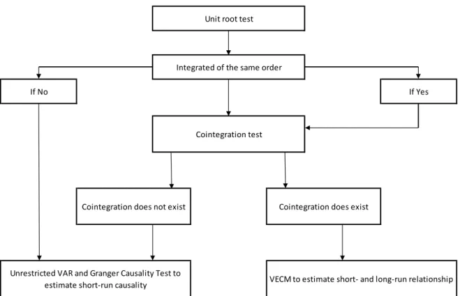
The current paper utilized panel unit root test in order to provide the stationarity properties of the variables considered, cointegration tests are performed to ascertain the presence of cointegration and then causality analyses in order to examine the interrelationship between the series. Panel data methods combine information from both time and cross-section dimensions, and as a result these methods increase the power of unit root and cointegration tests.

Figure 2. The empirical modelling framework.

Source: own figure, (Obadi and Korček, 2014)

The empirical modelling framework is outlined in Figure 2. The first step focuses on the stochastic stationarity properties of the variables by testing the presence of the unit roots and classifying the order of integration using panel unit root tests. This allows identifying stationary and non-stationary time series, which in turn allows for the model specification and avoidance of the spurious regression. In order to avoid statistical insignificance of coefficients and multicollinearity, the optimal lag length is then determined with application of Akaike information criterion (AIC) and Schwarz information criterion (SIC). Second, an unrestricted VAR is estimated involving potentially non-stationary variables. Then, the cointegration test is applied by implementing Johansen test to ascertain the presence of cointegration and the long-run cointegration parameters are estimated. If the cointegration exists among variables, causal

Cointegration does not exist Cointegration does exist

VECM to estimate short- and long-run relationship Unrestricted VAR and Granger Causality Test to

estimate short-run causality

Unit root test

Integrated of the same order

Cointegration test

If Yes If No

(22)

relationships are analysed based on the panel VECM model. If cointegration does not exist, unrestricted VAR model is estimated and followed by the Granger Causality test.

3.2.1 Panel unit root analysis

The crucial step in empirical analysis is the determination of the order of integration of the variables, since the conventional OLS estimators with non-stationary variables leads to spurious results (Irz, Niemi & Liu, 2013). Many research studies rely on panel unit root tests for the purpose of increasing the statistical power of the estimators (Nazlioglu & Soytas, 2012; Olayungbo & Hassan, 2016). The panel unit root tests entail estimating the following panel model:

∆𝑦𝑖𝑡 = 𝜇𝑖 + 𝜌𝑖𝑦𝑖𝑡−1+ ∑𝑗=1𝑘 𝛼𝑖𝑗∆𝑦𝑖𝑡−𝑗+ 𝛿𝑖𝑡 + 𝜃𝑡+ 𝜀𝑖𝑡 (4)

where Δ is the first difference operator, 𝑘 is the lag length, 𝜇_𝑖 and 𝜃_𝑡 are unit-specific fixed and time effects, respectively.

There are two types of panel unit root processes. Fist type is called a common unit root process

when the persistence parameters are common across cross-sections. The null hypothesis is 𝜌𝑖=0

for all i is tested against the alternative hypothesis of 𝜌_𝑖<0 for all i. The null hypothesis implies that all series are non-stationary and have a unit root while the alternative hypothesis implies a panel stationary process. The strong assumption of homogenous 𝜌_𝑖 is difficult to satisfy, as cross-sections may have different speed of adjustment towards the long-run equilibrium (Nazlioglu & Soytas, 2012).

Second type is characterized by the persistence of parameters moving freely across cross-sections and is called an individual unit root process. The null hypothesis of 𝜌𝑖=0 for all i is

tested against the alternative hypothesis of 𝜌_𝑖<0 for at least one i. The null hypothesis accordingly implies that all series are non-stationary and have a unit root while the alternative hypothesis implies that some of the series are stationary. Thus, the rejection of null hypothesis suggests stationarity of some of the series in the panel data (Serra & Zilberman, 2013).

In this respect, three unit root tests were employed in the current work: the unit root test developed by Levin, Lin and James Chu (2002) that assumes common unit root process, and two unit root tests, Augmented Dickey and Fuller (1979) (ADF) and Phillips and Perron (1988) (PP) tests, that assume individual unit root process. The tests are conducted with two alternatives for each type of test: consideration of constant trend and consideration of both

(23)

constant coefficient and trend. The lag length for each test is automatically selected by SIC criterion.

3.2.2 Panel cointegration analysis

Prior to estimating long-run model, the cointegration relationship between the variables of interest need to be determined. According to Engle and Granger (1987), two series integrated of the same order 𝑑, 𝐼(𝑑), are co-integrated, if their linear combination generates a stationary series. The series that are non-stationary and co-integrated may move away in the short run but must be linked together in the long run. The cointegration analysis implies testing the existence of a long run relationship between co-integrated variables that never move far apart and are attracted to their long run relationship (Nwoko, Aye & Asogwa, 2016).

There is a variety of methods for testing the cointegration between series and for the purpose of this study the Johansen-Fisher cointegration test was implemented in order to capture the long-run relationship between variables of interest. The Johansen-Fisher cointegration framework allows determining the number of co-integrating vectors among series but its weakness is that it is based on asymptotic properties and requires the variables to be integrated of the same order. The pre-testing is done by the unit root test discussed above and if the series are integrated of the same order, the estimation of long run equilibrium relationship follows.

The Johansen-Fisher cointegration test is based on unrestricted VAR. Consider a general 𝑝 –

dimensional, 𝑘th_{order panel unrestricted VAR:}

𝑦_𝑖𝑡 = ∑𝑘𝑖 Π_𝑖𝑘𝑦_{𝑖,𝑡−𝑘}+ 𝜀_𝑖𝑡

𝑘=1 (5)

where i=1, 2,…,N cross-section units and t=1, 2,…, T time periods, and 𝜀_𝑖𝑡 are errors that are

assumed to be independent and Gaussian with zero mean and covariance matrix Ω,

𝜀𝑖𝑡~𝑁𝑃(0, Ω𝑖).

The error correction form of VAR:

∆𝑦_𝑖𝑡 = Π_𝑖𝑦_{𝑖,𝑡−1}+ ∑𝑘𝑖−1Γ_𝑖Δ𝑦_{𝑖,𝑡−𝑘}+ 𝜀_𝑖𝑡

𝑗=1 (6)

where Δ𝑦_𝑖𝑡 is a 𝑝 x 1 vector of endogenous variables, 𝑝 is a number of variables, Γ₁through

Γ𝑘−1(𝑝 x 𝑝) and Π𝑖 (𝑝 x 𝑝) are matrix of parameters to estimate for 𝑘 order of lags and 𝑟 =

(24)

According to Engle and Granger (1987), if all the variables in 𝑦𝑡 are integrated of order 𝑑, and

there exists a co-integrating vector 𝛽𝑖 ≠ 0 such that 𝛽′𝑖𝑦𝑖𝑡 is integrated of order 𝑑 − 𝑟, then the

process in 𝑦_𝑖𝑡 is co-integrated of order CI (𝑑, 𝑟). If the 𝑟𝑎𝑛𝑘(Π_𝑖) = 0, the model represented by equation (6) is reduced to a differenced vector time-series model and no co-integration exists among variables in 𝑦𝑖𝑡. If 0 < 𝑟𝑎𝑛𝑘(Π𝑖) < p, there exists two matrices α𝑖 (𝑝 x 𝑟) and

β𝑖 (𝑝 x 𝑟) each with a rank 𝑟 such that Π𝑖 = 𝛼𝑖𝛽′𝑖. 𝛽′𝑖 consists of 𝑟 co-integrating vectors and

represents the long run relationship between the variables in 𝑦_𝑖𝑡, while α_𝑖 represents the speed of adjustment to the long-run equilibrium. By assuming co-integration of order 𝑟 the equation (6) can be written as:

∆𝑦_𝑖𝑡 = 𝛼_𝑖𝛽′_𝑖𝑦_{𝑖,𝑡−1}+ ∑𝑘𝑖−1Γ_𝑖Δ𝑦_{𝑖,𝑡−𝑗}+ 𝜀_𝑖𝑡

𝑗=1 (7)

The model represented in equation (7) has the property that under suitable conditions on the parameters the process is non-stationary, ∆𝑦_𝑖𝑡 is stationary, and 𝛽′_𝑖𝑦_𝑖𝑡 is stationary.

In order to ascertain cointegration relationships, first optimal lag length (𝑘) is determined by the use of AIC and SIC and the cointegration rank (𝑟) is determined. For cointegration rank estimation, or the presence of cointegration vectors in non-stationary series, Johansen (1988) proposes two approaches – maximum eigenvalue statistics and likelihood ratio trace statistics. The advantage of the tests is that they do not specify the cointegration vectors, but examine how many stationary combinations can be made within the variables’ set.

𝜆𝑚𝑎𝑥(𝑟, 𝑟 + 1) = −𝑇𝑙𝑛(1 − 𝜆̂𝑟+1) (8)

𝜆𝑡𝑟𝑎𝑐𝑒(𝑟) = −𝑇 ∑𝑝𝑖=𝑟+1ln (1 − 𝜆̂𝑖) (9)

where 𝑇 is the sample size, 𝑝 is the number of variables, 𝑟 is the rank of cointegration, 𝜆̂_𝑖 is the ith_{eigenvalue of the co-integrating matrix.}

The maximum eigenvalue statistics shown as equation (8) performs separate tests on each eigenvalue. It tests a null hypothesis of existence of 𝑟 co-integrating vectors against the alternative of 𝑟 + 1 cointegration vectors. The trace test is a one sided test represented by the equation (9). It tests the null hypothesis of at most 𝑟 cointegration vector against the alternative hypothesis of full rank 𝑟 = 𝑝 cointegration vector.

Using Johansen cointegration test (1988), Maddala and Wu (1999) propose Fisher's suggestion (1926) to combine trace test and maximum eigenvalue statistics in order to test for cointegration in full panel by combining individual cross-section tests for cointegration.

(25)

If 𝜋𝑖 is the 𝑝-value from an individual cointegration test for cross-section i, then under the null

hypothesis for the whole panel,

−2 ∑𝑁𝑖=1𝑙𝑜𝑔𝑒(𝜋𝑖) (10)

is distributed as 𝜒_2𝑁2 _.

Johansen-Fisher panel cointegration test aggregates 𝑝-values of individual Johansen maximum likelihood cointegration test statistics. Unlike other panel cointegration tests (Pedroni and Kao) it is not residual based which is taken from Engle Granger two step test, rather it is system based cointegration for the whole panel set (Maddala & Wu, 1999).

3.2.3 Panel causality analysis

Since cointegration analysis does not identify the direction of causality, causal interactions among the variables need to be determined. In case of long-run relationship, panel VECM is implemented while panel VAR is applied in case of no cointegration. The models were then used to conduct Granger causality tests on the relationship between domestic food prices, international oil and food prices, U.S. dollar exchange rate and country inflation.

Panel unrestricted VAR model is estimated as follows: 𝑙𝑜𝑔_𝑓𝑝𝑙_𝑖𝑡 = 𝛼_𝑖 + ∑𝑘 𝛽_𝑖𝑗

𝑗=1 𝑙𝑜𝑔_𝑓𝑝𝑙𝑖𝑡−𝑗+ ∑𝑘𝑗=1𝛾𝑖𝑗𝑙𝑜𝑔_𝑜𝑖𝑙𝑖𝑡−𝑗+ ∑𝑘𝑗=1𝛿𝑖𝑗𝑙𝑜𝑔_𝑒𝑥𝑟𝑖𝑡−𝑗+

+ ∑𝑘𝑗=1𝜑𝑖𝑗𝑙𝑜𝑔_𝑓𝑝𝑔𝑖𝑡−𝑗+ 𝜀𝑖𝑡 (11)

where 𝑘 is the optimum number of lags, 𝛼𝑖 is country fixed effects.

The unrestricted VAR is specified in levels and the dependent variable 𝑙𝑜𝑔_𝑓𝑝𝑙𝑖𝑡 is a function

of its own lagged values and the lagged values of other variables in the model. However, as Engle and Granger (1987) showed, implications of causality based on a VAR model in first differences will be misleading in case the variables are co-integrated. In order to avoid such problem, is to estimate panel VECM by augmenting the VAR with one-lagged error correction term.

The panel VECM is obtained by differenciating VAR and can be presented as follows to get the direction of causality between the variables of interest:

Δ𝑙𝑜𝑔_𝑓𝑝𝑙_𝑖𝑡 = 𝛼_1𝑖+ ∑𝑘 𝛽_11𝑖𝑗

𝑗=1 Δ𝑙𝑜𝑔_𝑓𝑝𝑙𝑖𝑡−𝑗+ ∑𝑘𝑗=1𝛾12𝑖𝑗Δ𝑙𝑜𝑔_𝑜𝑖𝑙𝑖𝑡−𝑗+

(26)

where Δ is first difference, 𝑘 is the optimum number of lags, 𝛽, 𝛾, 𝛿, 𝜑 are short-run dynamic coefficients of the model’s adjustment long-run equilibrium, 𝐸𝐶𝑇𝑖𝑡−1 is an error correction term

and 𝜆_1𝑖 is a speed of adjustment parameter for each cross-section.

The VECM specification allows to investigate both short- and long-run causality. The causality can be identified by the significance of coefficients on the lagged variables in equation (12). The short-run Granger weak causality, for example, from oil prices to domestic food prices, is tested by imposing 𝛾_12𝑖𝑗 = 0 for all i. The long-run causality or weak exogeneity is determined by the statistical significance of the error correction term (ECT) which stands for the lagged values of residuals obtained from co-integrating regression of the dependent variable on the regressors and represents short-run adjustment to long-run equilibrium trends. The coefficient

of ECT 𝜆_1𝑖 represents how fast deviations from long-run equilibrium are adjusted following

changes in variable. If, for example, 𝜆1𝑖 is non-zero and significant, then 𝑙𝑜𝑔_𝑓𝑝𝑙𝑖𝑡 is Granger

caused in the long-run by the oil prices, exchange rates, global food prices, and inflation; in

other words, 𝑙𝑜𝑔_𝑓𝑝𝑙_𝑖𝑡 responds to a deviation from the long-run equilibrium in the previous

period.

The present work also checked whether the causation sources are jointly significant by implying the Granger causality test. The procedure involves testing the joint null hypothesis: 𝛾_12𝑖𝑗 = 0, 𝛿_12𝑖𝑗 = 0, 𝜑_12𝑖𝑗 = 0, 𝜇_12𝑖𝑗 = 0 and 𝜆_1𝑖 = 0 for all i in equation (12). This represents the strong Granger causality test. The joint test identifies variables that bear the burden of short-run adjustment to long-run equilibrium after a shock to the system.

(27)

4 Empirical data

In the present paper the Middle East region is defined as a transcontinental region bound by Egypt to the West, the Arab Peninsula to the South, Iran to the East, and Turkey to the North. There are 16 countries in the region, however, due to limited data access resulting from the current political instability in Iran, Iraq, Palestine, Syria, and Yemen, these countries were excluded from the empirical analysis. Thus, 11 countries were included in the empirical analysis consisting of Bahrain, Egypt, Israel, Jordan, Kuwait, Lebanon, Oman, Qatar, Saudi Arabia, Turkey, and UAE. The fact that this sample countries consists of both oil importing and oil exporting countries will help understand how the effect of oil prices on domestic food prices differs across resource-scarce and resource-abundant economies.

The data employed in the present work consists of monthly observations spanning from January 2010 to October 2018, providing 106 observations for each country considered. This period was grounded on the availability of monthly consumer price indexes (CPI) for food data as higher frequency data are unavailable.

Domestic food prices (fpl) are measured by the CPI for food commodity groups (FCPI). FCPI measures the price change between the current and reference periods of an average basket of food commodities purchased by households. Food price index, which is used as a proxy for the world food prices (fpg), is a measure of the monthly change in international prices of a basket of food commodities and consists of the cereal price index, vegetable oil price index, meat price index, sugar price index and dairy price index. The data for fpl and fpg were obtained from Food and Agriculture Organization of the United Nations database (FAOSTAT).

World oil price (oil) is the U.S. dollar price per barrel sourced from the Commodity Prices Database of International Financial Statistics (IFS). The impact of oil prices on agricultural commodity prices is expected to be positive. Oil prices are the important factor in the cost of food production. Hence, the increase in oil prices may cause higher market prices of agricultural commodities. Moreover, oil price growth may also increase demand for agricultural commodities that are also used for biofuels production which in turn results in increased food prices. The expected sign of the global food prices is positive as domestic price levels can be affected by world food prices and fast-growing domestic food demand due to population growth can cause inflationary pressures.

Exchange rates have long played an important role on the price formation and have had an impact on the export and import of products that are traded. The exchange rate (exr) represents

(28)

the real effective exchange rate of U.S. dollar and sourced from the Commodity Prices Database of IFS. It represents the measure of a weighted average of real exchange rates of the U.S. dollar against the weighted basket of currencies of its main trading partners. The expected sign of the exchange rate is grounded on its definition. The agricultural commodity prices are quoted in U.S. dollars in international markets and due to this exchange rate is described as a value of U.S. dollar in a way that a decrease reflects the depreciation of the currency against major international currencies. As the U.S. dollar weakness can result in growth of agricultural commodity prices through increased purchasing power and foreign demand, the impact of exchange rate on food prices is expected to be negative.

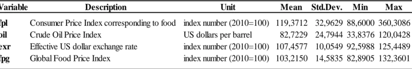
The whole data analysis was performed using natural logarithms and in order to avoid data inconsistency resulting from measuring prices in different units and to work with real values, the price indexes (2010=100) were used. The summary of the descriptive statistics for the variables across Middle East countries in the panel dataset provided in Table 1.

Table 1. Descriptive statistics of the time series variables.

Source: own calculations, 2019

Variable Description Unit Mean Std.Dev. Min Max

fpl Consumer Price Index corresponding to food index number (2010=100) 119,3712 32,9629 88,6000 360,3086

oil Crude Oil Price Index US dollars per barrel 82,7229 24,7944 33,8376 120,0428

exr Effective US dollar exchange rate index number (2010=100) 107,4577 10,0549 92,5988 125,4489

fpg Global Food Price Index index number (2010=100) 103,2150 14,5835 82,8905 132,3601 Observations: 1166

(29)

5 Results and discussion

The following section provides the results for two data types: the panel data results for the whole sample of the Middle East countries and the time-series data results for each individual country considered in the study. The discussion of the results is also presented in the section.

5.1 Full-sample results

This part of the analysis presents the results of panel unit root tests, Johansen cointegration test, followed by the estimates of VECM and Granger causality tests outcomes. Unit root tests showed that the variables are integrated of order one and Johansen cointegration test can be applied. The test revealed that variables are cointegrated in the long-run and VECM was applied.

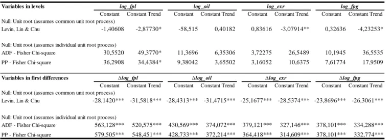
5.1.1 Panel unit root tests

The results of the panel unit root tests are reported in Table 2. For the levels of the variables, the results do not present a uniform conclusion that the null hypothesis can be rejected. However, the test–statistics for the first differences strongly reject the null hypothesis of the non-stationarity with the 1% significance level. Therefore, it can be concluded that the variables are integrated of order one, I(1), and this indicates a possibility of the long-run cointegration among the variables analyzed. Hence, the Johansen test for long-run cointegration follows in the next step of the data examination.

Table 2. Results for panel unit root tests.

Variables in levels

Constant Constant Trend Constant Constant Trend Constant Constant Trend Constant Constant Trend Null: Unit root (assumes common unit root process)

Levin, Lin & Chu -1,40608 -2,87730* -58,515 0,40182 0,83616 -3,07914** 0,32636 -4,23253*

Null: Unit root (assumes individual unit root process)

ADF - Fisher Chi-square 30,5520 49,3770* 11,3696 6,35306 3,72275 26,5489 10,1945 36,5535

PP - Fisher Chi-square 36,2908 34,4384* 9,38042 3,65502 3,16052 10,6375 7,61774 17,9509

Variables in first differences

Constant Constant Trend Constant Constant Trend Constant Constant Trend Constant Constant Trend Null: Unit root (assumes common unit root process)

Levin, Lin & Chu -28,1420*** -31,5818*** -28,4313*** -31,4715*** -25,1677*** -28,5374*** -23,8696*** -26,3061***

Null: Unit root (assumes individual unit root process)

ADF - Fisher Chi-square 563,128*** 520,575*** 430,569*** 374,072*** 379,121*** 327,146*** 378,101*** 334,288***

PP - Fisher Chi-square 579,505*** 548,451*** 428,733*** 372,214*** 364,418*** 314,609*** 378,101*** 332,774***

∆ is the first difference operator. The lag length for each variable was automatically selected by the Schwarz Information Criterion. ***p<0,01, **p<0,05, *p<0,1

log_fpl log_oil log_exr log_fpg

(30)

5.1.2 Johansen Fisher panel cointegration test

The result for panel cointegration test are presented in Table 3. The tests were performed for constant as well as constant and trend cases. The lag length of two was determined using AIC and SIC. All the test statistics reject the null hypothesis of no cointegration at 1% level for trace test and at 5% level for maximum eigenvalue test. The empirical findings provide strong evidence of cointegration among variables. This implies that domestic food prices in the sample of the Middle East countries converge to their long-run equilibrium by correcting the deviations from it in the short-run. Hence, this suggests the existence of long-run relationship among variables. The test results indicate that the model is fit for the estimation of panel VECM to better capture and predict causality results, of which at least one cointegration relationship exists among the variables.

Table 3. Johansen Fisher panel cointegration test results.

5.1.3 Panel VECM

The results of VECM are reported in Table 4 for the long-run parameters and in Table 5 for the short-run parameters. The long-run estimates reveal that the variables have long-run equilibrium relationship. The guideline is when the coefficient of cointegration equation is negative and significant there exists a long-run causality from the independent variables to the dependent variable. In other words, a negative and significant ECT indicates that short-run movements between independent and dependent variables are associated with a stable long-run relationship between variables (Obadi & Korček, 2014).

The coefficient of cointegration equation in Table 5 is -0,000102 with 5% significance value. This result indicates that domestic food prices are affected by the global oil prices, U.S. dollar strength, and global food prices in the long run. 1% increase in world oil prices, depreciation of the U.S. dollar and world food prices results in 6,35%, 6,21% and 2,67% increase in local

Hypothesized No. Of CE(s)

Constant Constant Trend Constant Constant Trend

None 37,28** 52,66*** 33,39** 34,62**

At most 1 18,18 29,07 15,10 18,26

At most 2 16,21 20,55 15,76 24,32

At most 3 17,01 8,441 17,01 8,441

Fisher Stat.* from trace test Fisher Stat.* from max-eigen test

Probabilities are computed using asymptotic Chi-square distribution. ***p<0,01, **p<0,05, *p<0,1

(31)

consumer price index for food in the sample of Middle East countries respectively. This is consistent with the literature, such as Rezitis (2015), Cabrera and Schulz (2016), and Zafeiriou et al. (2018).

Table 4. VECM long-run parameters.

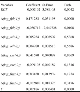
As for the short-run coefficients presented in Table 5, results show that domestic food prices do not respond to changes in oil prices, U.S. dollar effective exchange rate, and global food prices. There is no short-run causality from independent variables except to its own lagged one and lagged two price, which show statistical significance at 1% and at 5% level respectively. The lagged one coefficient implies the immediate possible price response of domestic food prices from independent variable, which is 0,17%; while lagged two is associated with response after one period or in this case after one month, which shows 0,08% increase.

Table 5. VECM short-run parameters.

Variables CointEq1 log_fpl(-1) 1,000000 log_oil(-1) 6,354506*** (0,956335) log_exr(-1) -6,207403*** (0,426306) log_fpg(-1) 2,674144*** (0,218742) C 4,415095 ***p<0,01, **p<0,05, *p<0,1 Notes: standard errors in ()

Variables Coefficient St.Error Prob.

ECT -0,000102 3,58E-05 0,0042 ∆(log_fpl(-1)) 0,171283 0,031198 0,0000 ∆(log_fpl(-2)) -0,080712 -2,549728 0,0108 ∆(log_oil(-1)) 0,005254 0,008507 0,5368 ∆(log_oil(-2)) 0,004980 0,008513 0,5586 ∆(log_exr(-1)) 0,041670 0,040097 0,8369 ∆(log_exr(-2)) -0,009105 0,040189 0,1316 ∆(log_fpg(-1)) 0,003180 0,017939 0,1234 ∆(log_fpg(-2)) -0,032810 0,018325 0,3176 C 0,002186 0,000481 0,0000

(32)

5.1.4 Granger causality Wald test

Granger causality tests were conducted by testing the joint hypothesis that the coefficient of ECT and coefficients of differenced lagged variables in estimated VECM are zero against the alternative that they are not. The null hypothesis that the independent variable does not Granger cause the dependent variable is tested with the use of F-statistic. The results of Granger causality tests are reported in Table 6. The findings show that only the change in global food prices Granger causes the change in domestic food prices with the 10% significance level. However, on the aggregate level all independent variables Granger cause changes in domestic food prices with 5% level of significance.

Table 6. Granger causality test results.

Generally, the Granger causality test shows the significant results only on the aggregate level and the VECM model provides evidence of the long-run relationship of the price variables taken into consideration. The short-run dynamics are relatively less helpful and require further examination as most of the estimates are insignificant. Moreover, in order to determine whether oil impact differs across resource rich and resource poor countries in the sample of the Middle East region the investigation proceeds with the time series analysis of individual country cases to obtain deeper understanding of price series interdependencies.

5.2 Country-level results

The current section concentrates on the causality analysis based on the time series data for each individual country in the sample. The same step-by-step procedure has been followed as outlined in Section 3.2 and illustrated in Figure 2 but only for the time series dataset.

For each time series of individual countries the ADF and PP tests were implied to the price series for 11 countries considered. The results are shown in Table 7 and indicate that all variables are I(1), integrated of order one, which implies that in levels the variables have unit roots and thus non-stationary, given that the null hypothesis cannot be rejected at any conventional significance level. However, in first difference, the null hypothesis of unit root is rejected by both ADF and PP unit root tests whether the deterministic trend is included or not.

Excluded Chi-sq df Prob.

∆log_oil 11,8582 2 0,2214

∆log_exr 10,8009 2 0,2896

∆log_fpg 15,4437 2 0,0794

(33)

Table 7. Unit root tests results.

Johansen cointegration test

The results of Johansen cointegration tests are reported in Table 8. The findings do not show a uniform conclusion for the 11 countries. There exists a long-run relationship in Bahrain, Egypt, and Kuwait as p-values for these countries show the significance at 5% level. It implies that the global crude oil prices and domestic food prices of these countries move together over time providing that in case of the deviation from the mean level or equilibrium level, the variables will be easily brought back to equilibrium. While the variables are nonstationary, their linear combination is stationary and overall oil and food prices have the long-run significant relationship in Bahrain, Egypt and Kuwait.

The statistics provide strong evidence for the cointegration, which suggests that local prices in Bahrain, Egypt and Kuwait converge to their long-run equilibrium by correcting any deviation from this equilibrium in the short-run. For other countries in the sample Johansen test did not reveal cointegration relationship between the variables. Thus, for Bahrain, Egypt, and Kuwait the VECM is estimated, while for Israel, Jordan, Lebanon, Oman, Qatar, Saudi Arabia, Turkey and UAE the unrestricted VAR is applied.

Variable Country Constant C-Trend Constant C-Trend Constant C-Trend Constant C-Trend log_fpl Bahrain -1,3655 -1,6893 -1,2444 -1,4287** -7,3243*** -7,2902*** -7,3051*** -7,2703*** log_fpl Egypt 0,7842 -1,3150 1,1383 -0,8173 -6,3751*** -6,4659*** -5,9281*** -5,8060*** log_fpl Israel -2,6454 -2,7313 -2,6065 -2,6670 -10,2570*** -10,2562*** -10,3003** -10,3233** log_fpl Jordan -2,3182 -1,7827 -2,4221 -1,8085 -9,3608*** -9,5266*** -9,8736*** -10,4065** log_fpl Kuwait -3,3512* -1,4845 -3,5265* -1,4565 -9,2787*** -10,0529*** -9,3127*** -10,0710** log_fpl Lebanon -1,6354 -2,5075 -1,8434 -2,2878 -7,8095*** -7,8023*** -7,6382*** -7,7129*** log_fpl Oman -2,7907 -2,8002 -2,9758** -1,9380 -7,9068*** -7,9966*** -7,7347** -8,4054*** log_fpl Qatar -2,2741 -2,6708 -2,2745 -2,6708 -9,5005*** -9,4974** -9,4771*** -9,4679***

log_fpl Saudi Arabia -1,0885 -2,3799 -1,1931 -2,4533 -9,8724*** -9,9359*** -9,8723*** -9,9359***

log_fpl Turkey 0,9801 -3,6038* 1,8647 -1,9139 -6,6941*** -6,8725*** -8,4921*** -8,9990***

log_fpl UAE -1,8714 -2,4663 -2,3331 -2,3866 -9,0196*** -9,1024*** -9,1494*** -10,3120**

log_oil World -1,3655 -1,6894 -1,2445 -1,4287 -7,3243*** -7,2902*** -7,3051** -7,2703***

log_exr United States -0,6879 -2,5606 0,5945 -1,9586 -6,7856*** -6,7876*** -6,6313*** -6,6525***

log_fpg World -1,2963 -2,8308 -1,1162 -2,2772 -6,7749*** -6,8644*** -6,7749*** -6,8478***

Notes: the critical values are -2,89 and -3,45 at 5% significance for a constant equation and a constant-trend equation, respectively. Notes: ***p<0,01, **p<0,05, *p<0,1

ADF test statistics PP test statistics Test on level variables

ADF test statistics PP test statistics Test on first-differenced variables