THESIS
ANALYSIS AND CHARACTERIZATION OF WIRELESS SMART POWER METER
Submitted by Sachin Soman
Department of Electrical and Computer Engineering
In partial fulfillment of the requirements For the Degree of Master of Science
Colorado State University Fort Collins, Colorado
Summer 2014
Master’s Committee:
Advisor: Peter Young Daniel Zimmerle Sudeep Pasricha
ii ABSTRACT
ANALYSIS AND CHARACTERIZATION OF WIRELESS SMART POWER METER
Recent increases in the demand for and price of electricity has stimulated interest in monitoring energy usage and improving efficiency. This research work supports development of a low-cost wireless smart power meter capable of measuring VRMS, IRMS, real power, and reactive power. The proposed smart power meter features include matching by-device rate of consumption and usage patterns to assist users in monitoring the connected devices. The meter also includes condition monitoring to detect harmonics of interest in the connected circuits which can give vital clues about the defects in machines connected to the circuits. This research work focuses on estimating communicational and computational requirements of the smart power meter and optimization of the system based on the estimated communication and computational requirements.
The wireless communication capabilities investigated here are limited to existing wireless technologies in the environment where the power meters will be deployed. Field tests are performed to measure the performance of selected wireless standard in the deployment environment. The test results are used to understand the distance over which the smart power meters can communicate and where it is necessary to utilize repeaters or range extenders to reduce the data loss.
Computational requirements included analysis of smart meter front-end sampling of analog data from both current and voltage sensors. Digitized samples stored in a buffer which is further processed by a microcontroller for all the desired results from the power meter. The various stages for processing the data require computational bandwidth and memory dependent on the
iii
size of the data stream and calculations involved in the particular stage. A Simulink-based system model of the power meter was developed to report a statistic of computational bandwidth demanded by each stage of data processing.
The developed smart meter works in an environment with other wireless devices which include Wi-Fi and Bluetooth. The data loss caused when the smart power meter transmits the data depends on the architecture of the wireless network and also pre-existing wireless technology working in the same environment and while operating in the same frequency band. The best approach in developing a wireless network should reduce the hardware cost of the network and to reduce the data loss in the wireless network. A wireless sensor network is simulated in OMNET++ platform to measure the performance of wireless standard used in smart power meters. Scenarios involving the number of routers in the network and varying throughput between devices are considered to measure the performance of wireless power meters.
Supplementary documents provided with the electronic version of this thesis contain program codes which were developed in Simulink and OMNET++.
iv
ACKNOWLEDGEMENTS
I would like to take this opportunity to thank all the people who helped me to complete this project. First and foremost, I would like to express my sincere gratitude to my advisor-Dr. Peter Young for his continuous support in my research. Next, I would like to thank Professor Daniel Zimmerle for his advice and encouragement throughout the project. His expertise, understanding and patience added considerably to my experience in graduate school. I would also like to acknowledge Dr. Sudeep Pasricha for his role as a member of my defense examination committee. Additionally, I would like to thank Jerry Duggan for his suggestions on various phases of the project and I wish to thank all the staff in Engines and Energy Conversion Laboratory for their kind help during various stages of my graduate program.
I would also like to acknowledge the financial support for this work provided by Colorado State University Clean Energy Supercluster grant, “Development of Low-Cost Conditioning Monitoring using Wireless Microcontroller Electricity Measurements,” and support provided by InGreenium, LLC under Department of Energy grant DE-SC0009210 from program
v TABLE OF CONTENTS Abstract…...……….…………....ii Acknowledgements………..………...iv Table of Contents………...v List of Tables………..….x List of Figures………....……….xi Introduction ... 1 1 Overview ... 1
1.1 Need for Power Metering ... 1
1.2 Types of Power Meters ... 2
1.2.1 Utility Power Meters ... 2
1.2.2 Analog Meters ... 2
1.2.3 Power Quality Meters... 3
1.2.4 Low Cost Power Meter ... 3
1.3 The Proposed Smart Meter ... 3
1.3.1 Subpanel Implementation ... 4
1.4 Functions of Proposed Smart Power Meter ... 6
1.4.1 Root Mean Square (RMS) Measurement ... 6
1.4.2 Real Power Measurement... 8
1.4.3 Reactive Power Measurement ... 10
vi
1.4.5 Pattern Matching ... 13
1.5 Computational and Data Communication Requirements of the Proposed Smart Power Meter. ... 14
1.5.1 Per-Cycle Measurements... 14
1.5.2 Condition Monitoring ... 15
1.5.3 Pattern Matching ... 15
1.6 Communication Features of Smart Meter ... 16
1.7 Hardware Platform of Smart Power Meter ... 18
1.8 Smart Power Meter – Architecture ... 19
1.8.1 Stage 1 ... 19
1.8.2 Stage 2 ... 20
1.8.3 Stage 3 ... 20
1.9 Component Decisions for Smart Power Meter ... 20
1.10 Thesis Overview ... 20
1.11 References ... 22
Zigbee Radio Range Testing ... 25
2 Overview ... 25
2.1 Introduction ... 25
2.1.1 Zigbee Protocol Stack ... 26
2.1.2 Zigbee Frequency of Operation... 27
vii
2.1.4 Coexistence with Wi-Fi ... 29
2.2 Test Setup – Zigbee Performance Measurement ... 31
2.2.1 Experiment 1 ... 33
2.2.2 Experiment 2 ... 34
2.3 Test Results ... 36
2.4 Conclusion ... 37
2.5 References ... 41
Digital Filter Overhead Estimation ... 43
3 Overview ... 43
3.1 Introduction ... 43
3.1.1 Factors to Consider for Filter Selection ... 44
3.1.2 Implementation in Smart Power Meter ... 45
3.2 Estimation of Computation Overhead ... 48
3.3 Test Cases ... 49 3.3.1 Test Case-1 ... 50 3.3.2 Test Case-2 ... 50 3.4 Results ... 51 3.5 Conclusion ... 52 3.6 References ... 53
System Modeling – Smart Power Meter ... 54
viii
4.1 Introduction ... 54
4.2 The Simulink Model ... 56
4.2.1 ADC Interrupt Generator ... 57
4.2.2 Queue System ... 57
4.2.3 Microcontroller... 59
4.2.4 Functioning of Developed Model ... 64
4.2.5 Test Parameters ... 65
4.2.6 Measurement of Test Parameters ... 66
4.2.7 Simulation Parameters... 66
4.3 Results ... 67
4.4 Conclusion ... 69
4.5 References ... 70
Wireless Sensor Network Simulation - Zigbee Network ... 71
5 Overview ... 71
5.1 Introduction ... 71
5.1.1 Zigbee Device Types ... 72
5.1.2 Discrete Event Simulation ... 72
5.1.3 Zigbee based Energy Metering ... 75
5.1.4 Zigbee Data Communication ... 76
ix
5.2 The proposed Wireless Sensor Network ... 78
5.2.1 Assumptions ... 79
5.2.2 The Simulation ... 80
5.2.3 Results ... 89
5.3 Future Work ... 92
x LIST OF TABLES
Table 1.1: Computations for RMS and Power Calculation ... 14
Table 1.2: Data rates of popular communication schemes ... 16
Table 2.1: Zigbee Comparison with Wireless Standards [5] ... 27
Table 2.2: Zigbee Channels [6] ... 30
Table 3.1: Filter Computations [1] ... 49
Table 3.2: Test Case 1 Implementation of Downsampler System ... 50
Table 3.3: Test Case 2 Implementation of Downsampler System ... 50
Table 4.1: Primary Configuration Parameters ... 66
Table 4.2: Secondary Configuration Parameters ... 67
Table 4.3: Test Results ... 67
Table 5.1: Probabilistic Distribution for Power Packet Generation ... 81
Table 5.2: Network (Device and Clients under device) ... 88
Table 5.3: Throughput between devices ... 88
Table 5.4: Results (Scenario 1) ... 89
Table 5.5: Results (Scenario 2) ... 89
xi LIST OF FIGURES
Figure 1.1: Configuration – I ... 4
Figure 1.2: Configuration II ... 5
Figure 1.3: Algorithm for RMS Calculation ... 7
Figure 1.4: Algorithm for Real Power Calculation ... 9
Figure 1.5: Algorithm for Reactive Power Calculation ... 11
Figure 1.6: Smart Power Meter – Software Architecture ... 19
Figure 2.1: IEEE 802.15.4 Protocol Stack [1] ... 26
Figure 2.2: Zigbee Protocol Comparison (Range Vs. Data Rate) [5] ... 28
Figure 2.3: Zigbee Performance Test Setup ... 32
Figure 2.4: 2.4 GHz Spectrum (WIFI Environment) ... 34
Figure 2.5: 2.4 GHz Spectrum (Experiment 2) ... 35
Figure 2.6: Zigbee Radio Performance with WIFI Interference (Packet Loss Vs. Distance (meters)) ... 36
Figure 2.7: Zigbee Radio Performance in Environment Without WIFI (Packet Loss Vs. Distance (meters)) ... 37
Figure 2.8: Example of PCB board with Zigbee radio mounting pins ... 39
Figure 2.9: Proposed Performance Improvement Scheme for Zigbee Module ... 40
Figure 3.1: Front End System of Data Flow ... 45
Figure 3.2: A Typical Downsampler ... 46
xii
Figure 3.4: Results of Downsampler Implementation – Test Case 1 ... 51
Figure 3.5: Results of Downsampler Implementation – Test Case 2 ... 51
Figure 4.1: Simulink Model ... 56
Figure 4.2: Event Queue in Simulink Model ... 58
Figure 4.3: Microcontroller in Simulink Model ... 60
Figure 4.4: Condition Monitoring/Patter Matching Handler ... 62
Figure 4.5: Event Flow in Simulink Model ... 64
Figure 4.6: Timing Distribution (Stages in Algorithm) ... 68
Figure 5.1: Event Queue (OMNET++) ... 73
Figure 5.2: Proposed Zigbee Network ... 78
Figure 5.3: The Zigbee Network (OMNET++ Environment) ... 80
Figure 5.4: State Diagram – Client ... 82
Figure 5.5: State Diagram – Channel ... 84
Figure 5.6: State Diagram - Router ... 85
Figure 5.7: The Zigbee Network (Scenario 1) ... 87
Figure 5.8: The Zigbee Network (Scenario 2) ... 87
1 Chapter 1 Introduction 1 Overview
This chapter introduces the importance of measuring power and surveys electric power meters available in the current market. This is followed by proposed implementation and features of the smart power meter. The computational and communication bandwidth required for the proposed smart meter are also estimated. The final section of this chapter outlines the remaining sections of this thesis.
1.1 Need for Power Metering
Electricity pricing can motivate organizations to reduce energy use. The key to reducing electricity bills is to provide customers with a better understanding of when and where electricity is consumed, a key benefit of smart power meters. The energy usage data from these devices can also be used to improve the facility and limit the loss of energy [1.1]. The installation of power meters helps residential customers to have an understanding of energy usage in home. Wireless displays in these power meters can display real time costs of energy usage and can help customers to budget the energy usage [1.5].
Organizations can choose among many ways to reduce energy costs. Using power meters to detect power transients occurring in an event of start or stop of a device is relevant in this study of smart power meters. Start and stop information is used to calculate the operation time and duration. This data can be used in for scheduling of heating, ventilation and air conditioning (HVAC) to optimize energy usage [1.3] of the organization.
Beyond energy cost savings, power monitoring can enhance operational effectiveness by enhancing equipment maintenance capabilities. The energy consumption history of generators
2
and motors can be used to predict or detect the faults in the machine. The faults introduce identifiable harmonic components in the stator current of machines [1.6]. When detected, these harmonic components can give vital clues about the type of fault in the machine which includes bearing, eccentricity and gearbox faults. This information can help diagnose failures to speed repairs or to proactively manage maintenance to avoid downtime.
1.2 Types of Power Meters
Power meters are available in various configurations ranging from simple energy meters to complex meters which support power quality analysis and remote power management functions. Power meters can be broadly classified based on their functionality as described in this section.
1.2.1 Utility Power Meters
Utility power meters are installed in residential, commercial or industrial electric systems by utility companies for the primary purpose of billing. Recent innovations include built-in communication schemes to integrate with a central monitoring system. The communication schemes of these power meters include Power Line Communications (PLC), MODBUS over IP adapters etc. [1.7]. A utility power meter also detects sags, swells, transients and flickers in the electric line. The advanced version of utility power meters by Quadlogic [1.7] measures advanced metrics which includes power factor per phase, Total Harmonic Distortion (THD), voltage transients and current transients. Smart meters used by utilities cost between $250 and $500 [1.9] which does not include labor costs.
1.2.2 Analog Meters
The Analog power meter works on the principle of electro-mechanic induction. This meter operates by making an electrically conductive metal disc rotate at a speed proportional to
3
the power flowing through the meter. Typically, these traditional utility meters are not equipped with communications technology and the utility company sends an employee to record the power flow at regular intervals. Analog meters are inaccurate because of power consumed by rotating coils and friction between the rotating coils.
1.2.3 Power Quality Meters
Power quality meters are the advanced type of power meters compared to the two classifications listed above. Power quality meters measures single phase or 3 phase power in kWh and have advanced features which includes measurement of harmonic distortions (harmonic analysis through as high as the 63rd harmonic) and power quality metrics and can record user defined events [1.10]. These meters operate in wide voltage range. Power quality meters also have protection mechanisms to cope against voltage, current and frequency imbalances [1.10]. As an example, an Eaton Xpert Meter [1.8] has features which include a connection to a web server to analyze waveforms, trends and harmonics. Eaton Xpert meters are installed in large industries and are list- priced near $10,000.
1.2.4 Low Cost Power Meter
Low-cost power meters are priced in the range $50-$100 [1.20]. These basic power meters take in three phase 120/240V 3-wire 100 Amp line and displays real power in an integrated LCD display.
1.3 The Proposed Smart Meter
The proposed smart power meter measures VRMS. IRMS, real power and reactive power. The power measurements are used in advance features of the smart power meter which includes detecting harmonic components and tracking load time. These features are similar to those available in utility and power quality meters discussed in Section 1.2.1 and Section 1.2.3. The
4
proposed smart meter is similar to the Powerhouse Dynamics SiteSage and competing products, priced under $1000 [1.21] [1.22].
1.3.1 Subpanel Implementation
The proposed power meter is implemented in two configurations. 1.3.1.1 Configuration I
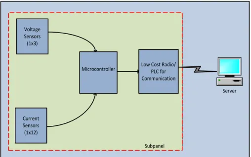
The proposed power meter is deployed in a subpanel and monitors 12 circuits in the subpanel. Current Sensors (1x12) Voltage Sensors (1x3)
Microcontroller Low Cost Radio/PLC for Communication
Server
Subpanel
Figure 1.1: Configuration – I
Figure 1.1 shows the implementation of a power meter in a subpanel which has 12 circuits attached to it. The three phase voltage is common for all circuits and there are 12 lines to monitor the current. The calculation of power in these 12 circuits requires three phase voltage value and 12 values of current. Thus, a single power meter can perform all the promised functions in 12 lines. The current sensors are clip-on current transformers attached to the wire exiting the subpanel to each circuit from the subpanel. A power supply is also tapped from voltage sensors to power all the components of the smart power meter. In this implementation,
5
each subpanel system requires a microcontroller and radio to measure and report power consumption of subpanel circuits.
1.3.1.2 Configuration II
The Figure 1.2 shows the implementation of the proposed smart power meter in configuration II.
Low Cost Radio/ PLC for Communication Server Voltage Sensors Board Current Sensor Board High S peed USB High S peed U SB Subpanel Central Microcontroller Figure 1.2: Configuration II
In this configuration voltage and current sensors are integrated into a board with a microcontroller. These boards are connected to a central microcontroller (common for a subpanel) via high speed USB connection. The central microcontroller is responsible for executing algorithms required to satisfy the promised functions of the smart power meter which are discussed in Section 1.4.2. This central microcontroller is high-power microcontroller with a dedicated USB memory to store data points from voltage and current sensor boards. The central microcontroller monitors up to 42 circuits.
6 1.4 Functions of Proposed Smart Power Meter The smart meter has the following functions: 1.4.1 Root Mean Square (RMS) Measurement
The RMS measures ‘heating’ potential of a signal. The Smart power meter measures RMS of current and voltage signals. RMS measurement of continuous signal is as follows [1.12]:
𝑉𝑅𝑀𝑆 = √1 𝑇𝑚∫ 𝑣2 𝑇𝑚 0 (𝑡)𝑑𝑡 1 𝐼𝑅𝑀𝑆= √ 1 𝑇𝑚∫ 𝑖2 𝑇𝑚 0 (𝑡)𝑑𝑡 2
v(t) and i(t) are the instantaneous values of voltage and current. Tm is the length of
a single period of the measured analog signal.
RMS measurement of discrete signal is as follows [1.8]:
𝑉𝑅𝑀𝑆= √1 𝑁∑ 𝑣2 𝑁 (𝑛) 3 𝐼𝑅𝑀𝑆 = √1 𝑁∑ 𝑖2 𝑁 (𝑛) 4 𝑣(𝑛) and 𝑖(𝑛) are the corresponding discrete values of voltage and current. N is the number of samples in a single period of the discrete signal. The sampling frequency of current and voltage signals should be an integral multiple of the fundamental component (60 Hz) to avoid any chance of aliasing.
7
Figure 1.3 describes the algorithm for RMS calculation implemented in the microcontroller.
Start
Receive Digitized Values of Voltage and Current (v(n) and i(n))
Square digitized value v(n) = v2(n)
i(n) = i2(n)
n = n+1
Add and Accumulate RMS = v2(n-1)+v2(n) Is N = n? No Result = RMS*(1/N) Yes Store Result in Buffer
N is number of samples in 1 cycle n = 1
Stop
Figure 1.3: Algorithm for RMS Calculation
In the first step, instantaneous values of voltage and current are received from Analog to Digital Converters (ADC). These digital values are multiplied with itself (Squared). The resulting values are accumulated. The accumulated value is multiplied by a stored number (1/N) to produce the final result from microcontroller. This value is stored in buffer and is sent to the server where square root operation is performed. Square root operation is performed in the server
8
to reduce the computational steps performed for RMS calculation in the microcontroller. In this algorithm, calculation of a single RMS value requires N additions and 1 multiplication.
1.4.2 Real Power Measurement
The Real power or true power denoted by P, measured in watts and is calculated as follows [1.12]:
𝑝 = 𝑣 × 𝑖 5
Real power of a continuous time signal is measured as follows [1.12]:
𝑝 = 1 𝑇𝑚∫ 𝑣
𝑇𝑚
0 (𝑡) × 𝑖(𝑡)𝑑𝑡 6
𝑣(𝑡) and 𝑖(𝑡) are instantaneous values of current and voltage. Real power is measured in discrete time signal as follows [1.12]:
𝑝 = 1
𝑁∑ 𝑣(𝑛) × 𝑖(𝑛)
𝑁 7
𝑣(𝑛) and 𝑖(𝑛) are instantaneous discrete values of current and voltage. N is the number of samples in a single cycle of fundamental component (60 Hz). The sampling frequency of current and voltage signals should be integral multiples of the fundamental component to avoid any chance of aliasing.
Figure 1.4 is the algorithm for real power calculation. In the first step, instantaneous values of V and I are received and are multiplied to calculate instantaneous power. Instantaneous power values are accumulated for a single cycle of the fundamental component. The resulting value is multiplied by 1/N where N is number of samples in a single cycle of the fundamental component.
9 P(a) = V(a)*I(a) n = n+1 Store Result in Buffer Stop Analog To Digital Converter Start
Add and Accumulate P(a) = P(a-1)+P(a)
Is N = n?
N = number of samples in 1 cycle n = 1
Receive Analog signal – V and I
No
Real Power = P*(1/N) n =1
Yes
10 1.4.3 Reactive Power Measurement
The magnitude of the reactive power (S) is calculated as follows [1.12]:
𝑆 = 𝑉𝐼𝑠𝑖𝑛𝜃 8
The Reactive power or apparent power measured in volt-amperes (VA) is calculated by implementing a time delay between voltage and current signals. This is based on the assumption that implementing a phase shift of 𝜋4 in either 𝑣 or 𝑖 and multiplying it produces the same result as in equation 8. This method is accurate only if signals 𝑣 and 𝑖 contain only the fundamental component (60 Hz). The phase shift is implemented by shifting the voltage signal by a quarter cycle. 𝑆 = 1 𝑇∫ 𝑣(𝑡) × 𝑖(𝑡 + 𝑇 4 𝑇 0 )𝑑𝑡 9
The reactive power algorithm is implemented by delaying voltage signals by a pre-defined number of samples equal to quarter cycle of the fundamental component (60 Hz) of the current signal. If the data is sampled at 3600 Hz and the fundamental component (60 Hz), then one cycle contains 60 samples. Hence, a quarter cycle of the fundamental component contains 15 samples. In the implementation, a data array is used to store 15 samples of voltage signals. The current samples are sequentially multiplied by stored voltage samples, buffered, and then sent to the server.
11
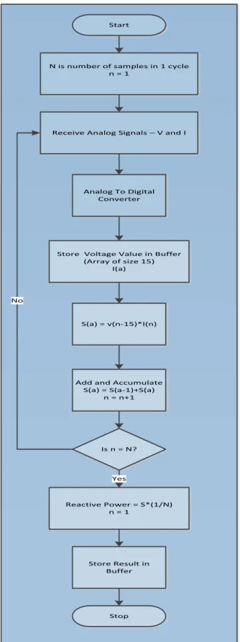
Start
N is number of samples in 1 cycle n = 1
Receive Analog Signals – V and I
Store Voltage Value in Buffer (Array of size 15) I(a) S(a) = v(n-15)*I(n) Store Result in Buffer Stop Add and Accumulate
S(a) = S(a-1)+S(a) n = n+1 Is n = N? Reactive Power = S*(1/N) n = 1 Yes No Analog To Digital Converter
12
Figure 1.5 describes the algorithm for reactive power calculation. In the first step, instantaneous values of current and voltage are received. The voltage value is multiplied by a delayed current value. The current value is delayed by quarter cycle of the fundamental component. The power values are accumulated for a single cycle of the fundamental component. The resulting value is multiplied by 1/N where N is the number of samples in a single cycle of the fundamental component.
1.4.4 Condition Monitoring/Frequency Analysis
The proposed power meter uses Discrete Fourier Transform (DFT) [1.10] to check the presence of harmonics. DFT is the mathematical transformation which gives both the amplitude and phase information of the desired frequency. A DFT is computed by using following equation: 𝑋ℎ= ∑ 𝑥(𝑛)𝑒 −𝑗2𝜋ℎ𝑛 𝑁 𝑁−1 𝑛= 0 10 where:
N is the block size that controls the resolved frequency in DFT x(n) is the signal at point n.
Xh is the Fourier vector of hth harmonic of the input signal.
𝑋ℎ = 𝑋ℎ𝑟+ 𝑗𝑋ℎ𝑖 11
where Xhr and Xhi are real and imaginary parts of Xh. Amplitude of harmonic component |𝑋ℎ| is given by,
|𝑋ℎ| = √𝑋ℎ𝑟2+ 𝑋 ℎ𝑖 2
12
13 𝜙𝑛 = 𝑎𝑟𝑐𝑡𝑎𝑛 𝑋ℎ𝑖 𝑋ℎ𝑟 13 1.4.5 Pattern Matching
Electric machines are often expensive to repair after a failure [1.19]. If a machine failure can be detected early, the cost of downtime, service and repair can be reduced. One of the features of the proposed smart meter is to detect the event of start/stop of the load. Changes in load run times or power drawn during operation can be signs of machine failure and detecting these events can help to schedule proactive maintenance. This project utilizes algorithms for detecting start and stop events described in [1.19].
The key computation for pattern matching is the calculation of several high-order statistical measures which includes the bimodality coefficient.
𝐵𝑖𝑚𝑜𝑎𝑑𝑖𝑙𝑖𝑡𝑦 𝑐𝑜𝑒𝑓𝑓𝑖𝑐𝑖𝑒𝑛𝑡 = 𝑠𝑘𝑒𝑤 2+ 1 𝑘𝑢𝑟𝑡𝑜𝑠𝑖𝑠 +(𝑛 − 2)(𝑛 − 3)3(𝑛 − 1)2 14 where, 𝑆𝑘𝑒𝑤 = ∑ (𝑥𝑖 − 𝜇)3 𝑛 𝑖=1 𝜎3 15 𝐾𝑢𝑟𝑡𝑜𝑠𝑖𝑠 = ∑ (𝑥𝑖− 𝜇) 4 𝑛 𝑖=1 𝜎4 16
In equations 14, 15 and 16, 𝜇 is the sample mean and 𝜎 is the sample standard deviation. The bimodality coefficient is calculated after each calculation of real power value. The computational requirements of other equations in pattern matching [1.19] depend on the frequency of usage for loads which may depend on the time of day.
14
1.5 Computational and Data Communication Requirements of the Proposed Smart Power Meter
This section explains the computational and communicational requirements of features in the proposed smart power meter.
1.5.1 Per-Cycle Measurements
The proposed meter measures per-cycle values of RMS current, RMS voltage, real power and reactive power. The fundamental component is 60 Hz. The data rate for per-cycle measurements are in Table 1.1
Table 1.1: Computations for RMS and Power Calculation Measured Parameter Number of
Multiplication Number of Additions VRMS N+1 N IRMS N+1 N Real Power N+1 N Reactive Power N+1 N
Table 1.1 shows the computations handled by microcontroller for per-cycle measurement as determined by the implemented algorithms in Section 1.4. Each cycle measurement takes 4N additions and 4 multiplications for each per cycle measurement.
In configuration I (Section 1.3.1.1), there are 12 circuits. Therefore the power meter is monitoring 12 current signals and three voltage signals. Thus it takes 39N additions and 39N+39 multiplications to complete each cycle measurement of a sub-panel. The payload size of per-cycle measurements is 78 bytes. Thus, the data rate of per-per-cycle measurements generated in the microcontroller is 4875 bytes per second.
In configuration II (Section 1.3.1.2), the power meter is monitoring 42 circuits connected to a single three phase supply. In this case, it takes 129N additions and 129N+129
15
multiplications to complete per-cycle measurements discussed in Section 1.4.1 , 1.4.2 and 1.4.3. The total payload of per-cycle measurements generated in this configuration is 258 bytes. The data rate of per-cycle measurements generated in the central microcontroller is 16125 bytes per second.
1.5.2 Condition Monitoring
This process makes use of DFT (explained in Section 1.4.4). Block size, N, controls the frequency which is resolved from DFT. The calculation of the complex exponential in equation 10 is computationally intensive and hence is therefore pre-computed and stored in the memory of the microcontroller. The number of multiplications required for a single DFT operation is N. The DFT operation also requires N additions. The payload of DFT results contains a time stamp (32 bits), ID specific to a frequency (16 bits) and channel number (16 bits). The total size of a single DFT result is 8 bytes.
Computation of a DFT is controlled by external processes; an example of this external control is user settings which will require a DFT to be calculated each time a device is turned on or off. Therefore, the number of DFT computations can be modified to fit within the available bandwidth.
1.5.3 Pattern Matching
The calculations performed by this algorithm are discussed in Section1.4.5. Equations 14, 15 and 16 show that these calculations have terms to the power of 2, 3 and 4 which are computationally intensive. The bimodality coefficient is calculated after each calculation of real power (60 Hz).
The payload of pattern matching algorithm contains a time stamp (32 bits), identification number specific to the load (16 bits) and channel number (16 bits). The total size of pattern
16
matching algorithm result is 8 bytes. The data rates of the results depend on the frequency and number of devices monitored in the circuit.
1.6 Communication Features of Smart Meter
The Section 1.5 discussed the hardware computational overhead and rate of data produced by features promised by the smart power meter. In architecture I (Section 1.3.1.1), the proposed power meter requires a minimum of 39 Kbytes per second of bandwidth to communicate the results to a data server. This data rate is for per-cycle measurements discussed in Section 1.5. The data rates of condition monitoring and pattern matching features will depend on the real time activity in the electric line.
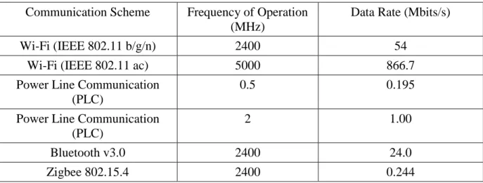
Table 1.2: Data rates of popular communication schemes Communication Scheme Frequency of Operation
(MHz)
Data Rate (Mbits/s)
Wi-Fi (IEEE 802.11 b/g/n) 2400 54
Wi-Fi (IEEE 802.11 ac) 5000 866.7
Power Line Communication (PLC)
0.5 0.195
Power Line Communication (PLC)
2 1.00
Bluetooth v3.0 2400 24.0
Zigbee 802.15.4 2400 0.244
Table 1.2 shows the data rates for some of the popular data communication technologies. The comparison of required data rate of power meters with Table 1.2 shows that required data rates can be provided by Wi-Fi, Bluetooth and PLC with 2 MHz bandwidth. Bluetooth is not viable because the data server for power meters is not in line of sight with the sensor nodes in
17
practical implementations and the distance between the sensor and data server usually exceeds the 1 m Bluetooth maximum theoretical range [1.13].
Wi-Fi technology is also not appropriate for the implementation of smart meters. Deployment costs for Wi-Fi nodes are low because Wi-Fi networks are popular and have penetrated most housing, industrial and organizational facilities. However, deployment of power meter nodes under the umbrella of existing Wi-Fi networks brings up administrative issues for common wireless channels with existing applications. In addition, Wi-Fi cards for embedded system applications are relatively costly [1.14].
Zigbee offers a great solution as the price of a 2.4 GHz radio from Digi International is $9-$15 [1.15] which is far less expensive than most of the current Wi-Fi transceivers in the market. The maximum range of a 2.4 GHz Zigbee transceiver is 90m, which is adequate for many building applications. In addition to Zigbee, IEEE 802.15.4 defines several schemes by which the Zigbee range can be increased. Schemes include recommendation to use intermediate devices called Zigbee routers which act as data concentrators collecting data from sensors. It is necessary to consider increased network latency and data rate restrictions of this type of multi-hop Zigbee network.
The restrictions in the bandwidth of Zigbee can be addressed by using a suitable data compression technique [1.16] to reduce the required data rate (described in Section 1.4.3). The data compression techniques are broadly classified into – Lossless and Lossy. Lossy data compression schemes (Example – JPEG and MPEG) are used in audio and video data compression. By comparison, the modern and efficient lossless data compression techniques use probabilistic models which are computationally intensive [1.18].
18
A simple method which demands less calculation is selected for the smart power meter. The power meter produces output of real power, reactive power, VRMS and IRMS. These values are produced every 1/60th of second. These results are q15 fixed point numbers. The compression technique, Run Length Encoding (RLE) reduces the redundancy in the data points. For example, reactive power values of 100 watts, 100 watts, 100 watts can be compressed to one value. This is a basic example of run-length encoding. RLE encodes to match a pre-defined value or the values which are repeated. Noise in monitored electric lines causes fluctuation in the power measured by the power meter. Thus a dead banding is introduced to improve compression technique. In this technique, the values are not transmitted if the corresponding value after comparison with the value last transmitted is in the dead band. This compression technique comes with a cost that signal changes in the dead band are lost. These changes are assumed to be due to the noise component in the monitored signal.
1.7 Hardware Platform of Smart Power Meter
The proposed smart meter has computationally intensive features which demand a microcontroller with good performance. However, performance of the smart power meter must be balanced against cost constrains. The important and non-compromising features considered in the microcontroller selection are memory and operating frequency. The memory of the microcontroller is vital for pattern matching and condition monitoring features as they require temporary storage of some of the associated parameters which are discussed in Section 1.4.2. The operating frequency is vital as it decides the upper cap of the total number of computations which can be performed by the microcontroller. The price of a microcontroller heavily depends on the above factors. Other features of the microcontroller are GPIO (General Purpose
Input-19
Output) pins, hardware timers, and advanced I/O capabilities, such as USB, that are fairly common across available microcontroller options.
1.8 Smart Power Meter – Architecture
Real Power Reactive Power RMS Voltage RMS Current DFT Results ADC HANDLER STAGE1 Data Pre-Processing DATA From Current Transformer and Voltage Sensing Board
STAGE2 Calculations
STAGE3
Radio Pre-Processing TO SERVER
Figure 1.6: Smart Power Meter – Software Architecture
Inside smart power meter node, analog data from voltage and current sensors are sampled by Analog to Digital Converters (ADC). The sampled data is stored in a buffer. Two buffers are used in the microcontroller and they are used alternatively. The digital data is processed as follows:
1.8.1 Stage 1
The data from ADC buffer is transferred to stage 1. The data from ADC is interleaved data which contains data from 15 channels. Stage 1 performs the function of un-interleaving data and converting data into q15 fixed-point format. The un-interleaved data is arranged into 2D matrix. The columns represent the channel and rows represent the type of measured parameter.
20 1.8.2 Stage 2
Stage 2 calculates RMS voltage, RMS current, real power and reactive power from un-interleaved data. The data from stage 2 is a 2D matrix which contains the calculated results. The columns represent the type of data and rows represent channels. Stage 2 also performs pattern matching and frequency scan and stores the results accordingly.
1.8.3 Stage 3
Stage 3 stores all results from stage 2 in a buffer. The data is subjected to Run Length Encoding (RLE) described in Section 1.6. The resulting data is transferred into the radio buffer when the buffer allocated to stage 3 is full.
1.9 Component Decisions for Smart Power Meter
The computational and communicational capabilities of the proposed smart power meter are discussed in Sections 1.5 and 1.6. Due to cost constrains in this project, communication bandwidth is constrained to 250 kBits per second. The product development team selected ATMEL SAM3SD8 processor which promises a clock frequency of 64 MHz and a flash memory of 512 Kbytes. The features of the microcontroller also include 64 Kbytes of SRAM memory with 79 GPIO (General Purpose Input-Output) pins. The team also has selected Zigbee radio to satisfy the bandwidth requirements of the smart power meters. The performance analysis of the same is discussed in Chapter 2 and Chapter 5.
1.10 Thesis Overview
This thesis covers a series of experiments and modeling steps to develop the smart power meter by optimizing the computational and communication bandwidth required for features in Section 1.4.
21
Chapter 2 explains an experiment conducted for performance analysis of communication in Zigbee network. Chapter 3 discusses an approach to improving the frequency response of the power meter by oversampling and then downsampling measurements in the analog front end and subsequent signal processing. Chapter 4 discusses a system level model developed in Simulink to measure computational performance characteristics of the selected ATMEL SAM3S based processor after implementation of smart power meter features discussed in Section 1.4.2. Chapter 5 discusses the communication performance of a network of the proposed wireless smart power meters.
22 1.11 References
[1.1] “Monitoring Energy Use: The Power of Information” [Online]. Available:
http://www.schneider-electric.com/solutions/ww/en/med/4665025/application/pdf/1256_monitoring_energy_use.pdf. [Accessed: 09-Dec-2013].
[1.2] “Guide to Energy Monitoring.” [Online]. Available: http://efergy.com/us/guide-energy-monitoring/. [Accessed: 10-Dec-2013].
[1.3] “An Overview of Energy Use and Energy Efficiency Oppurtunities.” [Online]. Available: http://www.energystar.gov/ia/business/challenge/learn_more/Schools.pdf .[Accessed: 10-Dec-2013].
[1.4] “Big Savings for Texas City with Energy Monitoring Sensors,” Energy.gov. [Online]. Available: http://energy.gov/articles/big-savings-texas-city-energy-monitoring-sensors. [Accessed: 10-Dec-2013].
[1.5] “Wattson: Monitor Your Home’s Energy Usage,” TreeHugger. [Online]. Available: http://www.treehugger.com/clean-technology/wattson-monitor-your-homes-energy-usage.html. [Accessed: 10-Dec-2013].
[1.6] J. Li, M. Sumner, J. Arellano-Padilla, and G. Asher, “Operating limits for drive condition monitoring using supply current signature analysis,” in Electric Machines Drives Conference
(IEMDC), 2011 IEEE International, 2011, pp. 412–417.
[1.7] “Quadlogic Power Meter - Low Cost, Accurate, Utility-Grade Electric Submeters, Tenant Billing.” [Online]. Available: http://www.quadlogic.com/products.html. [Accessed: 11-Dec-2013].
23
[1.8] “Power Xpert Meter 4000/6000/8000.” [Online]. Available:
http://www.eaton.com/Eaton/ProductsServices/Electrical/ProductsandServices/PowerQualityand Monitoring/PowerandEnergyMeters/PowerXpertMeter400060008000/index.htm. [Accessed: 11-Dec-2013].
[1.9] “Smart Meter, Dumb Idea?” [Online]. Available:
http://online.wsj.com/news/articles/SB124050416142448555. [Accessed: 11-Dec-2013]. [1.10] “PQMII Power Quality Meter.” [Online]. Available:
http://www.gedigitalenergy.com/multilin/catalog/pqmii.htm. [Accessed: 11-Dec-2013]. ASD
[1.11] “ATSAM3SD8C.” [Online]. Available: http://www.atmel.com/devices/SAM3SD8C.aspx. [Accessed: 11-Dec-2013].
[1.12] “IEEE Standard Definitions for the Measurement of Electric Power Quantities Under Sinusoidal, Nonsinusoidal, Balanced, or Unbalanced Conditions,” IEEE Std 1459-2010 (Revision
of IEEE Std 1459-2000), pp. 1–50, 2010.
[1.13] “Bluetooth - Wikipedia, the free encyclopedia.” [Online]. Available: http://en.wikipedia.org/wiki/Bluetooth. [Accessed: 12-Dec-2013].
[1.14] “Digi Connect Wi-Wave - 802.11b/g radio card for embedded system - Digi
International.” [Online]. Available: https://www.digi.com/products/wireless-wired-embedded-solutions/satellite-wifi-cryptographic/wifi-connectivity/digi-connect-wi-wave. [Accessed: 12-Dec-2013].
[1.15] “DigiKey Electronics - Electronic Components Distributor.” [Online]. Available: http://www.digikey.com/. [Accessed: 12-Dec-2013].
24
[1.17] “Run-Length Encoding.” [Online]. Available: http://www.dspguide.com/ch27/2.htm. [Accessed: 09-Dec-2013].
[1.18] “Burrows-Wheeler Transform” [Online]. Available:
http://www.cs.cmu.edu/~ckingsf/bioinfo-lectures/bwt.pdf. [Accessed: 09-Dec-2013].
[1.19] Matt O’Connell, M.S. thesis (Under preparation), ME Dept., Colorado State University, Fort Collins, CO, 2014.
[1.20] “Basic kWh Meter 100A 120/240-volt, 3-wire, 60Hz EKM-25IDS.” [Online]. Available: http://www.ekmmetering.com/ekm-metering-products/electric-meters-kwh-meters/basic-kwh-
meter-100a-120-240-volt-3-wire-60hz-ekm-25ids.html?gclid=CIi8gZ-QuLsCFcsRMwod_nAAGQ. [Accessed: 17-Dec-2013].
[1.21] “SiteStage Features” [Online]. Available: http://powerhousedynamics.com/about-sitesage/features1. [Accessed: 04-May-2014]
[1.22] “SiteStage Energy Monitor” [Online]. Available: http://www.amazon.com/SiteSage-24h-formerly-eMonitor4-24-Powerhouse-Dynamics/dp/B006Z5OKW8. [Accessed: 04-May-2014]
25 Chapter 2
Zigbee Radio Range Testing 2 Overview
This chapter describes an experiment performed to measure the performance of Zigbee network in a test environment where the proposed smart power meter will be deployed. Section 2.1 introduces the Zigbee protocol with a comparison of Zigbee protocol with the popular communication protocols in the current market. This section also introduces the co-existence of Wi-Fi with Zigbee schemes.
Section 2.2 explains test setup to measure the performance of Zigbee based wireless communication in a clean environment and an environment with several Wi-Fi radios. The Data Loss is selected as a metric to measure the performance. Section 2.3 presents the results of the test.
2.1 Introduction
Since its invention, Zigbee has aimed in devices such as switches, energy meters and sensor systems functioning in commercial and industrial buildings which were overlooked by wireless radio industries. Zigbee alliance members created a wireless standard offering easy installation and a mechanism for coexistence of Zigbee with other wireless systems working in the same operation frequency of Zigbee devices. Zigbee is built using the Institute of Electrical and Electronics Engineers (IEEE) 802.15.4 [2.11]. Though low powered, Zigbee devices can achieve long distances by passing data through intermediate Zigbee radios, forming a mesh network. The Zigbee networks are secured by 128 bit encryption keys. Zigbee communication protocol claims to achieve data transmission rates of up to 250Kilobits per second when operating in the frequency of 2.4 GHz.
26
Zigbee is primarily used in applications which require a low data rate, prolonged battery life and a secure network. The Zigbee protocol supports star, mesh and tree type networks. Every Zigbee network has a coordinator node which is responsible for control of network parameters and basic maintenance of network.
2.1.1 Zigbee Protocol Stack
The Zigbee protocol stack is based on IEEE 802.15.4 standard [2.11]. This standard gives special emphasis for low cost communication with no underlying infrastructure so that users can exploit this to achieve lowest power consumption demanded by their respective application. The main features of IEEE 802.15.4 are real-time reservation of time slots for transmission nodes and collision avoidance through CSMA/CA. Features also include functions for smart power management in Zigbee radios.
Medium Access Control
Physical Layers IEEE 802.2 Logical Link Control
Convergence Sublayer Upper Layer
27
IEEE has defined only lower layers of OSI model in IEEE 802.15.4 standard. Protocols for the transfer of data to and from upper layer are defined in IEEE 802.2 standard. The lower physical layer performs channel selection and energy management functions. The MAC layer enables the transmission of data frames from application layer to physical layer. The MAC layer also performs functions such as network beaconing, time slot reservation and frame validation. 2.1.2 Zigbee Frequency of Operation
Zigbee operates in license-free Industrial, Medical and Scientific (ISM) band. Zigbee operates in three ISM bands – 2.4 GHz (Worldwide), 915 MHz (North America and Australia) and 868 MHz (Europe).
2.1.3 Zigbee Range Comparison
Table 2.1: Zigbee Comparison with Wireless Standards [2.5] Zigbee 802.11 Bluetooth Ultra- Wide
Band Wireless USB Data Rate 250 Kb/s 11/54 MB/s 1 Mb/s 100-500 Mb/s 63 Kb/s Range 10-100 meters 50-100 meters
10 meters 0-10 meters 10 meters Network Topologies Supported Peer to peer, ad-hoc, star and mesh Point to hub, ad-hoc Point to point Point to point Point to point Operating Frequency 2.4 GHz (Worldwide) 2.4 GHz and 5 GHz 2.4 GHz 3.1 to 10.6 GHz 2.4 GHz Power Consumption
Low High High Low Low
Security 128 AES None 64 and 128
bit encryption
None None
Table 2.1 and Figure 2.2 presents a comparison of popular wireless Personal Area Networks (PAN) networks in terms of data rate, range, network topologies, operating frequency, power consumption and security features. Zigbee offers data rates of 250 Kbits per second while
28
Wi-Fi promises more than 10 times the bandwidth and range of Zigbee. Bluetooth promises higher data rate but lesser range compared to Zigbee.
0.01 0.1 1 10 100 1000 Zigbee Bluetooth IEEE 802.22 IEEE 802.20 WiMax 802.15.3 Data Rate (Mbps) Range WIFI
Figure 2.2: Zigbee Protocol Comparison (Range Vs. Data Rate) [2.5]
Section 1.6 described communication schemes and the practicality of using these schemes with the smart power meter. The choice of wireless communication technology for the smart power meter was narrowed down to Zigbee or Wi-Fi in Section 1.6. Wi-Fi has a data rate almost 1000 times more than Zigbee. Wi-Fi also has better range compared to Zigbee. The Zigbee scheme is selected because Zigbee transceivers are priced less than Wi-Fi transceivers and they are within the project budget. The IEEE 802.15.4 standard recommends schemes to increase the range by using intermediate device called Zigbee routers. The router also helps to control the data flow in the network by buffering the data from the sensor nodes.
29 2.1.4 Coexistence with Wi-Fi
The Zigbee operates in license-free industrial scientific and medical (ISM) bands. The following wireless systems are the main users of 2.4 GHz ISM band:
802.11 b/g/n networks Bluetooth networks Cordless phones Microwave Ovens WiMax Systems
The Zigbee radio, which operates in the frequency of 2.4 GHz, shares its frequency of operation with the above wireless systems and hence they are susceptible to interference from other wireless systems. The table below shows the wireless channels of operation of Zigbee radios as specified in IEEE 802.15.4 when they are operated in the frequency of 2.4 GHz.
30
Table 2.2: Zigbee Channels [2.6]
Channel No Center Frequency (GHz)
11 2.405 12 2.410 13 2.415 14 2.420 15 2.425 16 2.430 17 2.435 18 2.440 19 2.445 20 2.450 21 2.455 22 2.460 23 2.465 24 2.470 25 2.475 26 2.480
The main source of interference for Zigbee signals are Wi-Fi signals. Wi-Fi signals are the most dominant contributor of interference compared to other wireless technology working in the same operational frequency. This is due to the high penetration of Wi-Fi networks in
31
commercial and residential applications. This penetration causes significant Wi-Fi network traffic in industrial, commercial and housing establishments which can interfere with Zigbee transmissions operating in the same frequency. The Wi-Fi devices used in US operate in 11 wireless channels in 2.4 GHz band. Each channel is evenly spaced at 5 MHz separation. Channel 1 operates at 2.412 GHz and channel 11 operates at 2.462 GHz. Wi-Fi protocol also demands a channel separation of 16.25 MHz to 22 MHz between its channels. Wi-Fi communication channels overlaps with the channels allocated for 802.15.4 protocol. This can reduce the performance of Zigbee radio as Zigbee operates in much lower power compared to Wi-Fi systems (WIFI signals are transmitted at 1 watt [2.7] compared to Zigbee pro which transmits at 63 mW [2.3]).
The performance of wireless power meters depends on existing Wi-Fi networks in the environment. Zigbee signals can also interfere with cordless phone and Bluetooth network signals which are operating in 2.4 GHz bandwidth. The measurement of performance is necessary before the deployment of sensor nodes to make necessary changes to architecture and the transmission time of the nodes.
2.2 Test Setup – Zigbee Performance Measurement
Packet loss was selected as the metric to measure the performance of the Zigbee network. Two Zigbee nodes were used in the test – One was configured as a client (Zigbee end device) and other as server. Packets were transmitted from the client to server. The test was conducted with Regular Zigbee Radio (900 MHz bandwidth, 10mW transmission power) and Pro Zigbee Radio (2.4 GHz bandwidth, 63mW transmission power). The effect of processor power (Clock frequency of the processor) to process the received data is also investigated by using Zigbee radios with a personal computer ( 2GHz clock frequency Intel Celeron processor) and with an
32
Arduino board (16MHz microcontroller clock frequency). The test was also conducted in two environments – Wi-Fi environment and Non Wi-Fi environment to characterize the effects of Wi-Fi devices in the operating environment.
The data packets were generated in client. Each data packet consists of a time stamp, network address, source address, packet length, protocol version, counter (incremented with each packet as generated by the client), device time stamp and receive time stamp. The receiver Zigbee node monitored the counter values to detect data loss. Time stamps were used to estimate delay in data.
Figure 2.3: Zigbee Performance Test Setup
The test was performed in Engines and Energy Conversion Laboratory (EECL) at Colorado State University (Wi-Fi environment) and at City Park, Fort Collins (Non Wi-Fi environment). EECL had 3 WIFI networks. In the Wi-Fi environment, traffic was highest in Colorado State University Wi-Fi network (Center Frequency at 2.422 GHz). The Zigbee nodes
33
were configured to operate in channel 14 (Center frequency at 2.420 GHz). This channel was selected to measure the performance of the network when the Zigbee radios operate in the same frequency as Wi-Fi radios.
2.2.1 Experiment 1
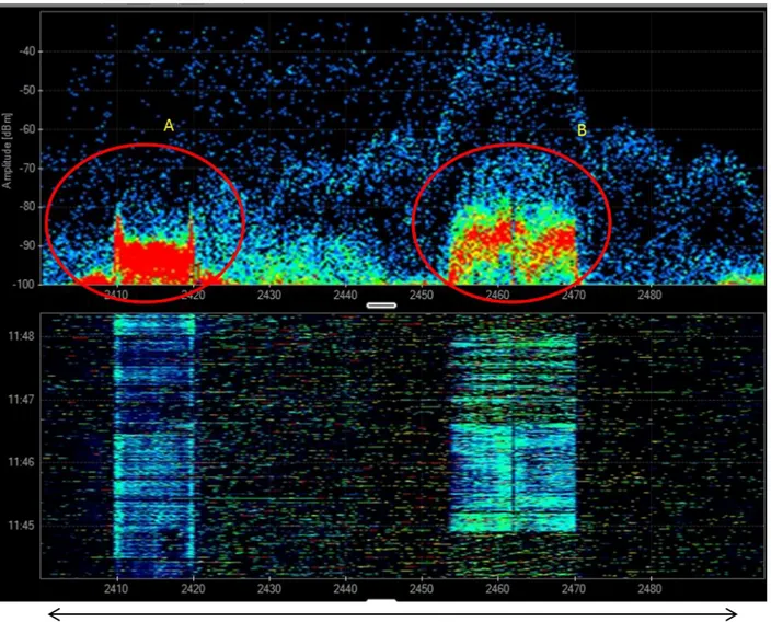
The experiment was performed in Engines and Energy Conversion Lab at CSU. Figure 2.4 and Figure 2.5 shows the screenshot of 2.4 GHz spectrum recorded by channel analyzer. The top half of the diagram shows discrete plots of signal energy and bottom half shows a flow diagram in which amplitude (X-Axis) is plotted with time (Y-Axis). The color of the dots in plot depicts the intensity of signal in the frequency band. In Figure 2.4, A and B shows the frequency range where high power Wi-Fi transmission is recorded. These Zigbee radios are operated in this frequency band as described in Section 2.2.
Spectrum recordings of the 2.4 GHz spectrum showed significant wireless activity in Wi-Fi channel 2 (2.410 GHz), channel 3 (2.415 GHz) and channel 4(2.420 GHz). The Zigbee radio was operated in channel 13 (2.415 GHz). The test was performed with two configurations: UART connection between Zigbee receiver and PC (INTEL processor with 2.4 GHz)
which records the received data.
The received data was processed by Arduino stalker (ATMega328P microcontroller with 20 MHz).
The test was performed in two configurations to quantize the effect of clock frequency of the chip responsible for transmitting/receiving data by using Zigbee radios in the test environment. The test was also performed with regular Zigbee (900 MHz) and pro-Zigbee (2.4 GHz) to quantify the effect of frequency of operation of Zigbee radios.
34
Figure 2.4: 2.4 GHz Spectrum (WIFI Environment) 2.2.2 Experiment 2
In experiment 2, all radio parameters were the same as experiment 1. The experiment 2 was conducted in an environment without Wi-Fi signals. Figure 2.5 shows 2.4 GHz spectrum in the scenario. The scenario showed no wireless signal activity in 2.4 GHz spectrum.
35
36 2.3 Test Results
Figure 2.6: Zigbee Radio Performance with WIFI Interference (Packet Loss Vs. Distance (meters))
37
Figure 2.7: Zigbee Radio Performance in Environment Without WIFI (Packet Loss Vs. Distance (meters))
Figure 2.6 and Figure 2.7 show the performance of Zigbee radios working in an environment with Wi-Fi signals and without Wi-Fi signals. The comparison between Figure 2.6 and Figure 2.7 shows that Zigbee radios used with Arduino based processors perform better in terms of range in an environment without Wi-Fi. The test results show that when the Zigbee radio is used in Arduino board with an ATMEL microcontroller (ATMega328P), their range is limited to 30m (900 MHz Zigbee radio). In an environment with Wi-Fi activity (Figure 2.6), the Zigbee shows a performance improvement when used with a faster processor (The range is improved to 70m). Thus a faster backend processor in Zigbee end node improves the communication efficiency of Zigbee networks. The comparison of test results from experiments in Section 2.2.1 and Section 2.2.2 shows that in an environment with Wi-Fi, the packet loss
38
reaches 100% at 35 meters whereas the same radios when used in environment without Wi-Fi the 100% packet loss is recorded at 45 meters. Therefore, the performances of Zigbee modules are limited by Wi-Fi signals in the environment. In Figure 2.6, the comparison between performance of Zigbee radio used with Arduino boards (Blue bar) and Zigbee radio used with Intel processor connected via UART (Yellow bar) shows that the Zigbee radio used with an Intel processor shows a packet loss of 60% at 55 meters and the Zigbee radio with Arduino based processor showed a 100% loss of packets at 55 meters. Therefore, performance of Zigbee radio is also limited by type of processor used with Zigbee modules.
2.4 Conclusion
The performance test results reveal that Zigbee module performance is significantly limited when they operate in channels which overlap with Wi-Fi channels operating in the same frequency. The recorded range is much less than the range predicted by Digi International, the developer of the Zigbee modules utilized here. Digi International states that range for 900 MHz and 2.4 GHz Zigbee radio are 610m [2.8] and 90m [2.9] respectively. It is recommended that Zigbee channels are selected by considering existing WIFI networks in the deployment environment.
The packet loss in Zigbee based communication can also be due to ground reflection [2.10]. Ground reflected signals can play a prominent role in performance of low power devices. The wireless signals also reflect from PCB (Printed Circuit Board) where Zigbee radios are mounted. The Figure 2.8 shows Arduino board with Zigbee radio mounting pins. In this board, the mounted Zigbee radio is only few inches above PCB board which increases the reflected wireless signals from the board.
39
Figure 2.8: Example of PCB board with Zigbee radio mounting pins
Performance degradation due to ground based reflection can be avoided by design improvements in the system. One of suggested improvements is to place the radio in an independent PCB and place it higher or at a distance with respect to PCB board containing microcontroller and other circuitry. This will reduce the reflection of Zigbee radio signals from the circuit board.
40 Processor/Micro-controller with transducer Zigbee Radio Ground Level D at a F lo w D m et er s
41 2.5 References
[2.1] “Zigbee”, [Online], Available: http://en.wikipedia.org/wiki/Zigbee, Last Accessed: 11/07/2013
[2.2] “Hirose U.FL”, [Online], Available: http://en.wikipedia.org/wiki/Hirose_U.FL, Last Accessed: 11/07/2013
[2.3] “Xbee 802.15.4”, [Online], Available: http://www.digi.com/products/wireless-wired-embedded-solutions/Zigbee-rf-modules/Zigbee-mesh-module/ , Last Accessed: 11/07/2013 [2.4] “Zigbee and Wireless Radio Frequency Coexistence”, [Online], Available:
https://docs.Zigbee.org/Zigbee-docs/dcn/07-5219.PDF, Last Accessed: 11/07/2013 [2.5] “How does Zigbee compare with other wireless standards?”, [Online], Available: http://www.stg.com/wireless/Zigbee_comp.html , Last Accessed: 11/07/2013
[2.6] “Zigbee Channels”, [Online], Available: http://www.metageek.net/control4/Zigbee-channels/, Last Accessed: 11/07/2013
[2.7] “FCC rules for operation in ISM bands”, [Online], Available: http://www.afar.net/tutorials/fcc-rules/, Last Accessed: 11/07/2013
[2.8] “Xbee-PRO 900HP”, [Online], Available: http://www.digi.com/products/wireless-wired-embedded-solutions/Zigbee-rf-modules/point-multipoint-rfmodules/xbee-pro-900hp#specs , Last Accessed: 11/08/2013
[2.9] “Xbee 802.15.4”, [Online], Available: http://www.digi.com/products/wireless-wired-embedded-solutions/Zigbee-rf-modules/point-multipoint-rfmodules/xbee-series1-module#specs, Available: 11/08/2013
42
[2.10] O. Musikanon and W. Chongburee, “Zigbee Propagations and Performance Analysis in Last Mile Network,” International Journal of Innovation, Management and Technology, vol. 3, no. 4, 2012.
[2.11] “IEEE Standard for Information Technology - Telecommunications and Information Exchange Between Systems - Local and Metropolitan Area Networks Specific Requirements Part 15.4: Wireless Medium Access Control (MAC) and Physical Layer (PHY) Specifications for Low-Rate Wireless Personal Area Networks (LR-WPANs),” IEEE Std 802.15.4-2003, pp. 0_1–670, 2003.
43 Chapter 3
Digital Filter Overhead Estimation 3 Overview
This chapter explains the estimation of computational overhead in the sampled data of the smart power meter. In the proposed smart power meter, Analog to Digital Converter (ADC) digitizes the analog data received from the voltage and current sensors. The ADC samples at a sampling rate which is almost 20 times Nyquist frequency. The high sampling frequency avoids aliasing and feeds high frequency data to algorithms. This sampling rate would demand a high computation power resource. Hence, a downsampling process is required before transferring the data into calculation stages described in Section 1.8. A typical downsampler system contains a digital low pass filter in the front-end to avoid effects of aliasing after the downsampling process. The implementation of digital filter requires a set of computation steps which depends on the type and number of poles of the filter. The computational load incurred by downsampling process depends upon the frequency of the data supplied to it. The computational load also depends on the type of arithmetic used for filter implementation. Thus, it is more efficient to do the downsampling of the data in stages. This chapter models the calculation of net computation overhead and overhead in each stage of downsampling process. This is followed by estimating the overhead for two proposed configurations.
3.1 Introduction
The implementation of filters in a microcontroller can be carried out in two ways – fixed point and floating point. The fundamental difference between these two is in their respective representation of numerical data.
44
The digital filters using floating point arithmetic to represent digital data offers much greater numerical bandwidth compared to the digital filters using fixed point arithmetic. However, floating point filters require complex computations compared to fixed point filters. Therefore, implementation of floating point filters typically require a microcontroller platform which has a built-in floating point unit to handle the complex floating point computations. This requirement can increase the component costs of the proposed smart power meter.
In order to understand the effect of the type of arithmetic on the performance of filters for the smart power meter, fixed and floating point capabilities are compared. In digital filters working in floating point arithmetic, each time a processor generates a new fixed point number, the number is rounded to nearest value so that number can be stored in a defined number of bits. Rounding and truncating noise are introduced in the signal which leads to significant deviation between the theoretically correct result and results produced by the software implementation of the smart power meter. Typically, this deviation is much larger in fixed point than in floating point systems.
3.1.1 Factors to Consider for Filter Selection
The following are the key factors to consider before selection of fixed point or floating point based implementation [3.2]:
Processor Cost: The ability to lower cost can significantly impact product profitability.
Fixed point computations can be performed on microcontrollers without floating point units (FPU) or co-processors, and are typically less expensive than microcontrollers with floating point capability.
Ease of Development: The easier the development, the faster the product can be released
45
consideration of round-off errors in accumulators and similar software features. Fixed point algorithms must often be modified significantly from “textbook descriptions” to avoid truncation errors. The additional algorithmic development effort can make fixed-point development significantly more expensive.
Performance: The performance is a metric which shows the speed with which the tasks
are performed by the processor. This metric largely depends on processor in the application. It is possible to use fixed point algorithm in a floating point processor and vice versa.
3.1.2 Implementation in Smart Power Meter
Analog Front End Board
Analog to Digital Converter
Downsampler Algorithm
Figure 3.1: Front End System of Data Flow
The data from the analog sensors which capture voltage and current signals are sent to the Analog to Digital Converters (ADC) in the smart power meter. The ADC samples the data at frequencies much higher than the Nyquist limit to avoid aliasing. Directly processing this high frequency data would be computationally intensive and hence downsampling is used to lower the frequency of data before the data is processed by the algorithms in the smart power meter. This
46
downsampling process should designed to avoid loss of the key signal components required for the algorithms implemented in the proposed smart power meter.
3.1.2.1 Downsampling
Low Pass Filter Downsampler
Figure 3.2: A Typical Downsampler
Downsampling is a process of reducing the sampling rate of a signal. The extent of downsampling called downsampling factor should be an integer greater than unity. As an example, if a signal sampled at 2 KHz is downsampled at 1 KHz; the signal is downsampled by a factor of 2. The downsampling factor is denoted by letter M.
In the implementation of downsampler, care should be taken to avoid aliasing. The frequency of signal fed into downsampler should be limited to 𝑓𝑠
2𝑚 where 𝑓𝑠 is the frequency of the baseband signal. The more the signals spectrum contains signal components whose frequency is greater than2𝑚𝑓𝑠, the greater the extent of aliasing. Hence, the implementation of a downsampler requires a low pass filter implemented in its front- end to remove the signal components greater than 2𝑚𝑓𝑠 where 𝑓𝑠 is the frequency of the sampled signal.
47
The downsampling of frequencies can be done in single stage or multiple stages. Multi-stage downsampling has an advantage that higher-frequency signals can be routed accordingly to the algorithms requiring higher frequency data, while other algorithms can receive lower-frequency signals tapped from the respective stage of downsampling. Multi-stage downsampling can also reduce the computational overhead because the computational load required by a particular stage depends on the sampling frequency of input data to that stage. A higher order downsampler requires Low Pass Filter (LPF) with sharp cut-off frequency to avoid aliasing. The roll-off of the cut off frequency in the designed LPF depends on the number of poles of the filter. Increasing the number of poles increases the number of multiplication and additions per input sample. Hence, it is computationally efficient to implement the downsampling process in stages where the stages with lower downsampling factors are subjected to high frequency data and the lower frequency data from it are subjected to downsamplers with higher downsampling factors.
In a multi-stage downsampler (Figure 3.3), the multiple downsamplers (D1,D2 ,.. Dn) are used to reduce the frequency of the data before the data is sent to computational algorithms (discussed in Section 1.4). The input to D1 is at the highest frequency and is more computational intensive than D2, which receives downsampled data from 𝐷1 at a lower frequency. Therefore, the analysis of computations in the proposed architecture of downsampler is necessary to estimate the computations needed in every section of design. This approach can also help in better implementation of algorithms. As an example, the condition monitoring process described in Section 1.4.4 uses Discrete Fourier Transforms (DFT) and the resolution of the signal by the DFT depends on the sampling frequency of the signal.
The Infinite Impulse response (IIR) filter was selected to implement the downsampler as it takes lesser memory than Finite Impulse Response filter. An IIR filter requires fewer


![Figure 2.1: IEEE 802.15.4 Protocol Stack [2.1]](https://thumb-eu.123doks.com/thumbv2/5dokorg/5519840.143984/38.918.233.684.565.983/figure-ieee-protocol-stack.webp)
![Figure 2.2: Zigbee Protocol Comparison (Range Vs. Data Rate) [2.5]](https://thumb-eu.123doks.com/thumbv2/5dokorg/5519840.143984/40.918.160.765.198.616/figure-zigbee-protocol-comparison-range-vs-data-rate.webp)