Aerodynamics of Bird Flight

(1)

AERODYNAMICS OF BIRD FLIGHT

AISHWAR RAVICHANDRAN

921015-T115

Degree Project in Vehicle Engineering

Stockholm, Sweden 2014

(2)

ACKNOWLEDGEMENT

Firstly, I would like to thank my guide Professor Luca Brandt for guiding me throughout the course of this project and providing relentless support. It has been a really fascinating experience that has given me lot of knowledge.

I would also like to thank my parents for their support. It is their love and affection that has driven me throughout.

(3)

ABSTRACT

It is the objective of this thesis project to understand the physics behind the different modes of bird flight and to do numerical two dimensional simulations of pure plunging, pure pitching and combined pitch-plunging motion of an aerofoil. First, the different physical models used to understand the generation of thrust are explained. Then the numerical model used for the simulation is explained briefly. Then the results and analysis of the numerical simulations are presented.

(4)

Chapter 1 Introduction

Humans have been fascinated by ability of birds and insects to fly and have always wanted to replicate these creatures to earn their rightful place among them in the sky. Over the years there have been many scientists who have tried to understand these marvels of nature. The most famous among them was the 'artista', Leonardo di ser Piero da Vinci; in the year 1485 he designed a flapping wing aircraft after doing through research on the birds.

Birds and insects flap their wings to generate thrust and lift, and also perform remarkable manoeuvres. These provide us with fascinating and illuminating examples of unsteady aerodynamics. Additional interest in aerodynamics of flapping animals has been due to the development of micro air vehicles. It is important to understand the flapping mechanisms used in nature in order to adopt or modify them to design flapping wing vehicles. To this end, it is necessary to provide the engineers with the aerodynamic knowledge required to select the most suitable flapping mechanism for the given mission objectives.

1.1 LITERATURE REVIEW

J. D. Delaurier [6] developed an aerodynamic model for flapping wind model to predict the lift, drag etc.

Taylor et al. [3] analyzed the amplitudes and frequency of flapping of 42 species of birds, bats, and insects in cruise flight. He found that the dimensionless Strouhal number, the dimensionless flapping frequency, was a useful similarity parameter.

Katzmayr [7] studied the effects of a sinusoidally oscillating air stream on a stationary wing. This was the first experimental verification of the Knoller–Betz effect described in chapter 2.

von Kármán and Burgers [8] explained the production of thrust by oscillating aerofoils based on the position and orientation of the vortices in the wake.

Theodorsen [9] derived the solution for an incompressible flow past an oscillating aerofoil. He found that the reduced frequency was the correct parameter to measure the unsteadiness of a flow.

Garrick [4] predicted the thrust and the propulsive efficiency of plunging and pitching aerofoil. Like Theodorsen, he assumed the all the motions to be harmonic.

(7)

2 Jones et al. [10] measured (using laser-Doppler velocimetry) and studied the velocity profile of the wake of an pure plunging wing.

Lai and Platzer [11] studied the characteristics of the jet like profile produced by plunging motion. Young [2], Lai [11] and Heathcote [12] published results of experiments done on a plunging NACA0012 aerofoil.

Max F. Platzer, Kevin D. Jones et.al. [5] reviewed the recent developments in the understanding of aerodynamics of flapping motion.

1.2 Objectives

• To understand bird flight and the different theories used to explain its aerodynamics. • Perform numerical simulation of pure plunging, pure pitching and combined

pitch-plunging motion of an airfoil and analyse the results.

1.3 OUTLINE OF CHAPTERS

In Chapter 2 we first explain the different modes of flight in nature. Then different physical theories used to explain the aerodynamics of oscillating aerofoils are explained.

In Chapter 3 we give the results of the simulations done on pure pitching, pure plunging and combined pitching and plunging motion of NACA 0012 aerofoil. The conclusions drawn from these numerical analysis is also presented.

(8)

3

Chapter 2 Theoretical background

In this chapter we shall introduce the main concepts to understand the forces acting on a wing and how these are used in nature for animal flight.

2.1 Aerodynamic forces

Aerodynamic forces are exchanged between a body and a fluid surrounding it, and are due to the relative motion between the body and the gas. In the case of an aerofoil or a wing these forces are resolved into two components : Lift and Drag.

Figure 1: Aerodynamic forces on an aerofoil

Lift

Lift is the component of the aerodynamics force perpendicular to the flow direction. The explanation for the generation of lift is based on the Newton's second and third laws of motion: The net force on an object is equal to its rate of momentum change, and: To every action there is an equal and opposite reaction.

An aerofoil deflects the air as it passes the airfoil. As the aerofoil must exert a force on the air to change its direction, the air must exert a force of equal magnitude but opposite direction on the aerofoil. A wing, non symmetric or with the appropriate angleof attack, exerts a

(9)

4

downward force on the air and thus the air exerts an upward force on the wing. Lift is a reaction force. A net force also indicates the presence of a pressure difference. The direction of the force, let us assume upwards, indicates that the average pressure on the lower surface of the aerofoil is larger than the average pressure on the upper surface of the aerofoil.

Drag

Drag refers to forces acting opposite to the relative motion of any object moving with respect to a surrounding fluid. This can exist between two fluid layers or a fluid and a solid surface. Unlike other resistive forces, such as dry friction, which are nearly independent of velocity, drag forces depend on velocity. Drag always works to decrease the fluid velocity relative to the solid object in the path of the fluid.

Angle of attack

It is the s the angle between the body's reference line (cord in the case of an aerofoil) and the direction of the oncoming flow.

Figure 2: Angle of attack

A symmetrical airfoil generates zero lift at zero angle of attack. As the angle of attack increases, air is deflected through a larger angle and the vertical component of the velocity of the air, that will be deflected by the rigid body, increases resulting in increased lift.

(10)

5

2.2 Flight modes in nature

Animal flight in nature can be divided into two modes: unpowered (gliding and soaring) and powered (flapping).

Unpowered flight

Gliding

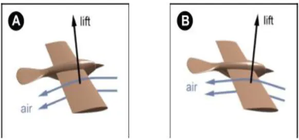
Birds flap their wings to generate lift and thrust. When they stop flapping and keep their wings stretched out, the wings actively produce lift (a vertical force sustaining them), not thrust (force in the direction of motion). A component of the gravity force in the direction of flight of a descending bird can as act as thrust. This mode of flight is called gliding. Birds like vultures, albatrosses and storks are great gliders as they have very high lift to drag ratio. Bird with large wing have evolved to become gliders as they have very high aspect ratios, which also means that they have very high lift to drag ratio. Some fishes, amphibians, reptiles, and mammals have also evolved to become gliders.

A bird has to produce both lift and thrust to counteract gravity and drag, and to maintain flight at a certain level. As there is no active thrust generation during gliding birds use the gravity to counteract the drag. To achieve this birds tilt their direction of motion downward relative to the direction of incoming air. This results in an angle between the direction of incoming air and the direction of motion. This angle is referred to as the glide angle. This angle has an inverse relationship with the lift to drag ratio. Higher the lift to drag ratio, smaller the glide angle. This ratio is also increasing with the Reynolds number, a fudamental non-dimensional parameter in fluid mechanics that is proportional to the velocity and the size of the bird.

[15] Figure 3: A) Bird in level flight , B) Bird in a shallow dive

(11)

6

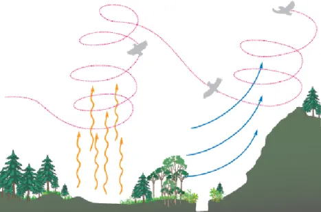
Gliding always results in the loss of altitude of birds. Birds resort to soaring to maintain or gain altitude. Soaring is special gliding mode in which the bird uses rising air currents instead of gravity. The energy required to sustain or increase the altitude is taken from the atmosphere.

[15] Figure 4: Soaring of birds

Powered flight : Flapping

Flapping, in contrast to gliding, involves the active production thrust by the wings. There are two stages in flapping: down stroke or power stroke, which produces a large proportion of the thrust, and upstroke or recovery stroke, which depending on the bird's wing produces some amount of lift. During the upstroke the wing is slight folded inward to reduce the upward resistance. The angle of attack of the wing is also changed for these strokes. It is increased for the down stoke and decreased for the upstroke.

As the wing is flapping, it also moving forward through the air along with the body of the bird. The amplitude of the up and down movement is very small close to the body. But towards the wingtip the amplitude is much higher. As a correct angle of attack has to be maintained throughout the wing, the birds resort to twisting them. As the wing is twisted, the outer part of the wing moves downward, so the lift in this part is angled forward. This is similar to what happens when bird does a dive. But in this case only the wing moves downward and no the entire bird. The bird can therefore generate the required amount of thrust without losing altitude.

(12)

7

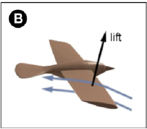
[15] Figure 5: A) Twisting of the wing , B) Shows the generation of lift and thrust during down stroke.

In the upstroke, the outer part of the wing points directly in the line of travel so that it produces very little resistance. The angle of attack is effectively reduced to zero. Bird also fold their wing to help in reducing the resistance. The wingtip features also separate creating natural slots that further reduce the resistance.

The inner part of the wing does not undergo much of a up and down motion, so it functions more or less as it would during gliding, i.e. generating lift continuously. As only the inner part of the wing produces lift during the upstroke, upstroke on the whole generates very little lift compared to the down stroke. As a result of this the bird slightly bobs up and down during the flight.

[15] Figure 6: A) the inner part of the wing produces lift in both the strokes. B) outer part of the wing passing through the air with zero angle of attack during the upstroke.

(13)

8

2.3 The Physics of Drag and Thrust Generation Due to aerofoil Flapping

Knoller-Betz effect

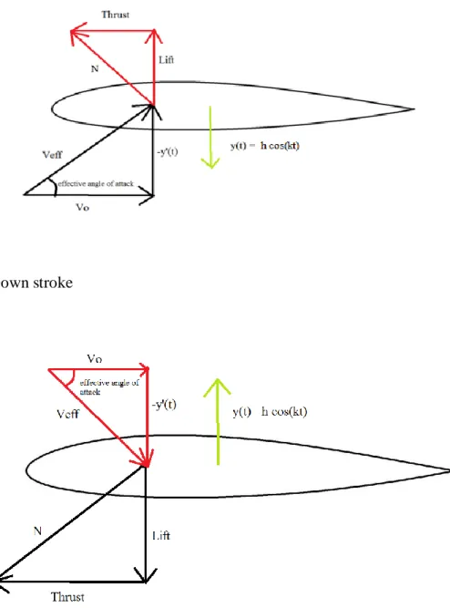
Knoller [13] and Betz [14] in their independent studies on pure heaving aerofoils perceived that a heaving aerofoil creates an effective angle of attack that generates an aerodynamic force, N, which decomposes into lift and thrust components. The following figures illustrates an aerofoil generating thrust and lift during down stroke and upstroke. Positive thrust is generated during both the stokes, yielding a positive time averaged thrust as a result of heaving.

Figure 7: Down stroke

(14)

9

Theoderson's theory

The theory developed by Theodorsen [9] was based on potential flow theory for the lift and pitching moment of a thin airfoil with a flap undergoing pitching and plunging motion. The theory assumes harmonic motion and small perturbations. An analytical solution was obtained which gave the loads on the airfoil in terms of the Theodorsen's function and kinematics. Theodorsen also showed that reduced frequency was the correct measure of the unsteadiness of the flow as the Theodorsen's function was solely a function of reduced frequency.

Inverse Karman vortex street

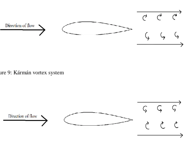
In 1935 von Kármán and Burgers [8] presented the first theoretical explanation for the production of thrust or drag based on the observed location and orientation of the vortices in the wake. When an aerofoil is oscillating (pitching/plunging or both combined), it can produce either of the two kinds of vortex system in its wake : Kármán vortex or inverse Kármán vortex. These two systems are shown in the following figures.

Figure 9: Kármán vortex system

Figure 10: Inverse Kármán vortex system

An aerofoil with Kármán vortex system in its wake produces drag and the one with inverse Kármán vortex system produces thrust. The upper row of vortices in the inverse Kármán

(15)

10

vortex system is anticlockwise and the lower row vortices are clockwise. Flow is obviosly being entrained between the two vortex rows such that the time-averaged velocity distribution in planes perpendicular to cord of the aerofoil is that of a jet profile. So the oscillating aerofoil produces a jet, as a reaction thrust is produced on the aerofoil.

Dynamic Stall and Leading Edge Vortex Shedding

Dynamic stall is a non-linear unsteady aerodynamic effect that occurs in an airfoils with rapidly changing angle of attack. Due to the rapid change in angle of attack a strong vortex is shed from the leading edge of the airfoil, and it travel backwards above the aerofoil, it strongly interacts with the trailing edge vortex. The vortex contains high velocity air particles which leads to a brief increase in the lift produced by the aerofoil. However there is rapid loss in the lift and changes in pitching moment as the vortex passes behind the trailing edge. This leads to a hysteresis loop in lift, drag and pitching moment .

(16)

11

Chapter 3 Numerical simulations

3.1 Introduction to CFD

During the last few decades, owing to the rapid development of desktop and large-scale computational resources, it became more and more common to use numerical simulations to reproduce virtual experiments, so called CFD (computational fluid mechanics). Numerical simulations can be cheaper than laboratory experiments, and enable us to extract all fluid flow quantities in time and space, also those usually not accessible from measurements. Simulations, however, are limited to low Reynolds number Re (low speeds) and the accuracy can be compromised by the models used to mimic the effect of turbulence at low resolutions.

3.2 Numerical code

All the simulations in this project were done using Ansys Fluent (version 6.1). Ansys Fluent software has broad physical modelling capabilities which allow it to model fluid flows, turbulence, heat transfer, and chemical reactions. It basically solves the Navier–Stokes equations numerically for the given problem.

Turbulence model

In Large eddy simulation technique the smallest scales of flow are ignored through a filtering operation, and the effects are modelled using subgrid scale models. The largest and most important scales of turbulence are resolved, while greatly reducing the computational cost. Spalart–Allmaras turbulence model was used for the simulation.

• It is a one equation model for turbulent viscosity, modelling th eextra dissipation produced by th eturbulent fluctuations.

• It solves a transport equation for turbulent eddy viscosity .

• It is a Large eddy simulation model. In the calculation the small-scale vortices are ignored . So it reduces the computation time.

(17)

12

3.3 Grid

The following grid was used for all the simulations performd during this project. It was generated in Gambit (version 2.0.4).

Figure : Grid

Grid characteristics

Number of nodes : 5691

Number of triangular faces : 11256

Domain Extents: x-coordinate: min (m) = -2.473896e+01, max (m) = 2.523896e+01 y-coordinate: min (m) = -2.500000e+01, max (m) = 2.500000e+01

Volume statistics: minimum volume (m3): 2.822023e-04 maximum volume (m3): 9.875676e-01

total volume (m3): 1.962305e+03

Face area statistics: minimum face area (m2): 1.300807e-02 maximum face area (m2): 1.527878e+00

Boundary conditions

(18)

13

Boundary of the circular Control volume – velocity inlet

3.4 Pure Plunging

In this section results of the simulations done on a NACA0012 aerofoil undergoing pure plunging motion are presented. First the change in the grid that occurs due to dynamic meshing is shown. Then the vortex system that is produced due to pure plunging is shown. The velocity profile behind the aerofoil for two different cases and the variation in the coefficient of thrust with different parameters are shown in subsequent sections.

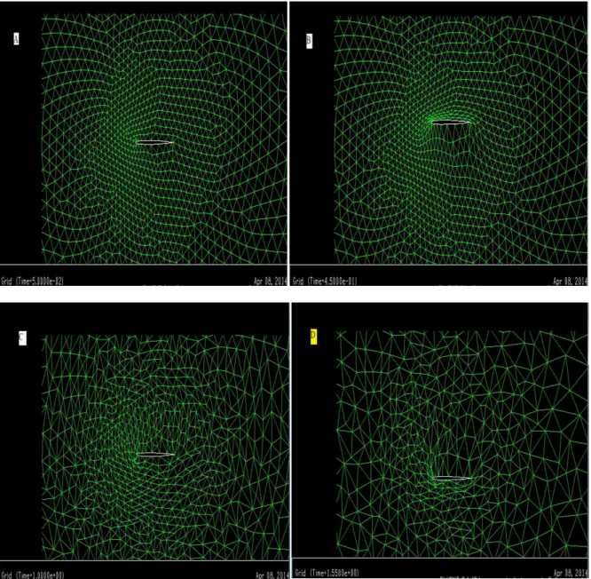
3.4.1 Grid motion

The following figures show the changes that occurs to the initial mesh due to dynamic meshing. It can be seen from the figures that the grid becomes coarser with increase in time.

(19)

14

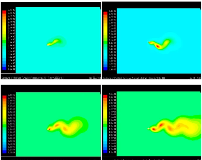
3.4.2 Vortices

The following figures show the inverse Kármán vortex system(visualised using modified turbulence viscosity simulation) in the wake of a NACA0012 aerofoil undergoing pure heaving motion. Massive leading edge vortex shedding is quite clearly visible in the pictures.

Figure 2: Modified turbulence viscosity contours

3.4.3 Velocity profile

As described in the section on The Physics of Drag and Thrust Generation Due to aerofoil Flapping a thrust producing vortex system produces a jet like velocity profile in the wake and a drag producing vortex system produces the opposite.

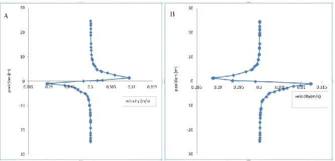
The following (A and B ) velocity profiles are the results of a simulation done on NACA0012 aerofoil(cord length 1m) at a Reynolds number of 20000, reduced frequency of 0.75 and plunge amplitude of 0.4m. With these parameter the aerofoil produces only drag. Reduced frequency is a non dimensional number. It is a parameter that defines the degree of unsteadiness.

(20)

15

Reduced frequency = , where f is the frequency of oscillation and c is the cord

Position in the graphs are the positions on a line perpendicular to the cord line at a distance of 4m from the leading edge.

Figure : A is the velocity profile at a time t < T/2 and B is the velocity profile at a time t>T/2, where T is the time period of the plunging (T = 27.9 s).

The following velocity profile is the result of a simulation done on NACA0012 aerofoil(cord length 1m) at a Reynolds number of 20000, reduced frequency of 5 and plunge amplitude of 0.4m. With these parameter the aerofoil produces thrust.

(21)

16

3.4.4 Variation in coefficient of thrust

In this section results of two sets simulations done on a pure plunging NACA 0012 aerofoil are presented. In the first set of simulations, the variation of the coefficient of thrust when the reduced frequency was kept constant while the plunge amplitude was varied was studied. In the following figure the coefficient of thrust is plotted as a function of the product of reduced frequency and plunge amplitude. It can be seen that the coefficient of thrust continues to increase with increasing kh values despite the fact that strong leading-edge vortices are shed by the aerofoil. However the massive leading-edge vortex shedding causes great reduction in the value of coefficient of thrust for a given value of kh at low k.

Figure : Coefficient of thrust as a function of kh for constant k.

In the second set of simulations, we study the variation of the coefficient of thrust when the plunge amplitude was kept constant while the reduced frequency varied. In the following figures the coefficient of thrust is plotted as a function of the product of reduced frequency and plunge amplitude and also as a function of reduced frequency .

Figure : Mean thrust coefficient generated by pure plunging at various amplitudes and frequencies.

(22)

17

3.5 Pure Pitching

In this section results of the simulations done on a NACA0012 aerofoil undergoing pure pitching motion are presented. The vortex system that is produced due to pure plunging is shown. The velocity profile behind the aerofoil for two different cases and the variation in the coefficient of thrust with different parameters are shown in subsequent sections.

3.5.1 Vortices

The following figures show the inverse Kármán vortex system(visualised using modified turbulence viscosity simulation) in the wake of a NACA0012 aerofoil undergoing pure pitching motion.

Figure 2: Modified turbulence viscosity contours

3.5.2 Velocity profile

(23)

18

The following velocity profile is the results of a simulation done on NACA0012 aerofoil(cord length 1m) at a Reynolds number of 20000, reduced frequency of 1 and pitch amplitude of 15 degrees. With these parameter the aerofoil produces only drag. Position in the graphs are the positions on a line perpendicular to the cord line at a distance of 4m from the leading edge.

Figure : Negative jet like velocity profile of a drag producing wake

The following velocity profile is the result of a simulation done on NACA0012 aerofoil(cord length 1m) at a Reynolds number of 20000, reduced frequency of 7 and pitch amplitude of 15 degrees. With these parameter the aerofoil produces thrust.

Figure : Jet like velocity profile of a thrust producing wake

3.5.3 Variation in coefficient of thrust

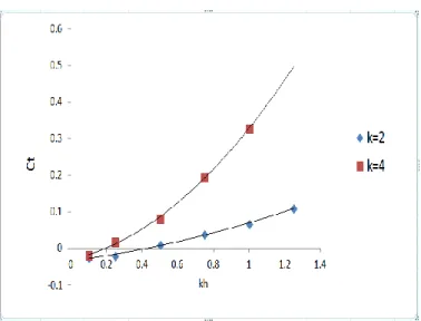
In this section results of three sets simulations done on a pure pitching NACA 0012 aerofoil are presented. In each of these sets of simulations, we consider the variation of the coefficient of thrust when the pitch amplitude was kept constant while the reduced frequency was varied.

(24)

19

The simulations where done for pitch amplitudes of 2, 4 and 15 degrees. The results are shown in the following figure. It can be seen that for a given value of k (greater than 5) the coefficient of thrust increases with the increase in value of pitch amplitude. At lower values of k the aerofoil produces strong von Karmen vortex sheet which is reason for higher drag for higher value of pitch amplitude.

Figure : Mean thrust coefficient generated by pure pitching at various amplitudes and frequencies.

3.6 Combined Pitching and Plunging

In this section results of the simulations done on a NACA0012 aerofoil undergoing Combined Pitching and Plunging motion are presented. The Velocity Magnitude Contours that is produced due to Combined Pitching and Plunging is shown. The velocity profile behind the aerofoil for two different cases and the variation in the coefficient of thrust with different parameters are shown in subsequent sections.

(25)

20

3.6.1 Velocity Magnitude Contours

The following figures show the Velocity Magnitude Contours of a NACA0012 aerofoil undergoing Combined Pitching and Plunging motion. The phase difference is zero for this simulation.

Figure 2: Velocity Magnitude Contours contours

3.6.2 Velocity profiles

The following velocity profile is the result of a simulation done on NACA0012 aerofoil(cord length 1m) at a Reynolds number of 20000, reduced frequency of 1.5, plunge amplitude of 0.4m, pitch amplitude of 4 degrees and phase difference of 0 degrees. With these parameter

(26)

21

the aerofoil produces only drag. Position in the graphs are the positions on a line perpendicular to the cord line at a distance of 4m from the leading edge.

Figure : Negative jet like velocity profile of a drag producing wake

The following velocity profile is the result of a simulation done on NACA0012 aerofoil(cord length 1m) at a Reynolds number of 20000, reduced frequency of 1.5, plunge amplitude of 0.4m, pitch amplitude of 4 degrees and phase difference of 180 degrees.

(27)

22

3.6.3 Variation in coefficient of thrust

In this section results of two sets simulations done on a flapping NACA 0012 aerofoil are presented. In each of these sets of simulations, we examine the variation of the coefficient of thrust when the pitch amplitude, plunge amplitude, and phase difference was kept constant while the reduced frequency was varied. The simulations where done for pitch amplitudes of 4 degrees, plunge amplitude of 0.4m and for two phase differences of 0 and 180 degrees. The results are shown in the following figure. It can clearly be seen that for phase difference of 0 degrees, the aerofoil produces only drag, which keeps increasing with increasing k. In the contrary for the phase difference of 180 degrees the aerofoil produces thrust, which also keeps increasing with increasing k. It is very clear from the results that the phase difference is a crucial variable in flapping motion.

Figure : Mean thrust coefficient generated by pure pitching at various amplitudes and frequencies.

(28)

23

3.7 Conclusion

• For a given value of reduced frequency, it was found that pure plunging generated more thrust than pure pitching.

• Pure pitching motion requires the aerofoil to be oscillated at very high frequency to produce thrust.

• For a given value of pitch and plunge amplitude, it was found that the value of phase angle has a great influence on the thrust generation.

• Combined pitching and plunging motion is the most effective way of producing thrust in the three motions considered.

• It was found that the trends got in the numerical solutions for the variation of

coefficient of thrust were qualitatively correct when compared to experimental results [1][2].

There were variation in the values when compared quantitatively to experimental results, this mainly because of the following :

• The mesh used for the analysis was very coarse.

• The time step used during the simulation were on the higher side. • The convergence limit was set at 0.001.

(29)

24

Reference

(1) Tuncer, I. H., Walz, R., and Platzer, M. F., “A Computational Study of the Dynamic Stall of a Flapping Airfoil,” AIAA Paper 98-2519, June 1998.

(2) Young, J., and Lai, J. C. S., “Oscillation Frequency and Amplitude Effects on the Wake of a Plunging Airfoil,” AIAA Journal, Vol. 42, No. 10, 2004, pp. 2042–2052.

(3) Taylor, G. K., Nudds, R. L., and Thomas, A. L. R., “Flying and Swimming Animals Cruise at a Strouhal Number Tuned for High Power Efficiency,” Nature (London), Vol. 425, Oct. 2003, pp. 707–711. doi:10.1038/nature02000

(4) Garrick, I. E., “Propulsion of a Flapping and Oscillating Airfoil,” NACA, Rept. 567, 1936.

(5) Max F. Platzer, et el, “Flapping-Wing Aerodynamics: Progress and Challenges,” AIAA JOURNAL , Vol. 46, No. 9, September 2008

(6) J., D., DeLaurier, “An Aerodynamic Model For Flapping Wing Flight”, Institute of Aerospace Studies, University of Toronto, Downsview, Ontario, Canada

(7) Katzmayr, R., “Effect of Periodic Changes of Angle of Attack on Behavior of Airfoils,” NACA TM 147, Oct. 1922

(8) von Kármán, T., and Burgers, J. M., “General Aerodynamic Theory Perfect Fluids,” Aerodynamic Theory, edited by W. F. Durand, Vol. 2, Julius Springer, Berlin, 1934, p. 308. (9) Theodorsen, T., “General Theory of Aerodynamic Instability and the Mechanism of Flutter,” NACA, Rept. 496, 1935.

(10) Jones, K. D., Lund, T. C., and Platzer, M. F., “Experimental and Computational Investigation of Flapping Wing Propulsion for Micro Air Vehicles,” Fixed and Flapping Wing Aerodynamics for Micro Air Vehicles, Vol. 195, Progress in Astronautics and Aeronautics, AIAA, New York, 2001, pp. 307–339, Chap. 16.

(11) Lai, J. C. S., and Platzer, M. F., “Jet Characteristics of a Plunging Airfoil,” AIAA Journal, Vol. 37, No. 12, 1999, pp. 1529–1537.

(12) Heathcote, S., Wang, Z., and Gursul, I., “Effect of Spanwise Flexibility on Flapping Wing Propulsion,” Journal of Fluids and Structures, Vol. 24, No. 2, 2008, pp. 183–199. (13) Knoller, R., “Die Gesetze des Luftwiderstandes,” Flug- und Motortechnik (Wien), Vol. 3, No. 21, 1909, pp. 1–7.

(14) Betz, A., “Ein Beitrag zur Erklaerung des Segelfluges,” Zeitschrift fur Flugtechnik und Motorluftschiffahrt, Vol. 3, 1912, pp. 269–272.

(30)

25

Appendix A

User Defined Functions (udf)

(1) The following is the udf used for pure plunging motion of reduced frequency of 2 and plunge amplitude of 1.25 m :

#include "udf.h"

DEFINE_CG_MOTION(piston,dt,vel,omega,time,dtime)

{ vel[1]=0.375*cos(0.6*time);

}

(2) The following is the udf used for pure pitching motion of reduced frequency of 3 and pitch amplitude of 15 degrees :

#include "udf.h"

DEFINE_CG_MOTION(piston,dt,vel,omega,time,dtime)

{ omega[2]=-0.2355*cos(0.9*time);

}

(3) The following is the udf used for combined pitching and plunging motion of reduced frequency of 3, pitch amplitude of 4 degrees, plunge amplitude of 0.4 m and phase difference of 180 degrees : #include "udf.h" DEFINE_CG_MOTION(piston,dt,vel,omega,time,dtime) { vel[1]=0.36*cos(0.9*time); omega[2]=0.0628*cos(0.9*time); }

Aerodynamics of Bird Flight