Non-linear vibrations of tensegrity structures

Non-linear vibrations of tensegrity structures

A thesis submitted to KTH Mechanics

in Royal institute of technology

to fulfill the requirements

for a degree of

Master of Science in Engineering Mechanics

by

Hooman Ahmadian Saieni

ii

List of Contents

2.5. Tangent stiffness matrix ... 6

2.6. Mass matrix ... 7

Chapter3: Direct time integration method ... 11

3.1. Definition ... 11

3.2. Explicit methods ... 13

3.2.1. Central difference method ... 13

3.3. Implicit methods ... 16

3.3.1. Newmark family of methods ... 16

3.3.1.1. Newmark’s method for linear problems ... 17

3.3.1.2. Newmark’s method for non-linear problem ... 19

3.3.1.3. Stability of Newmark’s method ... 22

3.4. Selection of direct integration method ... 22

Chapter4: Problems of study ... 24

4.1. Problem with one degree of freedom ... 24

4.1.1. Linear mass-spring problem ... 24

4.1.1.1. Linear mass-spring system to solve with central difference method ... 24

4.1.1.2. Linear mass-spring system to solve with Newmark’s method ... 24

iii

4.2.1. Elastic pendulum ... 25

4.2.1.1. Elastic spring pendulum ... 25

4.2.1.2. Elastic bar pendulum ... 26

4.2.2. Problem of bar- spring ... 27

4.2.2.1. Problem of low stiff bar- spring ... 27

4.2.2.2. Problem of stiff bar- spring ... 29

4.2.3. Problem of cable-bar ... 29

4.2.3.1. Problem of cable-bar with slackening... 29

4.2.3.2. Problem of cable-bar with slackening and snapping ... 30

4.3. Problem with multi degrees of freedom ... 31

4.3.1. Problem of x-frame tensegrity ... 31

4.3.1.1. Problem of x-frame tensegrity without snapping ... 31

4.3.1.2. Problem of x-frame tensegrity with snapping ... 32

Chapter 5: Results... 33

5.1. Results of one degree of freedom problems ... 33

5.1.1. Results of first spring-mass problem ... 33

5.1.1.1. Solution with central difference method ... 33

5.1.1.2. Solution with exact method ... 33

5.1.2. Results of second spring-mass problem ... 35

5.1.2.1. Solution with Newmark’s method ... 35

5.1.2.2. Solution with exact method ... 36

5.2. Results of two degrees of freedom problems ... 37

5.2.1. Results of pendulum problems... 37

5.2.1.1. Results of spring pendulum problem ... 37

Solution with Newmark’s method ... 37

Verification of results ... 40

Solution with central difference method ... 42

5.2.1.2. Results of bar pendulum problem ... 45

Solution with Newmark’s method ... 45

iv

Solution with central difference method ... 48

5.2.2. Results of bar-spring problems ... 48

5.2.2.1. Results of low stiff bar-spring ... 48

Solution with Newmark’s method ... 48

Solution with central difference method ... 50

5.2.2.2. Results of stiff bar-spring (cable) ... 52

Solution with Newmark’s method ... 52

Verification of results ... 55

5.2.3. Problem of cable-bar ... 57

5.2.3.1. Problem of cable-bar with slackening... 57

Solution with Newmark’s method ... 57

Solution with central difference method ... 59

5.2.3.2. Problem of cable-bar with slackening and snapping ... 59

Solution with Newmark’s method ... 59

5.3. Results of multi degrees of freedom problems ... 61

5.3.1. Results of X-frame tensegrity ... 61

5.3.1.1. X-frame without slackening ... 61

Solution with central difference method ... 61

Solution with Newmark’s method ... 63

5.3.1.2. X-frame with slackening ... 64

Solution with central difference method ... 64

Solution with Newmark’s method ... 67

Chapter 6: Discussion ... 68

Chapter 7: Conclusion ... 70

v

Abstract

A study has been done on different methods to solve the linear and non-linear problems with single or multi degrees of freedom structures. To do that direct time integration methods are used to solve the dynamic equilibrium equations. It has been tried to perform general methods to apply in most structures. In this thesis structures are made of cables and bars but the solution methods which is presented can be applied for any structure, and to utilize those implicit and explicit methods for all structures it is needed to know the tangent stiffness matrix and mass matrix for the structure. Then, it would be possible to analyze the dynamic response of structures under general loads and by general it can be understood that by application of arbitrary forces on different nodes of structure, the method generates result based on applied forces. It is crucial to get the right tangent stiffness matrix and mass matrix to know the dynamic equation in each node. Hence, the method will then work correctly to solve the dynamic problems. More, a parametric study has been done to see the effects of times step, stiffness of elements, length of elements, and other mechanical properties of elements, and this parametric study enables one to produce new results by changing every parameter. Also, continuation of the study on x-frame tensegrity has been done by solving them to check out dynamic response of structure with proposed methods of this thesis. Moreover, a method is presented to use the codes of solver methods of current thesis to apply them for other structures. Hence, as a future work, one can combine the codes of structures and solver codes of this thesis for dynamic response of structure. In fact the main effort of this thesis is on presenting different methods to solve various structures.

1

Chapter 1: Introduction

1.1. Background

Dynamic response of structures is interesting for structural engineers and has high importance among earthquake engineers. Actually, the present study is continuation of response of structure in dynamics. First, a structure is presented, and that would be any kind of structure, one can indicate a structure like tensegrity that is the main structure in this thesis, but that can be any kind of structure to consider it for earthquake response. Since the subject of this project is non-linear vibration of tensegrity structures, the word of earthquake suits the meaning of whole project for a structure like tensegrity. Tensegrities are structures made of cables and bars which have specific usages like creating sculptures, domes and so on. In addition, tensegrity structures has low stiffness but studying this kind of structures enables one to calculate more complex structures in future because the procedure of calculations are the same just the elements of structures can change like changing bar to beam and so on. Apart from low stiffness of tensegrity structures, there are some topics like slackening of cables in structure which can be important and that must be taken into account.

The reason for choosing a tensegrity structure is the experiences in this topic at the Department of Mechanics of Royal institute of Technology. As a result, a study on different methods of solving non-linear problems has been done to meet the expectations of this project.

To solve the dynamics of tensegrity structures, direct time integration methods were used. Implicit and explicit method like Newmark’s method and central difference method are performed as most well know methods of direct time integration methods to solve tensegrity structures. Direct time integration methods have been used widely to capture dynamic response of structures. Most recently, Irfan Baig and Grätsch (2009) took a survey on recommendations for practical use of numerical methods for linear and non-linear dynamics but most of their research was on single degree of freedom systems. So, this thesis is a continuation their research on multi degrees of freedom systems to solve with numerical methods.

Moreover, for tensegrity structures, to solve with direct time integration methods, it is important whether they are prestressed or not. For structure to be stable they should be prestressed and in both cases they can be analyzed with direct time integration methods. However, for obtaining stiffness of prestressed frameworks, Guest (2006) has presented a unifying approach to get the stiffness matrix of tensegrity structure. Furthermore, to prestress a tensegrity structure, Pellegrino and Calladine (1985) introduced a matrix analysis of

2

indeterminate frameworks, then Pellegrino (1993) presented SVD1 method to analyze equilibrium matrix of tensegrity structure. Most importantly, Géradin and Rixen (1994) published a book as Mechanical Vibration which is the main reference of this project as it includes algorithms which are used to solve for the dynamic response of structures. Also, Murakami (2000) has done a research on static and dynamic analysis of tensegrity structures with linearized Lagrangian equations. Furthermore, Tran and Lee (2010) introduced a method for initial self-stress design of tensegrity structure. Moreover, Oliveto and Siavaselvan (2011) performed dynamic analysis of tensegrity structure in the small displacement regime.

In fact, there were many efforts to understand details of tensegrity structures in static and dynamic cases. Most efforts have been on prestressing, form-finding, statical and dynamical analysis of tensegrity structures. In this thesis, it is tried to find an applicable method to solve the tensegrity structures in the dynamic cases. So, the main effort of this thesis is finding a general method to solve the tensegrity structures to find dynamic responses with given external load.

As a matter of fact, by taking previous efforts into account, it can be assumed that a tensegrity structure that could be or not to be prestressed, must be solved for dynamic cases. Then, direct time integration methods will be presented to solve tensegrity structures in dynamic cases.

1.2. Motivation

Capturing the response of tensegrity structures with different modules is the main motivation of this project but as it has been pointed out before if one is successful to analyze the dynamic behavior of tensegrity structure, it will be possible to perform the solution methods to more complex and complicated structures. In that case that is really crucial how to record the tangent stiffness matrix and mass matrix of complex structures.

1.3. Objectives

The objective of this thesis is to develop a numerical procedure for the dynamic analysis of tensegrity structures which are made of cables and trusses which are subjected to random external forces. The equations of motions of structure are derived from standard method of structural dynamics. Moreover, the study has been done to see the effects of time step, stiffness of bars, stiffness of cables, slackening of cables, and initial conditions of structure. Since, that is a parametric study; the effect of each parameter can be captured in the final result of the dynamic analysis of structure.

1

3

1.4. Overview

The solution of tensegrity structures is achieved by usage of implicit or explicit methods for tensegrity structures in dynamic problems. The implicit and explicit methods which have been used in this thesis are written and developed to calculate dynamic responses.

In the second chapter, different points in matter of tensegrity are presented. In the third chapter, direct time integration methods have been introduced. Implicit and explicit methods with details of them are presented in third the chapter. More, in the fourth chapter, the problems of the study are presented. Actually, problems are defined to find out the differences between methods to solve the problems in single or multi degrees of freedom structures. Then, results are presented in fifth chapter. Finally, last two chapters are devoted to discussion and conclusions to find the final outcomes of this project.

4

Chapter 2: Tensegrity

2.1. Definition

There are many studies about concept of tensegrity. Tensegrity structures are spatial structural systems composed of struts and cables with pin-jointed connections, and their stability comes from the self-stress state in their tensioned and compressed members. Tensegrity structures can be used in modern structural engineering. To find a widely acceptable definition for tensegrity, the definition of Motro is more respectable which says: “A tensegrity is a system in stable self-equilibrated state comprising a discontinuous set of compressed components inside a continuum of tensioned components”. [1]

One of the main requirements for a structure to be categorized as a tensegrity structure is that its initial prestressed configuration must be in stable equilibrium in absence of external forces. [2]

2.2. Application

These kinds of structures denoted tensegrity are interesting among architects and engineers. Tensegrity structures in most cases are very light and that is an important property to be used in space. Specially, if the structure inherited the deployability, that would be interesting to be used in space structures.

Furthermore, stiffness of tensegrity structures is not great, and because of not being stiff, they have special usages. More, structural damping is low for this kind of structure, and that would lead to increase sensitivity with dynamic loading.

The stability of tensegrity structures should be supported by self-stress of tensions and compressions in elements of structure. Moreover, non-linear behavior which comes from geometry non-linearity is expected when dynamic loading performed on the structure.

2.3. Form-finding

Form-finding is an expression which mostly used when subject is the tensegrity, and it is a procedure of finding self-stress state in whole structure of tensegrity and how to join different elements of structure together.

Also, the procedures of defining forces in each element of structure are called designing of self-stress for initial condition. As it has mentioned before, in tensegrity, cables are used for tensions and bars to take compression forces. [3]

Every structure made of a module or it can be multimodular. The modules of tensegrity can be x-module, T3 module or other types.

5

2.4. Equilibrium matrix

Moreover, to solve the initial self-stress of tensegrity structures, the equilibrium matrix A must be defined. That can be a square matrix but in most cases it is a rectangular matrix and that can be obtained from the equilibrium equation:

Where is generalized stresses and l is the vector of generalized loads. In general, the coefficients of the equilibrium matrix are functions of the geometrical configuration of the assembly. The dimension of this matrix is very important by knowing the number of rows and columns, and can be defined. More, the size of l is but the size of is .

By defining the rank r of the equilibrium matrix, the key parameters which show behavior of structure can be written as:

By deriving the parameters of m and s other properties of structure can be found in Table 2-1. The values of m and s do not have high importance but it is essential to know that those parameters are equal to zero or not.

Then, to solve the formulation of initial self-equilibrium equations that must be noted that external and self-weight of the structure can be neglected. So, to solve the system, singular value decomposition (SVD) of equilibrium matrix is used. By using SVD, the equilibrium matrix will be changed to what can be seen below:

Where U is an orthogonal matrix with dimension of Likewise, W is an orthogonal matrix with dimension of , and V is a matrix with dimension of .

More, to choose the rank of the equilibrium matrix it must be noted that:

6

Type

s=0

m=0

s=0

m>0

s>0

m=0

s>0

m>0

Also, the V matrix has r non-zero elements on the leading diagonal, and the rest of the elements of matrix are zero. Hence, the V matrix contains up to singular values. [5, 6]

To analyze static and dynamic responses of pre-stressed tensegrity structures, it is extremely important to compute infinitesimal mechanisms of tensegrity modules and to interpret global deformation modes of tensegrity structures in terms of infinitesimal mechanisms modes. [7]

2.5. Tangent stiffness matrix

After finding the equilibrium matrix, tangent stiffness of whole structure can be specified as: ̂

Where is the equilibrium matrix for the whole structure, ̂ is a diagonal matrix of modified axial stiffness, and is the stress matrix for the entire structure. The tangent stiffness matrix consist of material stiffness and geometric stiffness which in first one, the structure is maintained in its initial geometry, and second one is about the time when stiffness changed because of reorientation of stressed members. Also, due to increase in axial forces.

It is crucial to know that when external load and self-weight are ignored, the tensegrity does not need any fixed node, and geometry of the tensegrity structure can be defined by position of nodes, and the whole system can be assumed as free-standing, forming a rigid body in space.[8]

7

𝒖_𝟐 𝒖_𝟏

𝑳

2.6. Mass matrix

For a linear bar element shown below

Where the length is L, cross sectional area A, and the density . A linear displacement function is assumed in the X direction as:

The number of coefficients in the displacement function is equal to the number of degrees of freedom associated with the element. Moreover, the displacement function in terms of shape function can be defined as below:

[ ]=, -

The typical method to derive the consistent mass matrix is the principle of virtual work. By substitution of shape functions in the above equation, mass matrix equation gives:

∫ [ ]* + ∫ [ ]* + ∫ [ ]

Then, by evaluating the above integral, consistent mass matrix is computed as follow:

* +

By assuming that the length of bar is and discretizing the bar into two elements with length for each element, lumped mass matrix is defined as below:

* + *

+

𝑳 𝑳

8 Then the global lumped mass matrix is defined as:

[ ]

In general, the result of consistent mass matrix is closer to available analytical and experimental results than those which use the lumped mass matrix. Surprisingly, for bar elements, the results of lumped mass matrix are as good as or even better than the result of those are used consistent mass matrix. However, from the mathematical point of view, consistent mass matrix approach yield an upper bound on the frequencies but for lumped mass matrix approach has no mathematical proof of boundless.

As a general rule, the construction of the structure mass matrix largely parallels that of tangent stiffness matrix . Mass matrices for individual elements are formed in local coordinates then transformed to global, and merged into the tangent mass matrix following exactly the same techniques used for .

An important difference with the stiffness matrix is the possibility of using a diagonal mass matrix based on direct lumping. More, a lumped mass matrix entails significant computational advantages for calculations of [20].

Mass matrix must satisfy special conditions and it can be used for verification and debugging. So, a mass matrix should have properties as follow:

 Matrix symmetry, which means .  Physical symmetry must be reflected in mass matrix.

 Conservation. At a minimum, total element mass must be preserved. This is easily verified by applying a uniform translational velocity and checking that linear momentum is conserved.

 Positivity, which shows must be nonnegative. Also, for any nonzero velocity field defined by the node values ̇ ̇ ̇ .

Also, like the tangent stiffness matrix, mass matrices are developed in a local or element frame, and they must be globalized before assembling to tangent mass matrix. The transformation applied as follow:

̅̅̅̅

Where ̅̅̅̅ is element’s mass matrix, referred to the local frame, and is the local to global displacement transformation matrix, and it is derived from transformation which is used for stiffness globalization. Moreover, for stiffness matrices, is often rectangular if the local

9

stiffness has lower dimensionality. Globalization to and involves application of and transformation matrices.

It is important to know that unlike stiffness, translational masses never vanish. So, translational mass cannot be zero. Conclusion is that all translational masses must be retained in the local mass matrix.

For a two node bar element which has two degrees of freedom each node, the local consistent and lumped mass matrices are shown below:

̅̅̅̅ _{[ ]} ̅̅̅̅ _[ ]

Then by globalizing the local consistent and mass matrices by transformation matrix ̅̅̅̅ the results are ̅̅̅̅ and ̅̅̅̅ . Hence, the mass matrices repeat.

̅̅̅̅ ̅̅̅̅

And for consistent matrix is proved as can be seen below:

̅̅̅̅ _[ ̃ ̃] , [ ] , and ̃ * + , , [ ] [ ̃ ̃] [ ] [ ̃ ̃ ̃ ̃] [ ̃ ̃] ̅̅̅̅

The same conclusion holds for 3D. So, the contents and order of ̃ are irrelevant to the result. Hence, the following generalization follows [20].

10

The repetition rule can be expected to fail in the following scenarios:

 The element has non-translational degrees of freedoms.

 The mass blocks are different in content or size. This occurs if different models are used in different directions. Examples are furnished by beam-column, element with curved sides or faces, and shell elements.

 Nodes are referred to different coordinate frames in the global system. This can happen if certain nodes are referred to special frames to facilitate the application of boundary conditions.

11

Chapter3: Direct time integration method

3.1. Definition

To solve the structural dynamic equations of motion for arbitrary excitation, two methods are useful; modal superposition techniques and direct time-integration methods. The modal superposition technique is based on results from linear modal analysis, and consists of expressing the dynamic response in an eigenmode series expansion, and that is an effective method since the fundamental modes predominate in the response but for a high number of modes, this technique should be replaced by direct integration method.

The most general approach for the solution of the dynamic response of structural systems is the direct numerical integration of the dynamic equilibrium. Direct time integration techniques are not limited to the linear case as they can be easily extended to non-linear systems and this method makes it possible to use for high frequency components. In using direct time integration, the attempt is to satisfy dynamic equilibrium at discrete points in time, and to do that, most methods use equal time steps for each time interval. All methods are classified as implicit or explicit direct integration method.

In general, direct multistep integration methods for first order systems of the form ̇ can be stated as:

∑

∑ ̇

Where is the computational time step, and

*

̇ +

is the state vector which is calculated at time from the state vector at the m preceding times, from their derivatives and from the derivatives of itself.

 leads to an implicit scheme which is a scheme where the evaluation requires the solution of system of equations. Actually, the state vector at time is a function of its own time derivative. So, for the non-linear case the method will be iterative. Actually, an implicit method attempt to satisfy the differential equation at time t from the solution at time .

This method requires the solution of a set of linear equation at each time step, and larger time steps can be used.

12

 corresponds to an explicit scheme which is a scheme where the evaluation of

does not require the solution of any system of equations and instead can be

concluded from the results of previous time steps. In fact, explicit methods use the differential equation at time t to predict solution at time , and very small time steps are needed. An explicit method is conditionally stable with respect to size of time step.

In fact, explicit methods do not involve the solution of linear equations at each step, and these methods use differential equation at time to predict solution at time . In reality for real structures with stiff elements, a very small time step is needed to reach a stable solution. Therefore, all explicit methods are conditionally stable and the stability depends on the chosen time step.

On the other hand, implicit methods struggle to satisfy the differential equation at time when at time the solution is found. Hence, at each time step, implicit methods require solution of a set of linear equations, and larger time steps can be used. Moreover, these methods can be conditionally or unconditionally stable.

There are many accurate, higher orders, multi-step methods for numerical solution of differential equations, which are assuming that higher derivatives are smooth but the second derivative of displacement, which is acceleration, is not a smooth function, and that cause non-linearity of solutions for structures. So, the conclusion is that single-step, implicit, unconditional stable methods can be used to solve practical structures.

For implicit method, an interesting and useful method is the Newmark method that can be called Newmark family of methods, and for the explicit one, an example is Central difference method.

In order to obtain an effective solution of a dynamic response, it is important to choose an appropriate time integration scheme. This choice depends on the finite element idealization, which in turn depends on the actual physical problem to be analyzed. It follows therefore that the selection of an appropriate finite element idealization of a problem and the choice of an effective integration scheme for the response solution are closely related and must be considered together. The finite element model and time integration schemes are chosen differently depending on whether a structural dynamic or a wave propagation problem is solved.

For structural dynamics, the basic consideration in the selection of an appropriate finite element model of a structural dynamics problem is that only the lowest modes of a physical system are being excited by the load vector. There is no need to represent the higher

13

frequencies of the actual physical system accurately in the finite element system because the dynamic response contribution in these frequencies is negligible.

The observation that the use of higher order elements can be effective with implicit time integration in the analysis of structural dynamics problems is consistent with the fact that higher order elements have generally been found to be efficient in static analysis, and structural dynamics problems can be thought of as static problems including inertia effects. If the finite element idealization consists of many elements it can be more efficient to use explicit time integration with a lumped mass matrix in which case no effective matrix is assembled and triangularized but a much smaller time step must generally be used in the solution. [9]

An important observation was that the cost of a direct integration analysis is directly proportional to the number of time steps required for solution. [10]

3.2. Explicit methods

3.2.1. Central difference method

This method is an explicit method, and this method is Newark’s method with and . So, two main equations of Newark’s method change to following equations by assumption of :

̇ ̇ ̈ ̈

̇ ̈

To write an algorithm for Central difference method, half-time interval is calculated as:

Consequently, for a constant time step h, acceleration is calculated as:

̈

14 ̇

̇ ( )

So, acceleration based on half-time is written as:

̈

( ̇

̇ )

The stability domain is such where the highest frequency in the model is . This stability condition named as Courant condition, and is taken as the highest of the eigenfrequencies of the individual elements since it corresponds to an upper bound to the eigenfrequencies of the complete model.

Central difference method is generally much less computationally expensive and becomes almost trivial when the so-called lumped mass finite element formulation is used. The explicit methods are very effective at handling various non-linearities. Moreover, in implicit methods, non-linearity generally causes some residual imbalance between internal and external forces which is iterated to equilibrium because of using iterations in Newton-Raphson procedures. There are some advantages for explicit methods like simplicity and directness but disadvantages for stability and accuracy required very small time step which in implicit the time step can be large in comparison with explicit methods and they are stable. After all, here there are some advantages and disadvantages for explicit methods:

Advantages for explicit methods [21]:  Robustness and efficient

 Useful for more advanced materials  Directness of reaching to answer

Disadvantages:

 Small time step required for calculation  Expensive about computational speed  Solution can diverge

15

In the picture below, flowchart of the central difference method can be seen:

Figure 3-1: Flowchart for central difference method, [9]. INITIAL REQUIRED INFORMATION M,C,K, 𝑭 & 𝒖_𝟎𝒖̇_𝟎 𝒖̈_𝟎 𝑴 𝟏 _𝑭 𝟎 𝑲𝒖𝟎 𝒕𝟏 𝟐 𝟏 𝟐𝒉𝟏 𝒖̇𝟏 𝟐 𝒖̇_𝟎 𝒉𝟏 𝟐 𝒖̈𝟎 𝒕_𝒏 𝒕 𝒏 𝟏_𝟐 𝟏 𝟐𝒉𝒏 TIME INCREMENT 𝒖_𝒏 𝒖_{𝒏 𝟏} 𝒉_𝒏𝒖̇ 𝒏 𝟏_𝟐 DISPLACEMENT INCREMENT 𝒕 𝒏 𝟏_𝟐 𝒕𝒏 𝟏 𝟐𝒉𝒏 𝟏 SECOND TIME INCREMENT

𝒖̈_𝒏 𝑴 𝟏 𝑭_𝒏 𝑲𝒖_𝒏 ACCELERATION COMPUTATION 𝒖̇ 𝒏 𝟏_𝟐 𝒖̇𝒏 𝟏_𝟐 𝒉𝒏 𝟏_𝟐𝒖̈𝒏 VELOCITY INCREMENT

16

For single degree of freedom systems the central difference method is most accurate, and the linear acceleration method is more accurate than the average acceleration. If only single degree of freedom systems are to be integrated there is no need to use an approximated method. It appears that the modified average acceleration method with addition of minimum proportional damping is a general procedure that can be used for dynamic analyses of all structural systems. For earthquake analysis of linear structures, it should be noted that the direct integration of the dynamic equilibrium equations is normally not numerically efficient in comparison with superposition method using LDR vectors. [22]

The advantage of using Newmark’s method over the central difference method are that Newmark’s method can be made unconditionally stable if and . Also, larger time steps can be used, and the results will be better and more accurate.

From the computational point of view, central difference method can be computationally more efficient but to get more accuracy it is recommended to use accurate explicit methods like Runge-Kutta method which is approximating the slope of the secant of the solution, from one time step to the next one. However the Runge-Kutta method can be four times more expensive than central difference method for a given time step.

However, for multi degrees of freedom systems the central difference method will not be the method of choice. Besides, for multi degrees of freedom systems, the choice of a time integration scheme depends on the nature of the problem. In cases which most part of the solution lies on lower modes, the Newmark method is generally preferred, because larger time step can be used. Unlikely, for problems like crash analysis which the solution lies on higher modes, explicit methods are useful. [23]

3.3. Implicit methods

3.3.1. Newmark family of methods

The Newmark method is a single-step direct integration method. In 1959 Newmark presented a family of single-step direct integration method to solve structural dynamic problems. It was originally introduced for solution of second order differential equation arising from dynamic equilibrium in structural dynamics. In past 53 years, the method has been applied to dynamic problems to solve many practical engineering structures, and it has been modified and

17

improved by many researchers. However, the versatility of Newmark’s method is evidenced by its adaptation in many commercial available computer programs.

Newmark method is by far the most popular tool for direct integration of deterministic dynamical systems. [11]

To illustrate the use of Newark’s method consider the solution of the linear dynamic equilibrium equations as:

̈ ̇

For linear system [ ] [ ] and [ ] are independent of time and therefore remain unchanged during the integration procedure.

The direct use of Taylor’s series provides a rigorous approach like this:

̇ ̈

̇ ̇ ̈ ⃛

Newmark truncated equations like this:

̇

̈ ⃛

̇ ̇ ̈ ⃛ By assumption of linear acceleration within the time step ⃛ is:

⃛ ̈ ̈ Finally, standard form of Newmark’s equation becomes:

̇ ( ) ̈ ̈

̇ ̇ ̈ ̈

So, for each DOF (Degree Of Freedom) of structural systems, the Newmark’s method is required iteratively. [9, 12, 13]

3.3.1.1. Newmark’s method for linear problems

18

[ ]

In the flowchart below the Newmark method is introduced for linear systems:

Figure 3-2: Flowchart of Newmark’s method for linear cases [9].

The traditional Newmark family might exhibit deficiencies in the energy conservation and hence numerical stability when it is applied to non-linear transient problems. [14]

INITIAL REQUIRED INFORMATION M,C,K, 𝑭 & 𝒖_𝟎 𝒖̇_𝟎 𝒖̈_𝟎 𝑴 𝟏 𝑭_𝟎 𝑪𝒖̇_𝟎 𝑲𝒖_𝟎 𝑡_𝑛 𝑡_𝑛 𝑡 𝒖̇_𝑛 ∗ 𝒖̇_𝑛 𝛾 𝑡𝒖̈_𝑛 𝒖_𝑛 ∗ 𝒖_𝑛 𝑡𝒖̇_𝑛 ( 𝛽) 𝑡 𝒖̈_𝑛 PREDICTION 𝑺 𝑴 𝛾 𝑡𝑪 𝛽 𝑡 𝑲 𝑺𝒖̈_𝑛 𝑭_𝑛 𝑪𝒖̇_𝑛 ∗ 𝑲𝒖_𝑛 ∗ COMPUTING ACCELERATION ENERGY EVALUATION (OPTIONAL) 𝒖̇_𝑛 𝒖̇_𝑛 ∗ 𝑡𝛾𝒖̈_𝑛 CORRECTION 𝒖𝑛 𝒖𝑛 ∗ 𝑡 𝛽𝒖̈𝑛

19

3.3.1.2. Newmark’s method for non-linear problem

For the solution of non-linear equation of motion, direct numerical integration methods are generally recommended. The basic Newmark constant acceleration method can be extended to non-linear dynamic analysis which requires that iteration should be performed at each time step in order to satisfy equilibrium. Furthermore, the incremental stiffness matrix should be performed and triangularized at each iteration or selective points in time. To minimize the computational requirements, various kind of numerical tricks, including element by element methods, have been developed. Moreover, in some cases, the triangularization of the effective incremental stiffness matrix can be avoided by introduction of iterative solution method. In fact, many non-linear problems admit solutions by linear techniques by enlarging the domain of the problem. [17] In this section, the solution of the non-linear dynamic equations will be discussed without details of actual nature of non-linearities that can be geometric, material or other. So, the equation of motion in non-linear case can be defined as follow by assumption that and ̇ are given:

̈ ̇

The assumption is that the inertia coefficients do not depend on the configuration, and actually it means that the reference state is fixed and the motion is in Cartesian coordinates. Then, to start with implicit method in non-linear cases, the residual vector should be identified as r and can be written as follow:

̈ ̇

Where equations of Newmark’s method can be rewritten as follow:

̈ ∗ ̇ ̇ ∗ ̈ ∗

Then predictors are defined below:

20

̇ ∗ ̇ ̈

∗ _{̇ ( ) ̈}

Residual vector is represented in terms of as .

The iteration matrix is written by:

is the tangent stiffness matrix, is tangent damping matrix, and is mass matrix. The non-linear system is solved by Newton-Raphson iteration method. Correction in time step k of time step n+1 is calculated by solving the linearized equation

( )

Also the corrections for acceleration and velocity is calculated as follow

̈

̇

The Newmark constant acceleration method, with the addition of very small amount of stiffness proportional damping, is recommended for dynamic analysis of non-linear structural systems. It should be noted that in all direct integration methods, it is important to make sure that the stiffness proportional damping does not eliminate important high-frequency response. However, when problem is a non-linear one, one cannot prove that any one method will always converge, and the amount of error in conservation of energy for every solution must be checked. More, that is a predictor-corrector method which the method predict then if it did not converge, the method would correct the prediction. [9]

21

Figure 3-3: Flowchart of Newmark’s method for non-linear cases [9]

To explain the above algorithm, it should be noted that for each time step, iteration start from a perdition of displacement, velocity and acceleration which is zero. The reason to choose prediction of acceleration as zero is fairly stable iteration procedure, and to reach

INITIAL REQUIRED INFORMATION M,C,K, 𝑭 & 𝒖_𝟎 𝒖̇_𝟎 𝒖̈_𝟎 𝑴 𝟏 𝒈_𝟎 𝒇 𝒖̇_𝟎 𝒖_𝟎 𝑡_𝑛 𝑡_𝑛 𝒖̇_𝑛 𝒖̇_𝑛 𝛾 𝒖̈_𝑛 𝒖𝑛 𝒖𝑛 𝒖̇𝑛 𝛽 𝒖̈𝑛 𝒖̈_𝑛 𝟎 PREDICTION 𝒓_𝑛 𝑴𝒖̈_𝑛 𝒇_𝑛 𝒈_𝑛 CALCULATION OF RESIDUAL VECTOR 𝒓_𝑛 𝜖 𝒇 CONVERGENCE? 𝑺 𝒖_𝑛 𝒖 𝒓_𝑛 CORRECTION CALCULATION 𝒖_𝑛 𝒖_𝑛 𝒖 𝒖̇_𝑛 𝒖̇_𝑛 𝛾 𝛽 𝒖 𝒖̈_𝑛 𝒖̈_𝑛 𝛽 𝒖 CORRECTION YES NO

22

convergence the Newton-Raphson is used. Moreover, for each time step, if the prediction was not correct, Newton-Raphson iteration would occur to reach the convergence. So, in the non-linear case, the time step drives the accuracy of integration, and plays the main role in stability of iteration process. Hence, the size of time step is a crucial issue.

3.3.1.3. Stability of Newmark’s method

For zero damping this method is conditionally stable if: , and

√

And is the maximum frequency in structure of system, and this method is unconditionally stable if:

When is larger than errors are introduced. These errors are associated with numerical damping and period elongation.

Also, for big structures with many degrees of freedom, the time step can be written as below:

√

In real structures, computer models normally contain a large number of periods that are smaller than the integration time step. So, it is better to select a numerical integration method that is unconditional for all time steps. is the minimum time period of structure. [22]

The accuracy of the numerical response can be estimated by evaluating the variation of the energies. [19]

3.4. Selection of direct integration method

There are many different direct numerical integration methods, and the difference is using different integration parameters. Some of them can be seen in Table 3-1:

23

Method Amplitude error Accuracy

Central difference 0 0

Excellent for small

Unstable for large

Linear acceleration 0

Very good for small

Unstable for large

Average acceleration 0

Good for small

No energy dissipation Fox & Godwin 0 --- ---

Table 3-1: Summary of direct time integration methods

The Fox & Godwin algorithm leads to a periodicity error of the third order, but is conditionally stable, and the average constant acceleration algorithm is the best unconditionally stable method.

In Newmark family of methods, the average acceleration method is the most robust method since it is unconditionally stable, and it can be used for step by step dynamic analysis of large complex structural systems which has many degrees of freedom and large number of high frequencies and short periods. Also, the average acceleration method can be used to solve linear and non-linear problems. More, calculation of tangent stiffness matrix and forces from displacements at each time step can be quite complicated for non-linear multi degrees of freedom systems. However, there is a problem in performing average acceleration method, and the problem is short periods which are smaller than the time step, oscillate indefinitely after they are excited, and the oscillation in higher modes can be reduced by addition of stiffness proportional damping.[15]

The choice of method for time-history analysis is strongly problem-dependent. The efficiency of a given method depends on whether the problem is of a wave propagation or a structural dynamics type, the time span for which analysis is required, whether response is linear or non-linear, and the topology of the finite element mesh. General speaking, direct integration methods are preferably for non-linear problems. [13]

24

Chapter4: Problems of study

4.1. Problem with one degree of freedom

4.1.1. Linear mass-spring problem

4.1.1.1. Linear mass-spring system to solve with central difference method

This problem is a single degree of freedom, spring- mass system. To start, in the figure below a spring mass system is shown with the one dimensional spring mass.

Figure 4-1: SDOF problem of spring-mass system to solve with central difference method

[ ]

To solve this problem, first the Central difference method is used. Note that and after the time of the becomes zero. As it was mentioned in the part of introducing central difference method in 3.2.1, and ̇ must be known, and both of them are zero in the current example. So, by implementing the central difference method for the current single degree of freedom problem, it can be solved to get displacement, velocity, and acceleration of the system.

To see the result, a graph has plotted in 5.1.1.1 and 5.1.1.2 in 5s to check out how the displacement, velocity, and acceleration of the system are changed.

4.1.1.2. Linear mass-spring system to solve with Newmark’s method

This problem is the same as previous problem but the parameters of mass, stiffness and force has changed as you see in Figure 4-2:

K=100 lb/in

𝐹 𝑡 𝑀𝑎𝑠𝑠

25

Figure 4-2: SDOF problem of spring-mass system to solve with Newmark’s method

[ ] [ ]

After 2 seconds the is zero. Like, the previous problem and ̇ are zero, and .

4.2. Problem with two degrees of freedom

4.2.1. Elastic pendulum

4.2.1.1. Elastic spring pendulum

In this section a spring pendulum will be discussed which is fixed on one of its nodes. The problem is defined as it can be seen in the figure below.

Figure 4-3: Elastic spring pendulum system

It has two degrees of freedom with an absolute coordinates (x,y). Moreover, is the initial length of the pendulum, and √ . By writing the equations of motion, two equations are obtained as follow:

K=70 lb/in 𝐹 𝑡 𝑀𝑎𝑠𝑠 L y x mg K

26

̈

̈

These equations are non-linear equations because of the length expression. Also, tangent stiffness matrix is given as below:

[

_]

Additionally, some other parameters are given like , , , , , , , , and ̇ ̇ . By writing down the equations of motion in matrix form, stiffness matrix can be found as follow: * + [ ̈ ̈] [ ] * + * +

This problem is solved with two methods of central difference method and Newmark’s method and they can be seen in the chapter of results.

4.2.1.2. Elastic bar pendulum

In this section, to show that the codes of implicit and explicit methods are versatile codes, the previous problem is redesigned by changing a stiff bar instead of loose spring. In point of fact, a stiff bar is used to check out that the code works for linear problems or not. This problem is solved with both central difference and Newmark’s method in 5.2.1.2. In figure below, elastic bar pendulum is shown.

27

Figure 4-4: The elastic bar pendulum system

The only difference of current problem with previous one is that stiffness of spring (k ) changed with stiffness of bar which is . So, the dynamic equations can be seen below:

̈

̈

Moreover, the initial conditions are defined as follow: , , and ̇ ̇ . All the rest of parameters are the same as parameters in problem 4.2.1.1 just k is changed to except h which is time step. By choosing E=204 and A=19.6 , the problem is solved. In this case EA/L is much higher than stiffness of spring that was k=30 N/m in previous problem. To understand the differences, in current problem the spring stiffness of bar is about 4 but in last problem the stiffness of spring was just 30 . Hence, the differences are so crystal clear and linear behavior is expected.

4.2.2. Problem of bar- spring

4.2.2.1. Problem of low stiff bar- spring

There is a bar and spring in this problem. Initial length of bar and spring are given. To solve the current problem, equations of motions should be calculated. Then by writing the equations of motions in matrix form, the stiffness matrix can be found. There are two methods to solve this problem, implicit and explicit method. However, explicit methods are

L y

x

mg K

28

faster than implicit method. However, implicit methods are more accurate than explicit methods. The geometry of the problem is defined in the figure below.

Figure 4-5: The elastic spring-bar system

Dynamic equations of system can be written as below.

̈

̈

Above equations can be written in matrix form as follow:

* + [ ̈ _̈] [ ] * ₊ [ ]

Stiffness matrix can be obtained from above equation:

[

]

Also √ , and √ . Furthermore, initial displacement and velocity of current two degrees of freedom are given. Initial conditions can be defined as , , , , , _,

Mass 𝑶𝟏 𝑶𝟐

x y

29 _{, ,}

√ ⁄ , and ̇ ̇ . Results are available in 5.2.2.1.

4.2.2.2. Problem of stiff bar- spring

In this part, problem of 4.2.2.1 is solved but two differences applied. First, stiffness of bar increased dramatically ( ). Secondly, stiffness of spring increased and instead of spring stiffness, EA/L has used which is stiffness of cable ( ). In the current problem, mass is 100kg. In fact, stiff spring is assumed to behave like a cable. Equations of motion are available in 4.2.3.1. It must be noted that just stiffness of spring (k) has changed with stiffness of cable (EA/L). In fact one can call this system a stiff bar-cable. However, in comparison with problem of 4.2.2.1, three items have changed as follow: stiffness of bar changed, stiffness of spring has changed, and instead of k for stiffness of spring, EA/L is used. In fact both elements are bar elements but because of low stiffness of an element in comparison with another one, we called them bar-spring system.

4.2.3. Problem of cable-bar

4.2.3.1. Problem of cable-bar with slackening

This problem is like problems of spring-bar but instead of using a spring, a cable has used. The EA of cable has been chosen to be one tenth of the bar’s EA, and the mass is 115kg. Then, the geometry of this problem is presented below:

Figure 4-6: The elastic cable-bar system

Mass

𝑶_𝟏 𝑶_𝟐

x y

30

Dynamic equations can be written like below equations.

̈ ̈

It is important to know that stiffness of spring (k) in problem 4.2.2.1, has changed to

⁄ . There is a difference between how spring and cable are performing in problems. As the natural behavior of cable, a slackening condition must be added to the problem, and that can be seen below:

if Lcable<L0cable EAcable=0;

else

EAcable=real EA of cable;

end

Additionally, the initial conditions are: m=115kg, , _√ ⁄ , , and ̇ ̇ . Results are available in 5.2.3.1.

4.2.3.2. Problem of cable-bar with slackening and snapping

This problem is like the problem of 4.2.3.1 but the cable snaps after specific elongation. Then, after snapping, stiffness of cable becomes zero. Also, initial conditions are defined as: m=115kg, , , , and ̇ ⁄ , ̇ . More, it can be defined that length of cable changes to zero after slackening (braking or tearing down). These conditions are added to the code of last problem.

if Ls<L0s EAcable=0; else if Ls<Lsnapping EAcable=10000; else if Ls>=Lsnapping EAcable=0; Ls=0; end end

31

To solve the problem it is needed to put above conditions after Newton-Raphson iteration for each time step .The effect of snapping and slackening of the cable can be seen in 5.2.3.2.

4.3. Problem with multi degrees of freedom

4.3.1. Problem of x-frame tensegrity

4.3.1.1. Problem of x-frame tensegrity without snapping

By putting three modules of x-frame tensegrity [16] on top of each other a structure can be made. To start the analysis there are some point that should be noted. First, the structure is not prestressed. So, the cable slackening is immediate. Secondly, the slackening condition which says if length of cable smaller than initial length of cable was true, the effect of that one would be calculated in the file of structure to generate the right tangent stiffness matrix and right mass matrix. Also, the effect of slackening should be in the file of structure to modify the tangent stiffness matrix in a case that there is snapping in the structure which adds another condition to the structure. In tensegrity x-frame module, it has assumed that the initial length of cable is 1m and for bar is √ . More, , .

32

After all, the initial position of structure can be seen in the picture below:

Figure 4-7: System of tensegrity made of three modules of x-frame

This structure is solved with central difference method as the first method to solve it.

4.3.1.2. Problem of x-frame tensegrity with snapping

In this section a condition must be added to problem of 4.3.1.1 for snapping. In fact the condition says that if length of cable became more than specific length, then snapping would happen. So, it affects tangent stiffness matrix of whole structure. Then, the structure can be solved by direct time integration methods. Therefore, the only difference of current problem with 4.3.1.1 is choosing snapping length for cable. Lastly, results are available in 5.3.1.2.

X Y

F F

33

Chapter 5: Results

5.1. Results of one degree of freedom problems

5.1.1. Results of first spring-mass problem

5.1.1.1. Solution with central difference method

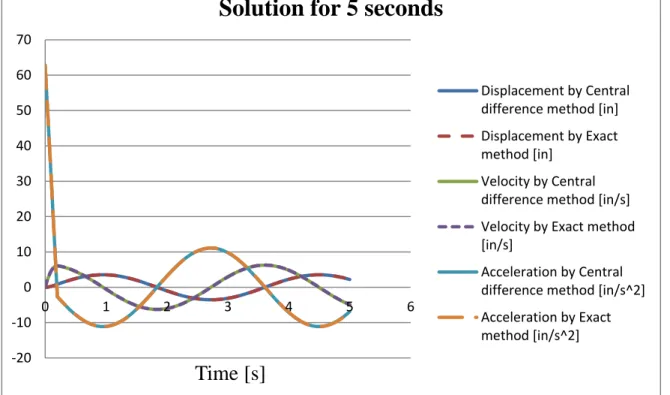
To solve a linear problem with spring-mass which was shown in 4.1.1.1, first the Central difference method is used. Note that and after the time of the is zero. As it was mentioned in the part of introducing central difference method, and ̇ must be known, and both of them are zero in the current problem. So, by implementing the central difference method for the current problem that is a single degree of freedom problem, it can be solved to get displacement, velocity, and acceleration of the system. To see the result, a graph is plotted in the Figure 5-1 in 5s to check out how the displacement, velocity, and acceleration of the system are changed.

Figure 5-1: Results of central difference method for 5 seconds

5.1.1.2. Solution with exact method

To verify the results of 5.1.1.1, this problem has solved with ODE45 in Matlab which gives a very exact solution. In the pictures below, two pictures can be seen. The left one is solution of central difference method, and the right one is the almost exact solution with ODE45 in Matlab.

34

(a) (b)

Figure 5-2: Comparison of results with two methods of central difference and exact method for 5 seconds

It is clear that they are very similar. Also, to have a closer look, first 0.2s of this example is magnified in pictures below, and like the last two pictures, the left one is solution with central difference method and the right one is the exact solution of current problem.

(a) (b)

Figure 5-3: Comparison of results with two methods of central difference and exact method for 0.2 seconds

It should be included that the time step for central difference method in above pictures was

.0.0s but in exact solutions it was 0.005s. By putting two graphs of different solutions together below graph will be obtained.

35

Figure 5-4: Comparison of results with two methods of central difference and exact method for 5 seconds

It is clear that there is not any difference between results of exact method and central difference method. So, the error of central difference method is negligible.

5.1.2. Results of second spring-mass problem

5.1.2.1. Solution with Newmark’s method

In this section, problem of 4.1.1.2 is solved. After 2 seconds the is zero. Like, the problem of 4.1.1.1, and ̇ are zero, and . Lastly, after solving the problem by Newmark’s method, displacement, velocity, and acceleration are calculated, as can be seen in the figure below.

-20 -10 0 10 20 30 40 50 60 70 0 1 2 3 4 5 6

Time [s]

Solution for 5 seconds

Displacement by Central difference method [in] Displacement by Exact method [in]

Velocity by Central difference method [in/s] Velocity by Exact method [in/s]

Acceleration by Central difference method [in/s^2] Acceleration by Exact method [in/s^2]

36

Figure 5-5: Figure 5-1: Results of 4.1.1.2 for 2 seconds

In those two problems that they have solved with two different methods, the parameters were different. In next section, results of a pendulum will be discussed, and it will be solved with both Newmark and central difference method. Then, it would be possible to compare the calculation time and time steps which have used to solve the problem when the same parameters chose to solve the problem.

5.1.2.2. Solution with exact method

To compare the results of Newmark’s method in 5.1.2.1, by exact method, ODE45 of Matlab has used to get the exact solution. In the pictures below, in left side, results of Newmark’s method, and on the right side the exact solution are comparable.

(a) (b)

Figure 5-6: Results of 4.1.1.2 with two methods of central difference and exact method for 2 seconds

37

By putting these two plot on each other, the below graph will be obtained for displacement and velocity of solutions with Newmark and exact method.

Figure 5-7: Comparison of results for 4.1.1.2 with two methods of central difference and exact method for 2 seconds

It is crystal clear that the error between those methods is negligible, and it must be mentioned that time step in Newmark’s method was 0.01s, and in exact method was 0.0001s. More, the Matlab code of exact method which is written by ODE45 in Matlab is available in appendix.

5.2. Results of two degrees of freedom problems

5.2.1. Results of pendulum problems

5.2.1.1. Results of spring pendulum problem

Solution with Newmark’s method

In this part, problem 4.2.1.1 is solved . Therefore, to solve this problem, first the Newmark’s method is performed with . Plus, the matlab code of this example can be found in appendix. The results are available in figures below:

-60 -40 -20 0 20 40 60 80 0 0.5 1 1.5 2 2.5

Time [s]

Solution for 2seconds

Displacement by Newmark's method [in] Displacement by Exact method [in]

Velocity by Newmark's method [in/s]

Velocity by Exact method [in/s] Acceleration by Newmark's method [in/s^2] Acceleration by Exact method [in/s^2]

38 (a) (b) (c) (d) (e) (f)

Figure 5-8: Results of spring pendulum by Newmark’s method

So, there are some points at the time of solving such problems which will be point out. Furthermore, if stiffness matrix used instead of tangent stiffness matrix in calculation of correction , by iteration matrix , then the results will not change, but that will

39

freedom problems. More, as it was mentioned in the algorithm of Newmark’s method for non-linear problems, to calculate iteration matrix , tangent stiffness matrix has used but if iteration matrix , calculated with stiffness matrix which can be found in matrix of equation of motion, the final result would not change. Then, by using stiffness matrix to calculate iteration matrix the result would be the same but the number of Newton-Raphson iterations in each time step is changed, as consequence, and it is changed like the figure below:

Figure 5-9: Number of Newton-Raphson iteration in each time step

In fact, by using tangent stiffness matrix to calculate iteration matrix , number of Newton-Raphson iterations are between 1-2 but by performing stiffness matrix to calculate iteration matrix, the number of Newton-Raphson iterations changed between 2-3. It means more calculation is required to get the same results. Furthermore, it really crucial to use tangent stiffness matrix to calculate the right correction when Newmark’s method is used to solve the problem, specially that can be a reason to save huge time for calculations of large structures.

In the Figure 5-10, change in length of spring is presented. The changes in length of spring show that problem is highly non-linear.

40

Figure 5-10: Change in length of spring pendulum for 20 seconds with Newmark’s method

As the next step, current problem with the same parameters will be solved with explicit method of central difference method with exactly the same time step. Resultantly, the output of both methods can be compared to understand the differences.

Verification of results

In this part, initial condition of on 4.2.1.1 has changed to 1m, and resolved. It is also solved with transient dynamic analysis of ANSYS. To model the problem in ANSYS, element of COMBIN14 has used which is an element to model spring and damper together but the damping assigned as zero. Also, MASS21 element on ANSYS is performed to model the mass element at the end of spring. More, to apply the transient dynamic analysis of ANSYS, three options are available to choose for analysis consisting of full, reduced, and mode superposition method. The full method is the most accurate one among those three methods, and does not need to define master degrees of freedom, and that can capture all types of non-linearities. In this thesis, full method of transient dynamic analysis of ANSYS has been used to verify the results of written Matlab codes because the full method can obtain the most accurate result among three available methods in ANSYS. Moreover, to see more details of transient dynamic analysis of ANSYS, manual of this section must be followed. On the left hand side of Figure 5-11 results of Newmark’s method with written codes on Matlab and on the right hand side results of ANSYS are shown.

41

(a) (b)

(c) (d)

42

(g) (h)

Figure 5-11: Verification of Newmark’s method with transient dynamic analysis of ANSYS for a spring pendulum

That must be noted that in Figure 5-11 in section of (c) and (d) in y direction the results of ANSYS on section (d) has started from 0 to -2m but on part (c), the range started from 1m to -1m. In fact they are the same figures but ANSYS has used relative coordinate on part (d) of Figure 5-11, and one can makes sure that both pictures of (c) and (d) are the same as each other just (c) is plotted with real assigned numbers but (d) is plotted with relative coordinate system.

Solution with central difference method

In the current section, the problem of 4.2.1.1 is solved with central difference method. Again, the Matlab codes are available in the section of appendix. After, by solving that with central difference method, below figures are obtained:

43

(a) (b)

(c) (d)

(e)

Figure 5-12: Results of spring pendulum by central difference method

Thus, it can be seen that the results are somehow the same, and the time step in both methods were 0.03s. In central difference method, Newton-Raphson itereation is not used. When, Newmark’s method is used to solve the problem the elapsed time was 0.052596s but in case of using central difference method the time was 0.011891s. So, by performing the same time step, central difference method is more than four times faster than Newmark’s method in this special case. However, the trajectory is not exactly the same, and the accuracy of central difference method can increase by choosing smaller time steps which spend more time to calculate the displacements, velocities, and accelerations. Also, the change of length versus time is plotted in Figure 5-13.

44

Figure 5-13: Change in length of spring for 20 seconds with central difference method

In the picture below, the difference in change of spring’s length versus time has been compared between solutions of Newmark’s method, and central difference method. It can be seen that in the first 10 seconds they are somehow the same but after 10 seconds they started to deviate from each other.

Figure 5-14: Comparison of changes in length of spring pendulum with Newmark and central difference method

0 0.5 1 1.5 2 2.5 0 5 10 15 20 25 Leng th of spring [m ] time [s]

Change in length of spring for elastic pendulum

Solution with Newmark's method Solution with central difference method