Analogue versus digital solution for motor control

Analogue versus digital solution for motor

control

Analog versus digital lösning för

motorstyrning

Andreas Johansson

Max Stigborg

Bachelor Thesis 2013

ELECTRICAL ENGINEERING

This thesis has been carried out at the School of Engineering in

Jönköping within the subject of Electronic design. The work is a part of the three year bachelor education. The authors take full responsibility for presented opinions, conclusions and results.

Examiner: Anders Adlemo

Mentors: Mats Johansson, Ingemar Thöörn och Jonas Nordqvist, Saab AB i Jönköping.

Magnus Schoultz, Jönköpings Tekniska Högskola.

Scope: 15 credits (bachelor)

Abstract

Saab has an analogue solution which is used to drive small motors in aircrafts. The motor is a brushless DC-motor and uses a resolver and hall sensors to control it. As sensorless control is something that has been expanding and attracting more interest over the last decade, Saab is considering the possibility of using a digital sensorless system depending on its performance on the control compared to their analogue system.

There is little documentation of performance for a digital sensorless solution compared to an analogue solution. Therefore the question to be answered in this research is: How is the performance of the digital solution compared to the existing analogue

solution?

It was answered by finding a complete sensorless system on the market and then compare its performance to a digital system with sensors that resembles the analogue solution.

Performance wise, InstaSPIN does not perform as well as EPOS2 which represent the sensorless system respective the system with sensors. InstaSPIN needs a startup sequence, can not run at the same low velocities, has a longer rise time, settling time and greater ripple. An examination of the software should be done before using the disadvantages that was found as a reason for not

considering a sensorless system. Especially the startup sequence in the software should be examined as it is InstaSPINs greatest weakness compared to EPOS2.

Keywords

Sammanfattning

Saab använder idag ett analogt system för att driva små motorer i deras flygfarkoster. Det analoga systemet använder en borstlös DC-motor och en resolver för styrning av motorn. Motorstyrning med system som är oberoende av givare är ett område som vuxit och fått ett ökat intresse det senaste decenniet. Saab överväger möjligheten att använda ett givarlöst digitalt system beroende på dess styrprestanda jämfört med deras analoga system.

Eftersom det finns lite dokumentation om prestandan så är frågan som ska besvaras i denna rapport: Hur förhåller sig det givarlösa digitala systemet prestandamässigt

jämfört med det existerande analoga systemet?

Detta besvarades genom att leta upp ett komplett system på marknaden och sedan jämföra dess prestanda mot ett digitalt system som liknar det analoga systemet. Prestandamässigt så fungerar InstaSPIN som representerar det givarlösa systemet inte lika effektivt som EPOS2 som representerar systemet som använder givare. Nackdelarna med InstaSPIN är att den behöver en startsekvens, inte kan köra på lika låga hastigheter, har längre stigtid, insvängningstid och större rippel. Man bör undersöka mjukvaran innan nackdelarna används som en anledning till att inte använda ett givarlöst system. Speciellt startsekvensen bör undersökas eftersom det är IntaSPINs största svaghet jämfört mot EPOS2.

Abbreviations and explanations

BEMF Back Electromotive Force BLDC Brushless DC-motor

CV Current and Velocity regulator EC Electronically Commutated EDS Electronic Defence System

PMSM Permanent Magnet Synchronous Motor

RES Ramp End Speed

RSS Ramp Start Speed

SC Startup Current

Table of contents

1

Introduction ... 1

2

Theoretical background ... 4

2.4.2 The startup procedure ... 10

2.5 BACK ELECTROMOTIVE FORCE ... 11

2.5.1 Other BEMF Sensing Techniques ... 13

2.6 ZERO CROSSING DETECTION ... 13

3

Method and implementation ... 15

3.1 LITERATURE STUDY ... 15

3.2 MEETINGS ... 15

3.3 EQUIPMENT AND SETUP ... 16

3.3.1 Selection of development kit ... 16

3.3.2 EPOS2 ... 16

3.3.3 Maxon motor ... 17

3.3.4 The configuration and setup of the software and hardware ... 17

3.4 TEST PHASES ... 18

3.4.1 Test phase - PI Values ... 19

3.4.2 Test phase - Startup Control ... 20

3.4.3 Test phase - Reliability ... 20

3.4.4 Test phase - Optimal step response at lowest stable velocity ... 21

3.4.5 Test phase - Step response and Distance ... 22

3.4.6 Test phase - Ripple and Transitions at lowest velocity ... 22

3.5 COMPARISON ... 23

4

Results and analysis ... 24

4.1 TEST PHASE -PIVALUES ... 24

4.1.1 EPOS2 Auto tuning ... 24

4.1.2 Comparison of PI-gain amplifications at 480 and 1020 rpm ... 24

4.1.3 Comparison of PI-gain amplifications at 1500 and 1980 rpm ... 26

4.2 TEST PHASE -STARTUP CONTROL ... 28

4.2.1 Comparison of the Start Ramp Time ... 28

4.2.2 Comparison of the Startup Current ... 28

4.2.3 Comparison of combinations of RSS and RES ... 30

4.3 TEST PHASE -RELIABILITY ... 31

5

Discussions and conclusions ... 45

5.1 DISCUSSION OF THE RESULT ... 45

5.1.1 The performance on the startup sequence in the matter of rise time and settling time from zero to lowest stable velocity ... 45

5.1.2 The settling time from a set velocity to the lowest stable velocity... 46

5.1.3 The standard deviation of the ripple at a low constant velocity ... 46

5.1.4 Related studies ... 46

5.2 DISCUSSION OF THE METHOD ... 47

5.3 LITERATURE STUDY ... 47

5.4 TESTS ... 47

5.5 CONCLUSIONS AND FUTURE WORK ... 48

6

References ... 50

7

Appendix ... 52

7.1 APPENDIX 1:A MORE PRECISE COMPARISON OF THE PI-GAIN VALUES ... 52

7.2 APPENDIX 2:COMPARISON FROM THE SECOND RUN BETWEEN THE DIFFERENT COMBINATIONS OF STEP RESPONSES AT 420 RPM AND 1260 RPM WITH A SMALL LOAD RESPECTIVE HEAVY LOAD. ... 53

List of figures

FIGURE 1:MODEL OF A DC-MOTOR [20] ... 4

FIGURE 2:MODEL OF A 3-PHASE BRUSHLESS DC-MOTOR WITH 2 POLES ... 5

FIGURE 3:THE COMMUTATION LOGIC FOR A BLDC-MOTOR [13] ... 6

FIGURE 4:HALL 1 SENSOR OUTPUT IS 1 AND THE RESULT PATTERN IS 001 ... 7

FIGURE 5:HALL 1 AND HALL 2 SENSORS OUTPUT IS 1 AND THE PATTERN IS 011 ... 7

FIGURE 6:THE THREE PHASES DRIVEN HIGH AND LOW OVER THE SIX STEPS.THE THREE LOWER SHOWING HOW THE VOLTAGE WILL LOOK BECAUSE THE BEMF.THE SPIKES ARE DRAWBACKS FROM THE COILS WHEN THEY DE-ENERGIZE. ... 12

FIGURE 7:THE VOLTAGE OVER THE THREE PHASES, THE ZERO CROSSING FOR BEMF AND THE DESIRED FLUX ... 14

FIGURE 8:SCHEMATIC OF TEST PHASES ... 18

FIGURE 9:GRAPH OF STEP RESPONSES AT 480 RPM USING A SMALL LOAD ... 25

FIGURE 10:GRAPH OF STEP RESPONSES AT 1020 RPM USING A SMALL LOAD ... 25

FIGURE 11:GRAPH OF STEP RESPONSES AT 1500 RPM USING A SMALL LOAD ... 26

FIGURE 12:GRAPH OF STEP RESPONSES AT 1980 RPM USING A SMALL LOAD ... 27

FIGURE 13:COMPARISON OF SRT VALUE BETWEEN 1 MS AND 1000 MS ... 28

FIGURE 14:GRAPH SHOWING THE COMPARISON OF THE STARTUP CURRENT PARAMETERS AT 780 RPM. 29 FIGURE 15:GRAPH SHOWING THE COMPARISON OF THE STARTUP CURRENT PARAMETERS AT 1020 RPM 29 FIGURE 16:THE DIFFERENCE BETWEEN THE VARIOUS COMBINATIONS OF RSS AND RES AT 780 RPM .... 30

FIGURE 17:THE DIFFERENCE BETWEEN THE VARIOUS COMBINATIONS OF RSS AND RES AT 1020 RPM .. 31

FIGURE 18:COMPARISON FROM THE FIRST RUN BETWEEN THE DIFFERENT STEP RESPONSES AT 420 RPM WITH A SMALL LOAD ... 34

FIGURE 19:COMPARISON FROM THE FIRST RUN BETWEEN THE DIFFERENT STEP RESPONSES AT 1260 RPM WITH A HEAVY LOAD ... 34

FIGURE 20:THE STEP RESPONSE OF INSTASPIN AND EPOS2 FROM 0 TO 420 RPM WITH A SMALL LOAD. 36 FIGURE 21:THE REVOLUTIONS DURING THE STEP RESPONSE FOR INSTASPIN AND EPOS2 AT 420 RPM . 36 FIGURE 22:A CLOSER LOOK AT THE REVOLUTIONS AT THE BEGINNING OF THE MOTOR ROTATION AT 420 RPM. ... 37

FIGURE 23:STEP RESPONSE FOR INSTASPIN AND EPOS2 FROM 0 RPM TO 1260 RPM WITH HEAVY LOAD ... 37

FIGURE 24:THE REVOLUTIONS DURING THE STEP RESPONSE FOR INSTASPIN AND EPOS2 AT 1260 RPM 38 FIGURE 25:A CLOSER LOOK AT THE REVOLUTIONS AT THE BEGINNING OF THE MOTOR ROTATION AT 1260 RPM. ... 38

FIGURE 26:THE TRANSITION FROM 240 TO 180 RPM USING A SMALL LOAD ... 40

FIGURE 27:THE TRANSITION FROM 300 TO 240 RPM USING A SMALL LOAD ... 40

FIGURE 28:THE TRANSITION FROM 480 TO 420 RPM USING A HEAVY LOAD ... 41

FIGURE 29:THE TRANSITION FROM 560 TO 480 RPM USING A HEAVY LOAD ... 41

FIGURE 30:THE COMPARISON OF RIPPLE AT 180 RPM WITH A SMALL LOAD ... 42

FIGURE 31:THE COMPARISON OF RIPPLE AT 240 RPM WITH A SMALL LOAD ... 43

FIGURE 32:THE COMPARISON OF RIPPLE AT 420 RPM WITH A HEAVY LOAD ... 43

List of tables

TABLE 1:MOTOR DRIVE TABLE FOR A BLDC MOTOR FOR A CLOCKWISE DIRECTION ... 7

TABLE 2:THE PI-GAIN VALUES OF EPOS2 AND INSTASPIN ... 24

TABLE 3:THE RISE TIMES FROM 0 TO 70% OF THE DEMAND VALUE AT 480 AND 1020 RPM ... 26

TABLE 4:THE RISE TIMES FROM 0 TO 70% OF THE DEMAND VALUE AT 1500 AND 1980 RPM ... 27

TABLE 5:THE PREVIOUS AND THE PRESENT PI-GAIN VALUES FOR THE REGULATORS IN THE INSTASPIN SOLUTION ... 27

TABLE 6:TABLE SHOWING HOW THE FAIL RATE WAS RATED ... 31

TABLE 7:THE RELIABILITY AT 360 RPM WITH A SMALL LOAD ... 32

TABLE 8:THE RELIABILITY AT 420 RPM WITH A SMALL LOAD ... 32

TABLE 9:THE RELIABILITY AT 1200 RPM WITH A HEAVY LOAD ... 32

TABLE 10:THE RELIABILITY AT 1260 RPM WITH A HEAVY LOAD ... 33

TABLE 11:THE LOWEST STABLE VELOCITIES FOR SMALL AND HEAVY LOAD TOGETHER WITH THE OPTIMISED PARAMETERS. ... 35

1 Introduction

The most common way of controlling an electric motor is with the help of sensors. This can however be achieved without sensors as there are several new techniques available on the market.

At Saab a BLDC-motor is used in a project to control a throttle lever in an aircraft. The solution for the motor control is analogue and uses a resolver as a sensor to control it. The system is robust and reliable but it may be improved in safety by removing components such as sensors and therefore making it

sensorless.

By comparing a sensorless digital system to a system with sensors, Saab will gain knowledge in the performance of the sensorless solution. This work is a part of the Electronic design program at the School of Engineering in Jönköping and was requested by the Avionics department at Saab Electronic Defence System in Jönköping.

1.1 Background

Saab has developed different control systems, both digital and analogue, for BLDC-motors. For small motors, an analogue control has been developed. It is robust and working but Saab is looking for another improved way of controlling the motor digitally without sensors. By removing the sensors there are fewer components that may cause problems which is considered a safety and reliability improvement of the present system. Sensorless control is something that has been expanding and attracting more interest over the last decade and due to that it may be used as a solution. Since Saab have limited experience of sensorless control, it became our task to analyse and evaluate it.

This has not been done before because the digital electronic requires very high development and validation costs which include certification and procedures needed to get it validated for use. If this thesis proves that the sensorless solution performs well, a further analysis would be executed and it may be implemented in the future. So this research is going to cover a study and evaluation of a sensorless solution by comparing it to the digital system that resembles the existing analogue solution.

1.2 Aim and Purpose

The purpose of this thesis is that Saab wants to learn more about controlling a sensorless BLDC motor and its performance compared to the digital solution that resembles their analogue system.

The main problem to be solved in this paper can be summarised as:

- How is the performance of the digital solution compared to the existing analogue solution?

To narrow down the problem, it can be divided into different sub questions: - What is the performance on the startup sequence in the matter of rise time

and settling time from zero to lowest stable velocity?

- How is the standard deviation of the ripple at a low constant velocity? - How is the settling time from a set velocity to the lowest stable velocity?

1.3 Method

In order to solve the problems, the first part involves gathering information about the existing sensorless solutions on the market. It was decided to select two

solutions, one as main and the other as backup. The two solutions were selected based on their specifications for instance concerning its CPU type, temperature range and development possibilities. After studying the main one, tests was performed together with an analysis of the performance. It was then compared in the matter of the rise time, settling time and ripple to a system resembling Saab's existing one.

1.4 Limitations

This thesis will only focus on one sensorless BLDC-control solution and only mention other theoretical ones. This report will not explain technically how the analogue solution works since it is already documented. There will be no software coding or attempts to improve the existing code because it is too complex and would consume too much time.

The performance will only be tested at different velocities ranging from 1 rpm up to 2000 rpm. The number of tests on each phase will be restricted due to time restraints. The only motor used for testing was supplied from Saab and it ranges from 20 to 48 V and up to 100 W. A load simulator was hooked on at all times but was only used in two different modes, heavy load and small load.

1.5 Outline

The report is divided into a total of 4 chapters: theoretical background, method and implementation, results and analysis together with discussions and

conclusions.

Method and implementation explains which methods that have been used in this

analysis. This chapter contains a description on how information was gathered together with how meetings, tests and analysis were implemented.

In Results and analysis all the results from the performed tests are presented in

graphs and tables. In this part, the analysis of the paper can be found.

The Discussion and conclusions chapter includes the discussion of the method and the

results presented in the previous part. This discussion will include how the purpose and the questions have been fulfilled and answered.

2 Theoretical background

The theoretical background describes the basics of the electrical motor and how it is controlled. It also describes the sensorless method that InstaSPIN solution is using along with other sensorless methods.

2.1 DC-motor

The most common DC-motor motor used is a brushed DC-motor. In figure 1, a DC-motor can be seen. From the outside to the inside it consists of a permanent magnet surrounding a rotor which is free to spin. The rotor consists of three electromagnets and the commutator. It is the commutator that are in contact with the brushes that supply the voltage and from the brushes to the electromagnets [8].

Figure 1: Model of a DC-motor [20]

When electricity runs through the electromagnet they will generate a magnetic field around them. The magnetic field will cause the rotor to repel and attract the poles of the surrounding permanent magnet. Since the permanent magnet can not move, the rotor will rotate making the fields align. When the rotor reach a set position a commutation will occur and then the commutators will come in contact with the next brushes changing the polarity of the electromagnet and the position of the magnetic fields.

The benefits with this kind of construction are the simplicity and the low price due to low manufacturing costs. Almost all the negative aspects are related to the brushes, which may wear out; generate static noises, limit the speed and the number of poles the rotor can have. Another type of drawback is the problem of

2.2 Brushless DC-Motor

The brushless DC-motor has permanent magnets on the rotor and the

electromagnets are placed on the stator as seen in figure 2. The electromagnets will then be charged up using electronic control. When they are energised correctly the rotor will spin and the direction can be easily controlled if the position of the permanent magnets is known [5].

Figure 2: Model of a 3-phase brushless DC-motor with 2 poles

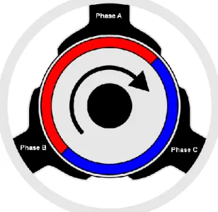
In order to drive a BLDC-motor an electronic commutation logic together with a sensor are required. These can solve the two problems about the commutation and speed control as the logic replaces the function of the brushes and the sensor determines the position of the rotor. The commutation logic consists of six transistors that can be turned on and off, which can be seen in figure 3. The motor is driven by pulses of voltage that depends on the position of the rotor. The pulses should be properly applied to the active phases so the angle between the stator flux and the rotor flux is as close to 90 degrees to obtain the maximum torque. The speed of the motor can be controlled by adjusting the rotor voltage and current. This is because the speed relies on the strength of the magnetic field that is generated by the energised coils which depends on the current through them [3].

Figure 3: The commutation logic for a BLDC-motor [13]

The advantages over brushed dc-motors are, longer lifetime due to no brushes and commutator erosion. Another benefit is that there are no sparks from the commutator and there is a reduced electrical noise.

2.3 Sensored control

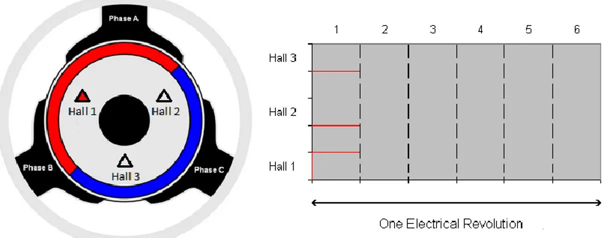
There are different methods of controlling a BLDC-motor and the simplest way to do so is by the trapezoidal commutation using hall effect sensors. With trapezoidal (six-step) commutation there are two or three phases that receive current depending on the hall effect sensors state. In trapezoidal commutation, the electrical revolution is divided into six steps of 60 degrees each, hence the name six-step. The speed can be controlled by varying the voltage across the motor [3].

In order for proper commutation and motor rotation the rotor position has to be known. By using hall effect sensors the position of the rotor can be determined. With the rotor position known the electrical switches in the electronic

commutation logic can be turned on and off to ensure the proper current flow in respective coils. The hall effect sensors are usually placed 120 degrees apart and give an “1” as output whenever the north pole of the rotor faces the sensor or vice versa depending on which configuration is set on the sensors [13].

With the three hall effect sensors combined it will create a 3-bit binary word which is generated from the output of the sensors. The information how these 3-bit binary words can be used to control the motor is generally provided in the motor datasheet. It is usually in a form of a diagram or a table that shows which phases that should be set to, High, Low or Off depending from the 3-bit binary word that is given from the hall effect sensors which can be seen in figure 3 [15]. In figure 4, it shows the first step how hall effect sensors work on a two pole

Figure 4: Hall 1 sensor output is 1 and the result pattern is 001

At the next step the output from the hall effect sensors is 011 shown in figure 5. The phases Phase A, Phase B, Phase C are respectively set to Low, High and Off in order for a continued clockwise rotation.

Figure 5: Hall 1 and Hall 2 sensors output is 1 and the pattern is 011

The pattern that is used for a clockwise rotation is presented in table 1.

2.3.1 Resolver

A resolver is a transducer that can measure the instantaneous angular position of the shaft that is attached to its rotor. It can be used for commutation or be used for speed control. The construction of the resolver are typically built like small electrical motors. The resolver consists of a stator with two coils that are

perpendicular to each other. Inside the stator there is a rotor with a coil called the reference coil [2].

In order to measure the rotors angular position, an AC voltage (Vr) with a

frequency of 1-20kHz has to be applied over the reference coil. This will result in that the other coils will generate a sinus respective a cosine signal by the excited voltage.

The Sin and Cos coils induced voltage are equal to the reference voltage

multiplied by the sin or cos of the angle of the input shaft from a fixed point. This gives us the formulas:

 

 

Vs = Sin Induced Voltage. Vc = Cos Induced Voltage. Vr = Reference Voltage.

T = Transformation ratio (max output voltage / input voltage).

The ratio between the two voltages represents the absolute position of the rotor:

 

 

 

Were θ = rotors angle

The rotors angle can be solved by using this formula:

 

 

The angle of the rotor is a unique combination of sine and cosine values and since every angle have a unique combination thus makes it an absolute position sensor which means that it has a very high accuracy.

With the ratio between sin and cos the resolver is not dependent on changes of its characteristics such as those caused by time or temperature changes. Another advantage is that when the power is removed and the rotor has been rotated, the resolver will report the new position when the power is restored [2].

2.3.2 Encoder

Encoders are electromechanical transducers which output is obtained by reading a coded pattern on a rotating disk. There are two types of encoders, absolute or incremental.

The absolute encoder is measuring the current position of the rotor which makes it an angle transducer. The incremental encoder is measuring the motion of the rotor which can be used to calculate speed, distance and position. There are two methods used to read the coded element, contact or non-contact [16].

2.4 Sensorless Control

The InstaSPIN-BLDC is a solution from Texas Instruments for controlling a sensorless BLDC-motor. The solution is built on the six-step trapezoidal control commonly used with BLDC-motors using sensors. This solution replaces sensors with measuring the voltage output of the electromagnets on the motor which is known as back electromotive force (BEMF). The technique is based on the permanent magnet with its flux used as a rotor. The flux that rotates induces a voltage in the surrounding electromagnets. The voltage will differentiate as the rotor spins and the magnetic field moves [19].

The voltage is measured on the non used phase to calculate the flux when the voltage goes from positive to negative or the other way. When the flux has

reached the desired level the commutation occurs and it starts waiting for the next zero crossing to start on the next phase. This method differs from other zero crossing methods where the time is measured between the two latest zero crossings and predicts the next commutation based on the half of time that was measured. The difference in performance comes down to that InstaSPIN-BLDC handles the velocity changes better since it works with real time values instead of predicting values.

The solution uses two PI-regulators which operate in different ways based on the four modes this solution can be run in. The first mode is called Duty Cycle where it doesn’t use any of the regulators and runs an open-loop duty cycle. The second is Current mode where it only uses the current PI-regulator. The third mode is Velocity mode which only uses the velocity PI-regulator. The last is Cascade mode which uses both PI-regulators for both controlling the velocity and current.

2.4.1 InstaSPIN GUI

The DRV8312 kit includes a program called Control suite which contains code examples, user guides and other free information. With the InstaSPIN-BLDC solution a pre-programmed graphical user interface (GUI) is included. It is a program made to set the parameters for the system and observe its performance. The GUI gives the user information about the supplied voltage, supplied current, velocity, BEMF on phase A, integrated motor flux and current waveform on motor phase A. The setup page contains five different setup categories: Startup Control, Advanced Startup Options, Current Loop, Velocity Loop and Motor Parameters [18].

In Startup control, parameters can be set to control how the motor initially ramps up under forced commutation. The parameters are the following,

- Startup Current (SC) - Sets the current limit in the startup sequence. - Start Ramp Time (SRT) - The time taken to complete the forced

commutation ramp up phase.

- Ramp Start Speed (RSS) - The initial speed for the forced commutation ramp up phase.

- Ramp End Speed (RES) - The final speed for the forced commutation ramp up phase.

Advanced Startup Options contains optional parameters for the commutation events

under the startup sequence.

Current Loop contains the parameters for the current loop which is only active in

Current Mode or Cascade Mode.

Velocity Loop operates the parameters for velocity PI-regulator.

Motor Parameters sets up information about the number of poles used and base

electrical frequency [18].

2.4.2 The startup procedure

InstaSPIN does not use any alignment or position algorithm in its startup

sequence. Instead it starts with commutating according to a pattern and reads the BEMF if it spins in the right direction. If it reads that the BEMF is wrong it will jump to another step in the six step process. After reading the right direction with several successful commutations it discards the startup procedure and starts using the general BEMF sensing technique [4].

2.5 Back Electromotive Force

Back electromotive force commonly known as BEMF which is the induced voltage in electromagnets and works to prevent the movement of magnetic field. The BEMF technique is based on Lenz Law about inducing current [1]. Lenz law states that the current generated through electromagnetic induction works to oppose its source by generating a magnetic field in the opposite direction to the current one [14]. The BEMF is then sent back to microcontroller for the desired operation.

The BEMF is measured in volts and its strength depends on the: - Number of turns of coil windings.

- Angular velocity of the rotor. - Magnetic field generated. - Length of the rotor. - Internal radius of rotor.

Summarizing this to one formula gives: w B r l N BEMF      (2.5) N = number of windings l = Length of rotor

r = Internal radius of the rotor B = Rotor magnetic field w = Angular velocity

As the four first are constants it leads to the conclusion that the BEMF is directly proportional to angular velocity [1].

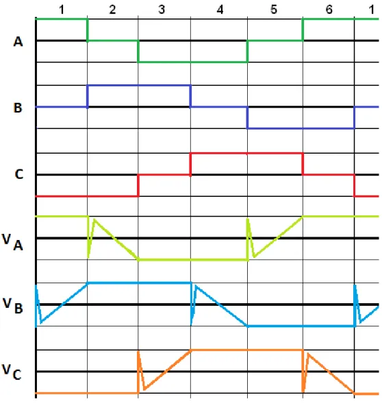
Figure 6 show that when two phases are driven high and low the third phase that should be zero V is actually increasing or decreasing because of the BEMF generated at that moment.

Figure 6: The three phases driven high and low over the six steps. The three lower showing how the voltage will look because the BEMF. The spikes are

drawbacks from the coils when they de-energize.

The drawback that comes with this method is that the motor will not start when the supply voltage is lower than BEMF generated. It does not give a reading when standing still and a poor reading at low speeds. The sudden commutation have one drawback, as there is a voltage over the windings when a commutation occur [1], coils work in such manner that when they are interrupted a sudden voltage spike is created. This is overcome by discarding the first samples after a

2.5.1 Other BEMF Sensing Techniques

There are generally two categories of sensing the BEMF, direct and indirect BEMF-sensing, these categories are further divided into a total of five general methods. The direct BEMF detection consists of the two groups, Zero Crossing Detection and PWM strategies. The indirect BEMF detection methods are divided into BEMF Integration, Third Harmonic Voltage Integration and Free-wheeling Diode Conduction.

The main differences between direct and indirect are the high common mode and high frequency noise due to the PWM drive that is used in the direct category. To prevent them one has to use low-pass filters and voltage dividers which causes delays for the commutation timing at high speeds and reduced signal sensitivity at low velocities because of attenuation [7].

The stators are meant to make trapezoidal BEMF as close looking to the supplied voltage as possible. Unfortunately this is considered very difficult to do in reality and the BEMF signal often looks more like a sinusoidal signal than a trapezoidal signal. This makes it possible to use many of the control techniques used in permanent magnet synchronous motor (PMSM) control [17].

2.6 Zero Crossing Detection

Zero crossing is referred to when the BEMF passes the neutral point when increasing or decreasing. The neutral point is calculated by measuring the voltage on the phases and calculates an average value [1]. In the BLDC-motor solution the observed zero crossing is the voltage on the non-supplied phase [6]. When it comes to InstaSPIN it diverges a bit from what is regularly done with the BEMF signal.

In regular zero crossing the time is measured from last zero crossing to next one. The time is divided by two and used as time base for when the next commutation should occur. This solution works well at constant velocity but not very well when the velocity changes. The reason is due to the solution is based on predicting the commutation point. If the speed is suddenly changed it will miss the commutation time and will suffer a torque drop. This case can be ignored depending on the use of the solution [6].

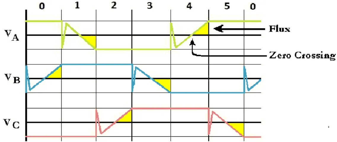
When it comes to timing the commutations this is where InstaSPIN excels the regular zero crossing method. InstaSPIN calculates the flux in real time repeatedly for when it reaches a set values to commutate. Flux is the integration from

voltage, choosing where to start measuring and repeatedly measuring its actual value will give a very precise commutation timing which can be seen in figure 7[6].

Figure 7: The voltage over the three phases, the zero crossing for BEMF and the desired flux

The flux is calculated by:

dt d N

V



N= Number of turns in Coils θ = Flux

V =Voltage

a = Zero crossing point for voltage. b = BEMF

Another positive effect of integration is that an integrator is a low pass filter, so even if there is ripple on the voltage this can be neglected and will not affect the commutation timing [6]. To avoid the wrong zero crossing that occurs right after commutation the system discards the first couple of measurements [1].

3 Method and implementation

The method and implementation describes the approach of solving the main problem:

How is the performance of the digital solution compared to the existing analogue solution?

This was solved by gathering information from existing sensorless systems on the market followed by a selection of two complete systems. One of them was

chosen, studied and tested for its performance. The performance was then compared to a system resembling Saab’s existing one.

Before this assignment was accepted, it was specified that the first part included design and construction of a developer board. The developer board was meant to operate with a sensorless BLDC-motor. On the first meeting the assignment was changed due to time restraints, the task was now to find a developer board meeting the desired requirements.

3.1 Literature study

During the project theoretical information was gathered simultaneously. The goal was to learn and study the different sensorless techniques. The information was collected from different sources as listed below:

- Literature from the university library in Jönköping. - Google scholar for associated articles and reports.

- Datasheets for the concerned components, items and solutions from the manufacturer.

Even if most of the sources were articles or application notes taken directly from the manufactures, they were compared to other sources to confirm that the information was reliable.

3.2 Meetings

The meetings were held frequently with the Saab’s supervisors. At the meetings, the progress was discussed in the matter of what had been done and what

problems had occurred. To help Saab understand the progress since the previous meeting, the latest test results were presented together with questions related to the result. After resolving and processing the problems, there was a discussion about what the next step would be. The meetings were considered a part of the work because they were found useful to the project, due to the solving of upcoming problems and questions which occurred during the project.

3.3 Equipment and setup

3.3.1 Selection of development kit

The first part of the work was to select a developer kit. At a meeting it was decided to choose one as main and a second as backup if problems would occur with the main kit such as too long delivery time. The boards were chosen based on temperature range, type of processor, board specifications, familiarity with the processor family and possible use of the processor in the future. It should also be a complete kit which means it should be included with source code that can run directly without any programming.

DRV8312-kit from Texas Instruments was chosen as the main kit and 3-phase Sensorless BLDC-Kit from Freescale as backup. The DRV8312-kit was chosen because of the floating point processor, development possibilities, included source code and software. As well as because of a suitable temperature range was found in the same processor family and an interest of the processor due to old projects has been using Texas Instruments processors. As the delivery time was too long on the Freescale kit a new secondary was needed, a developer board named dsPICDEM MCLV-2 from Microchip was chosen.

3.3.2 EPOS2

To simulate the analogue system an electronic device called EPOS2 was used. It is used for connecting DC-motors to a software called EPOS Studio for motor control and performance measurements. The solution is initiated with connecting the desired motor and its sensors to EPOS2 and moving the jumpers for the right motor setup. The setup differs depending on which sensors to use, what kind of motor and what is controlling the motor. In the software it was required to run a startup wizard and fill in necessary information about the setup. The required data was for instance motor type, motor specifications, commutation and sensor. The motor specifications included maximum permissible speed, nominal current, thermal time constant of motor winding and pole pairs. The next step was setting the resolution for the encoder and the safety parameters.

When the motor is connected to the EPOS2 board the PI values can either be set manually in the expert tuning or by using the auto tuning feature in EPOS Studio. The auto tuning will automatically calculate the optimal PI values for the motor and in the expert tuning the values can be set manually.

To observe the motor performance, it is shown in the data recording tool which can be configured for the desired information. It can handle up to four data channels at the same time. The amount of samples is always fixed for the graph and together with sampling frequency which decides the time period. It can show 17 different signals for instance demand values, average, errors and sensor

3.3.3 Maxon motor

The motor used in this project was a Maxon EC-4pole 30 Ø30mm brushless 100 Watt. Its max velocity rated at 25000 rpm and the maximum voltage is 48 V with a torque constant of 25.5 mNm/A. It is a three phase motor with two pole pairs [10]. An encoder is mounted on the end of the motor it is also from Maxon motors and has a resolution of 1000 counts per turn. It got three channels and is capable of handling velocities up to 12000 rpm [11]. On the other side there is a planetary gearhead with a reduction of 246:1, in this report the gearheads rotor will not be measured [12].

3.3.4 The configuration and setup of the software and hardware

The next part consisted of configuration of the boards and the software, also to connect the motor with the load. To get the best regulation the motor was

connected to the EPOS2 board and was running using the Hall effect sensors and recorded the step response with the encoder.

The load setup was done by attaching the motor to a metal piece that prevented the motor from rotating when a load was connected to the motor. The metal piece was then attached to a table using a clamp. The load contains of a rotor attached to a flat and heavy metal piece. In order to create a regulated force to the rotor, a crescent formed metal piece with two springs was placed under the rotor. The load was regulated by the springs which can be adjusted. By adjusting the screws it made the spring’s contract or release causing more or less force to be applied on the rotor. With the springs completely screwed down there is no force applied to the rotor and only the rotor itself acts as a load, this will be called a small load. As for the heavy load it is when springs are turned down at all. The load is attached to the table and the motor.

Since the motor and the load were not attached to the same metal construction some glitches occured. For instance when the motor tried to spin with a heavy load it turned the load construction just for a bit before actually spinning the rotor on the load. This might have some effect on the results of the tests.

There are four values that need to be converted to work with the InstaSPIN solution, P-gain and I-gain for the current respective velocity regulation. The values may not be optimal for InstaSPIN but the ratio between P-gain and I-gain should remain the same. Since it is not known if the calculated values are optimal for the InstaSPIN solution, tests were performed with different PI values but still maintained the same ratio.

3.4 Test phases

This subchapter describes the method of the performed tests. The tests were divided in different test phases, this was to organise and simplify the tests. The test schematic that displays in what order the test phases were performed are presented in figure 8.

The tests are shown in green boxes, results in white, performed actions in blue and data in yellow. The data are obtained from an analysis of the results which were later used in the application.

3.4.1 Test phase - PI Values

The purpose of this phase was to find PI values that created an optimal step response in the matter of rise time and settling time before comparing it to the EPOS2 system.

The auto tuning in EPOS2 was performed and the PI values were collected and converted to be used in the InstaSPIN solution. The values were implemented in the interface and the motor phases were connected to the DRV8312-C2-KIT for manual testing. EPOS2 was active and EPOS Studio was set to data recording with velocity actual value as active. There are two ways to view the velocity;

- The InstaSPIN GUI which shows the velocity calculated by BEMF voltage.

- The data recorder in EPOS Studio, which display the velocity measured by the encoder.

The two results were compared and the InstaSPIN GUI was found to be not as accurate as the encoder. It was decided to only compare the encoder’s value of velocity.

During the testing phases, two computer monitors were used. The monitors were displaying the InstaSPIN interface and the EPOS2 data recorder. This was proven to be very useful due to the two windows that had to be displayed were in full screen. Another useful tool used was the macro recorder software, which records mouse clicks and movements. In this software several scripts were made to automate and simplify the testing phases for instance, setting parameters, store recorded data, start and run the motor and the recording of data.

The tests were performed with an amplification of 0.25, 0.5, 1, 2, 4 and 6 of the PI values on both Current and Velocity. Different velocities were also used for the different amplifications, the velocities started from 0 rpm up to 480 rpm, 780 rpm, 1020 rpm, 1500 rpm, 1980 rpm and 3000 rpm.

The reason the velocities are not 500, 750, 1000, 1500, 2000 and 3000 is because of the input for the velocity. The GUI input for the velocity does not directly apply the value of the demanded velocity but instead it uses a scaling format which is not accurate enough. The scaling is in Per Unit (PU) and the accuracy is with 2 decimals. If the input value is for instance 0.08 PU the speed was calculated with the formula:

 





Were N is the base electrical frequency, P is the number of poles on the motor and PU the Per Unit value.

In this case with 0.08 PU the velocity is 480 rpm, this makes every hundredth part 60 rpm and therefore the demanded velocity can never be 500, 750, 1000 or 2000.

In the end the different PI values was summarized for each velocity in a graph showing the improvement and worsening of the different amplifications. The result led to further testing such as 1.25, 1.5, 2.5, and 3 for an even more accurate regulation.

With the help of Saab, a pattern was discovered in the test graphs were PI was compared and theories of improving the step response was created for 1020 rpm. The theories involved for instance increasing the P-gain and decreasing the I-gain in the Velocity regulator which was proven to improve the step response when it was tested. Even though the ratio of the PI values was not maintained the step response was suitable. The decided PI values were stored and used in the other test phases.

3.4.2 Test phase - Startup Control

The purpose of this test phase was to find how the startup control parameters affects the startup sequence then to set them to the best possible value.

The startup control contains the characteristic parameters used to control how the motor initially ramps up under forced commutation. In order to run the motor sensorless BEMF needs to be generated, this is done by initially forcing the motor to spin and then switch to sensorless once there is a clear signal of the BEMF. The first parameter that was tested in Startup Control was Startup Ramp Time (SRT). The SRT is the time taken to complete the forced commutation ramp up phase.The tests were performed with values of 1 ms and 1000 ms at a velocity of 1020 rpm. The results were displayed in the same graph and analysed, then the best value was set to be used in all further tests.

The next parameter that was tested was the Startup Current (SC) which sets the current limit in the startup sequence. The parameter was set to 0.1, 0.4 and 0.04 and tested at 780 rpm and 1020 rpm. The results were analysed and the parameter was set to the best value.

There were also performed changes in the Ramp Start Speed (RSS) and Ramp End Speed (RES) parameters as changes on the parameters may improve the startup sequence even further. In order to get a trustworthy result and to reduce the human error that may occur when testing, the parameters were tested twice. The different test results were displayed in the same graph and analysed.

As no combinations could be chosen at this time because of the performance vary with the same values for the different velocities. It had to be tested again when the lowest stable velocity was determined.

3.4.3 Test phase - Reliability

In the InstaSPIN solution the lowest possible velocity was depending on the parameters RSS and RES as lower velocities can be reached depending on the

The purpose of this testing phase was to find a pattern how the RSS and RES should be set to obtain the lowest possible velocity. It was also done to test the reliability of the solution with different parameter values at determined velocity. Whether the step response was acceptable or not was not focused on this test phase. This test phase was only to test if the solution can make the motor start on the different values that was set and how reliable it was.

The velocities were run from 60 rpm to 480 rpm with an increase of 60 rpm and the velocity parameters were set from 0.01 to 0.08. The RSS and RES parameters were set by increasing RSS with 5 and RES with 10 for each velocity increase. Each single test was performed 10 times and verified in the EPOS2 data recorder for any change in velocity. The result of a combination was rated good, decent, poor and not function depending on its fail rate.

As for the heavy load the same procedure was performed but with different velocities ranging from 960 rpm to 1260 rpm. The results from the tests using small and heavy load were presented in a table and analysed.

As the pattern from the reliability test was analysed, the lowest velocity was decided depending on the success rate from the result of the combinations on the different RSS and RES values. If there were several combinations rated good on the velocity it was considered to be stable.

3.4.4 Test phase - Optimal step response at lowest stable velocity

With the lowest velocity decided the combination of RSS and RES values could be compared. This was done by comparing the step responses when using the

different combinations. Since there were no recordings of any step responses at the reliability tests, it had to be done. The test was performed with the values that were rated good at the lowest velocity in the reliability test. The step responses were compared and the optimal combination was chosen.

A problem occurred when testing the heavy load as the motor did not perform as it should according to the reliability result. The load was changed to small and the results were not consistent either. Conclusions were drawn that the load was uneven compared to the time when the reliability was tested.Due to this the reliability was incorrect and had to be performed again.

After the same analysis of the reliability pattern had been performed on the new result, the lowest velocity could be decided with the same conditions as before. The step responses were recorded and were presented in graphs and analysed and the best combination was picked and the associated step responses were stored for a future comparison with the EPOS2 system.

3.4.5 Test phase - Step response and Distance

The purpose of these tests was find how the motor rotates during the startup sequence with the InstaSPIN solution compared to the EPOS2 system. It was specified to try both with a small and a heavy load. As the step responses with the InstaSPIN system already sampled the testing phase began controlling the motor using the EPOS2 with a small load. The velocity was set from 0 rpm to 1, 5, 10, 25, 50 rpm and with the lowest stable velocities that were decided for the

InstaSPIN. With the data recorder in EPOS2 set to optimal sampling time, 1024 ms with sampling period 4 ms and samples 256.The tests were performed two times in order to get an average value and to reduce the errors that might occur. With the heavy load the same base velocities, 1, 5, 10, 25 and 50 rpm were tested together with the lowest stable velocities decided for the InstaSPIN solution. The test results were presented in graphs and could now be compared. The

comparison factors were, rise time, settling time and how far the motor have rotated at a specified time.

3.4.6 Test phase - Ripple and Transitions at lowest velocity

These tests are about determining the lowest stable velocity of InstaSPIN when starting from an initial velocity and then compare it to the EPOS2 system. The initial velocity was set to 1020 rpm, this is to make EPOS2 equal to the InstaSPIN solution that has a limited accuracy in its velocity control. The velocity was slowly stepped down, since the EPOS2 is optimised to run with the Maxon motor the velocity can be stepped down to minimal values. In this test phase the EPOS2 data recorder was set to a sampling time of 5120 ms, 20 ms sampling period and 256 samples.

InstaSPIN

In order to determine the lowest stable velocity for InstaSPIN, the initial speed of the motor was set to 1020 rpm in the InstaSPIN GUI. The velocity was then slowly stepped down to the lowest possible velocity setting. It was repeated ten times to test the fail rate. The definition of a fail is when the motor stops rotating and can not continue. If the fail rate was 100%, the velocity was increased to the setting above the previous and tested again. This was performed until a value was discovered to be completely stable.

These tests were also performed anticlockwise in order to be certain that the tested value was stable. As the lowest stable velocity was found the transition tests may now be performed as it is based on the stable value. The transition ranges from the previous to the stable velocity, for instance if the lowest velocity was

The same procedure was repeated with the heavy load but with different velocities and a sampling time of 10240 ms. The ripple was sampled at a constant speed of the lowest stable velocity and the non-stable value. The result of the fail rate was presented in tables and the ripple and transitions in several graphs.

EPOS2

The ripple for EPOS2 was sampled at the velocities; 1, 5, 10, 15, 20, 25 rpm and the lowest stable velocities that was found for InstaSPIN. The transitions were also tested with the same ranges that InstaSPIN was capable of.

As for the heavy load, the EPOS2 data recorder was changed to a sampling time of 10240 ms. The only difference between the small and heavy load tests were the different velocities in the ripple tests and different transitions except from the base velocities, from 1 to 25 rpm. The velocities that were set on the ripple test were 420 rpm and 480 rpm. The transitions were 480-420 rpm and 560-480 rpm. The test results were presented in graphs and later compared to the InstaSPIN ripple and transition.

3.5 Comparison

To compare the results, the files of recorded data were transferred to Excel. The data from the EPOS Studio were saved in a format which Excel did not sort correctly. As of this problem, a conversion was done before transfer. The data between InstaSPIN and EPOS2 was then displayed in the same graph and a comparison of the data could be performed.

4 Results and analysis

In this chapter will the results of the different test phases be presented together with an analysis of the result.

4.1 Test Phase - PI Values

The purpose of this test phase was to find PI values that created an optimal step response in the matter of rise time and settling time before comparing it to EPOS2.

4.1.1 EPOS2 Auto tuning

The standard PI-gain values was gathered and generated by using the Maxon motor connected to the EPOS2 electronic board. By using the auto tuning

function in EPOS2, optimised PI values for the Maxon motor was discovered and could be converted to work with InstaSPIN.

The result of the EPOS2 auto tuning test together with the converted values that were used in InstaSPIN is presented in table 2.

Table 2: The PI-gain values of EPOS2 and InstaSPIN

4.1.2 Comparison of PI-gain amplifications at 480 and 1020 rpm

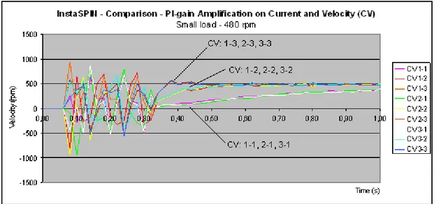
The converted values for InstaSPIN were set by different amplifications in the GUI and the motor was tested on the performance of the step response. The result of the step responses at 480 rpm with the different amplifications of PI-gain in velocity and current can be seen in figure 9. The rise times was

measured from the time were it was started, 0.08 s to the time were the value was at 70 % of its demand velocity and are presented in table 3.

The amplifications were the PI-gain for the velocity regulator are twice the size, CV 1-2, 2-2 and 3-2 the step responses did not overshoot and kept a similar rise time, 0.32 s from 0 to 70% of the demand velocity. However at the amplifications of 3 on the velocity regulator the rise time was 0.27 s which is an improvement but it does overshoot.

At this velocity, a clear pattern of the step responses can be noticed. The pattern shows that an increase on the PI-gain values in velocity regulator shortens the rise time and that the amplification on the current regulator does not significantly

Figure 9: Graph of step responses at 480 rpm using a small load

At the velocity of 1020 rpm an amplification of 3 on the current PI-regulator did not function, therefore neither the step responses nor the rise times are presented at that amplification. As seen in the figure 10 all the step responses will eventually overshoot at 1020 rpm. The setting CV 2-2 have a rise time of 0.26 s and does not overshoot as much compared to the other step responses.

The pattern that was found at 480 rpm is similar at 1020 rpm but the amplification of the current PI-regulator now affects the step response. The effects were for instance shortened rise time and reduced overshoot for some parameters. As seen in the graph the green and pink line are similar, this may be because the

mentioned lines share the same parameters which means that the pink or green line is incorrect and the result of CV 1-3 missing. Due to the missing of a test result, CV 1-3 can not be compared to the CV 2-3. This will create an uncertainty if the overshoot will be reduced at the parameter CV 2-3 therefore it can not be said to be reduced at all parameters.

InstaSPIN - Comparison - PI-gain amplification on Current and Velocity (CV)

Small load - 1020 rpm -1500 -1000 -500 0 500 1000 1500 2000 2500 0,00 0,25 0,50 0,75 1,00 1,25 1,50 1,75 2,00 Time (s) V e lo ci ty (r p m ) CV 1-1 CV 1-2 CV 1-3 CV 2-1 CV 2-2 CV 2-3 Demand

Table 3: The rise times from 0 to 70 % of the demand value at 480 and 1020 rpm

4.1.3 Comparison of PI-gain amplifications at 1500 and 1980 rpm

At 1500 rpm, the amplification of 3 on the current regulator is not functioning and all the step responses overshoot. As shown in figure 11, additional parameters and duplicates were added in order to get a wider view of the consequences when changing the parameters to a larger range. At this velocity the same patterns as from the previous graphs can be seen. A look at the red, blue, green and dark green lines resembles the pattern that shows that increased PI-gain for the velocity regulator reduces the rising time. By comparing the amplification of 1 and 2 on the current PI-regulator, the same differences as in 1020 rpm can be seen. In this case all the rise times are reduced and only the CV 2-1 shows a reduced

overshoot. The patterns can also be noticed in table 4, were the rise times of 1500 and 1980 rpm are presented.

Figure 11: Graph of step responses at 1500 rpm using a small load

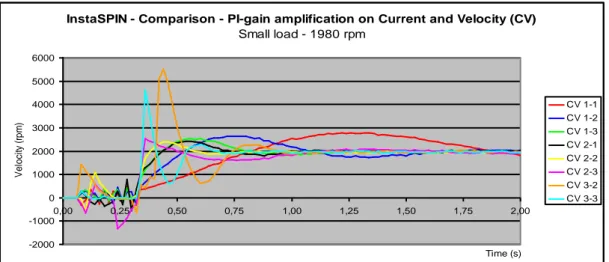
At 1980 rpm the different values react in the same way as both of the known patterns that were discovered which can be seen in figure 12. The amplification 3-1 was found to be not functioning at 3-1980 rpm and therefore excluded from the

InstaSPIN - Comparison - PI-gain amplification on Current and Velocity (CV)

Small load - 1500 rpm -1500 -1000 -500 0 500 1000 1500 2000 2500 3000 0,00 0,25 0,50 0,75 1,00 1,25 1,50 1,75 2,00 Time (s) V e lo ci ty (r p m ) CV 1-1 CV 1-2 CV 1-3 CV 2-1 CV 2-3 CV 2-2 CV 1-0.5 CV 1-1 CV 1-2 CV 1-4 CV 1-6 Demand

Figure 12: Graph of step responses at 1980 rpm using a small load

Table 4: The rise times from 0 to 70 % of the demand value at 1500 and 1980 rpm

In the results of the test phase of PI values, patterns in the step responses can be noticed. It shows for instance that an increase of the amplification on PI-gain values in the velocity regulator will shorten the rise time to a point where the motor eventually stops working. At lower velocities such as 480 rpm the amplifications in the current regulator does not significantly affect the step response. However, at higher velocities the amplification does shorten the rise time and in some cases reduces the overshoot.

The final results of the experiments performed by Saab and the drawn conclusions are shown in table 5. The new chosen PI values were used in all the further test phases.

InstaSPIN - Comparison - PI-gain amplification on Current and Velocity (CV)

Small load - 1980 rpm -2000 -1000 0 1000 2000 3000 4000 5000 6000 0,00 0,25 0,50 0,75 1,00 1,25 1,50 1,75 2,00 Time (s) V e lo ci ty (r p m ) CV 1-1 CV 1-2 CV 1-3 CV 2-1 CV 2-2 CV 2-3 CV 3-2 CV 3-3

4.2 Test Phase - Startup Control

The purpose of this test phase was to understand the use of the parameters in the Startup Control and if changes may have any effects on the startup sequence. The parameters which were changed during the test phase includes: SRT, SC, RSS and RES.

4.2.1 Comparison of the Start Ramp Time

The result of testing the SRT parameter are shown in figure 13, in this case the step response starts at 0,1 s. A distinct difference is seen as the SRT set to the minimum value significantly reduce the ripple by length. The length of the ripple when SRT is set to 1 ms is 0.32 s compared to 1000 ms were it is 1.08 s.

Figure 13: Comparison of SRT value between 1 ms and 1000 ms

From the results a conclusion can be drawn, that the lower the SRT value is, the shorter will the length of the ripple be. Therefore it can be said that the SRT value does affect the startup sequence. The SRT value was set to 1 ms for a minimum ripple.

4.2.2 Comparison of the Startup Current

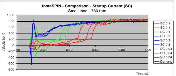
In figure 14, there is a clear difference between the values of SC, apart from one of the green lines that deviates from the other green lines. The blue lines have shorter rise times compared to the other lines. However, the results show a minimal difference in the settling time between the values.

A pattern can be seen, it can be described as that there is a short ripple in the beginning. It either starts negative and then turns positive in velocity or starts

InstaSPIN - Comparison - Start Ramp Time (SRT)

Small load - 1020 rpm -500 0 500 1000 1500 2000 0,00 0,20 0,40 0,60 0,80 1,00 1,20 1,40 Time (s) V e lo c it y ( rp m ) SRT - 1000 ms SRT - 1 ms

Figure 14: Graph showing the comparison of the Startup Current parameters at 780 rpm.

At 1020 rpm, the blue and green lines have rise times that are similar to each other while the red differs as shown in figure 15. While the rise times differs the settling times remains similar. The blue lines maintain its heavy ripple in the beginning as the other lines presents a slightly reduced ripple. At this velocity the said pattern at 780 rpm can be seen but not as clear due to the reduced dead time.

Figure 15: Graph showing the comparison of the Startup Current parameters at 1020 rpm

In both of the velocities a pattern was found and can be described as a ripple in the beginning followed by a dead time and then a rise to the demanded value. We believe that the ripple is the first part of the startup sequence where the solution tries to locate the position of the rotor by energising one of the coils and generate BEMF. As for the dead time it is believed to be the commutation phase where it has to successfully commutate to ensure that it is spinning in the right direction.

InstaSPIN - Comparison - Startup Current (SC)

Small load - 780 rpm -800 -600 -400 -200 0 200 400 600 800 1000 0,00 0,20 0,40 0,60 0,80 1,00 Time (s) V e lo c ity ( rp m ) SC 0.1 SC 0.1 SC 0.1 SC 0.2 SC 0.2 SC 0.2 SC 0.04 SC 0.04 SC 0.04 Demand

InstaSPIN - Comparison - Startup Current (SC)

Small load - 1020 rpm -600 -400 -200 0 200 400 600 800 1000 1200 0,00 0,10 0,20 0,30 0,40 0,50 0,60 0,70 0,80 0,90 1,00 Time (s) V e lo c it y ( rp m ) SC 0,1 SC 0,1 SC 0,1 SC 0,2 SC 0,2 SC 0,2 SC 0,04 SC 0,04 SC 0,04 Demand

From the results, conclusions can be drawn that the higher the SC the shorter the rise time to a point where it gets unstable. It can be said that there is only a

minimal effect on the settling time on any changes on the parameter. Therefore the SC parameter was set to 0.1 to avoid an unstable system.

4.2.3 Comparison of combinations of RSS and RES

A complete result of different combinations can be found in the appendix 2 as only a part of the combinations will be presented in this subchapter.

In figure 16, the step responses of the different combinations can be seen as 2 lines of each combination, starting at 0.1 s. A look on the rise times shows the combinations RSS-RES 100-200, 250-300 and 450-500 has a similar rise time of 0.18 s.

A study of the different values shows a pattern similar to the one found in the analysis of the startup current. A look at the 450-500 value shows the acclaimed pattern, with a negative and positive ripple followed by a constant velocity until an increase of velocity to its demand value. The length of the ripple together with the dead time where the velocity remains constant differs for the different

combinations. For the RSS-RES combinations 50-100, 300-400, 350- 400 the ripple and dead time continues for more than 0.2 s while the other combinations ripple and dead time is shorter than 0.2 s.

Figure 16: The difference between the various combinations of RSS and RES at 780 rpm

At a higher velocity, the dead time together with the ripple are shortened in some cases. A shorter dead time compared to 780 rpm is clearly visible for light blue lines representing 450-500.

InstaSPIN - Comparison - Ramp Start Speed (RSS) and Ramp End Speed (RES)

Small load - 780 rpm -600 -400 -200 0 200 400 600 800 1000 0,10 0,15 0,20 0,25 0,30 0,35 0,40 0,45 0,50 Time (s) V e lo ci ty (r p m ) 50-100 100-200 200-300 250-300 300-400 350-400 400-500 450-500

Figure 17: The difference between the various combinations of RSS and RES at 1020 rpm

From the analysis, conclusions can be drawn that the change of RSS and RES does affect the startup sequence. The effects includes, rise time, ripple and dead time.

4.3 Test Phase - Reliability

When determining the lowest velocity at the startup it came down to understand which combination of RSS and RES worked and if there was some kind of pattern to the working values for each velocity.

Testing for the lowest possible values on RSS and RES for the lowest velocity was done at two different times. The first test phase was done a few days before the second test phase, the second test was needed when the values from the first test did not work later on. The tests from the first test phase are not included in the results and can be seen in appendix 3. The combinations were rated in four categories which can be seen in table 6.

Table 6: Table showing how the fail rate was rated

The velocity of 360 rpm with a small load was the lowest velocity were fail rate of the some tests were higher than 50 %, there were not any combination that made into the good category as seen in table 7.

InstaSPIN - Comparison - Ramp Start Speed (RSS) and Ramp End Speed (RES)

Small load - 1020 rpm -600 -400 -200 0 200 400 600 800 1000 1200 0,10 0,15 0,20 0,25 0,30 0,35 0,40 0,45 0,50 Time (s) V e lo ci ty (r p m ) 50-100 100-200 200-300 250-300 300-400 350-400 400-500 450-500

Table 7: The reliability at 360 rpm with a small load

At 420 rpm with small load there were 14 different setups qualifying for the green category, none for the yellow and three for the red shown in figure 8. All

combinations with RSS set to 35 were in the green category, as well as all the RES combinations up to 210.

Table 8: The reliability at 420 rpm with a small load

At 1200 rpm with heavy load the first setup values with a fail rate of 10 %

appears. With only one good, nine decent setups and the rest poor or worse seen in table 9 less than half of tests was higher than fail rate 50 %. Further tests were done at a higher velocity to find a table with higher account of good and decent values.

Table 10: The reliability at 1260 rpm with a heavy load

When increasing the velocities the number of combinations with good fail rate increases and the does not function category decreases. Thus increase in velocity increases the overall combinations that qualify for poor or higher categories increase. Another pattern can be seen but only at the results of when a small load was used. It can be described with the combinations performs relatively better with a RSS value that is half of the demanded velocity.

From the results, the velocities, 420 and 1260 rpm were chosen as the lowest stable velocities because of several categories were rated good which can be compared.

4.4 Test Phase - Optimal Step Response

The purpose of these tests were to find the most optimal RSS and RES values for the lowest velocities that was decided, 420 and 1260 rpm. In this subchapter the results of the first run presented as the results for the second run can be found in the appendix 7.2.

The step responses were started at 0.1 s and recorded to 1 s, as seen in figure 18. At 420 rpm the combinations differ and the same pattern described in the subchapter 4.2.2 can be seen.

Figure 18: Comparison from the first run between the different step responses at 420 rpm with a small load

At 1260 rpm most of the step responses have the same distinct pattern at the lower velocity, 420 rpm. There is a noticeable difference between the step responses as some combinations which perform better than others.

Figure 19: Comparison from the first run between the different step responses at 1260 rpm with a heavy load

From a study of the graphs including the two from the second run, the optimal combination was set to 70-210 for 420 rpm respective 315-840 for 1260 rpm. The final results from the optimisation of InstaSPIN and the finding of the lowest

InstaSPIN - Comparison RSS/RES

Small load - 420 RPM -600 -400 -200 0 200 400 600 800 0,00 0,10 0,20 0,30 0,40 0,50 0,60 0,70 0,80 0,90 1,00 Time (s) V e lo ci ty (r p m ) 35-70 35-140 35-210 35-280 35-350 35-420 35-490 70-140 70-210 105-140 105-210 140-210 175-210

InstaSPIN - Comparison RSS/RES

Heavy load - 1260 RPM -1000 -500 0 500 1000 1500 0,00 0,10 0,20 0,30 0,40 0,50 0,60 0,70 0,80 0,90 1,00 Time (s) V e lo ci ty (r p m ) _105-1050 210-1260 210-1470 315-840 420-840 525-840

Table 11: The lowest stable velocities for small and heavy load together with the optimised parameters.

4.5 Test phase - Step response and distance

What is the performance on the startup sequence in the matter of rise time and settling time from zero to lowest stable velocity?

The purpose of the test was to see how the motor rotates during the startup sequence with InstaSPIN compared to EPOS2 and how many revolutions the systems accomplish until a set time. As it is presented in figure 20 EPOS2 has quicker step response than InstaSPIN. The rise time which measured from stationary to 70 % of its final value was 0.61 s for InstaSPIN. As for EPOS2 which can not be determined as precisely as InstaSPIN because of the resolution is too low but is less than 0.01 s.

The settling time which is the time taken for the system from a stationary velocity to be in the range of ±5 % of its final value. For InstaSPIN it took about 0.97 s before it is in the 5 % interval respective 0.09 s for EPOS2. The difference of 0.88 s means that EPOS2 was more than 10 times faster than InstaSPIN at settling time. In this case the settling time is measured from a stationary velocity but with the ripple and the dead time excluded the settling time of InstaSPIN would be 0.53 s which is only 6 times slower than EPOS2. The rise time without ripple and dead time would be 0.17 s.

In the figure a pattern can be seen, it shows a dead time between 0.2 s and 0.4 s where it does not increase in velocity when it should. This pattern resembles those seen the startup current test phase. This may be improved by increasing the

startup current but increased startup current will probably increase the commutation pattern in the beginning.

Figure 20: The step response of InstaSPIN and EPOS2 from 0 to 420 rpm with a small load.

The difference at the startup sequence is for instance that EPOS2 goes further in distance under this short time as seen in figure 21. For InstaSPIN even with the entire ripple in the beginning it does steadily move forward without stopping. The difference under this test comes down to the difference in revolutions for the systems. EPOS2 ends at 9.4 revolutions and InstaSPIN ends at 7.3 revolutions.

Figure 21: The revolutions during the step response for InstaSPIN and EPOS2 at 420 rpm

Looking closer at the beginning in distance there is no greater impact of the ripple in distance, speed is just a bit lower during this short moment as shown in figure 22.

Step Response Comparison

Small load - 420 rpm 0 100 200 300 400 500 0,00 0,25 0,50 0,75 1,00 1,25 1,50 Time (s) V e lo c it y ( rp m ) InstaSPIN EPOS2 Demand Distance Small load - 420 rpm 0 2 4 6 8 10 0,00 0,25 0,50 0,75 1,00 1,25 1,50 Time (s) Revo lutio ns InstaSPIN EPOS2