The influence of real estate price fluctuations on real estate stocks : An analysis of Swedish asset classes

(1)

The influence of real estate price

fluctuations on real estate stocks

An analysis of Swedish asset classes

BACHELOR THESIS WITHIN: Economics NUMBER OF CREDITS: 15

PROGRAMME OF STUDY: International Economics AUTHOR: Jesper Jonasson & Tobias Rosén

(2)

Acknowledgements

We, Jesper and Tobias, would like to thank the persons who have contributed with feedback and constructive criticism in our process of writing this thesis.

Foremost a big thank you to our mentor, Dr. Michael Olsson, who has provided support and words of advice, always with a smile on his face.

We would also like to acknowledge our seminar group members who have devoted their time in order contribute with sound opposition.

_______________________________ ________________________________

Jesper Jonasson Tobias Rosén

Jönköping International Business School May, 2019

(3)

Bachelor Thesis within Economics

Title: The influence of real estate price fluctuations on real estate stocks Authors: Jesper Jonasson and Tobias Rosén

Tutor: Michael Olsson Date: 2019-05-28

Key terms: Real estate, Real estate stocks, Stock market, Supply and Demand, Interest rate, Capital Asset Pricing Model

Abstract

With background to recent price growth in Swedish real estate and consequently real estate stocks, our aim is to examine the relationship between real estate price development and real estate stock price development. To test our hypothesis, that real estate price development have had an impact on the return of real estate stocks, we built a capital asset pricing model. We divide the return of real estate stocks into two parts, the return in relation to the Swedish market premium and the excess return that is given for the exposure of the real estate market. We found that real estate exposure would treat the investor with an additional return beyond the return given from stock market exposure; hence, real estate price development has contributed to real estate stock returns.

(4)

1. Introduction

Factors such as the interest rate, supply and demand, play an important role in the dynamics of asset pricing. According to data from Statistics Sweden (SCB, 2019a), the average citizen in Sweden holds two types of economic assets, real assets and financial assets. Real assets are physical assets, which are tangible objects that have a value due to the object itself and not naturally due to the operation of the object, such as real estate. Financial assets do not necessarily have a physical value; financial assets rather yield a return due to a contractual claim, like stocks or bonds. This thesis will treat real assets as real estate, and financial assets as stocks, as these two are the most accessible for an investor. Understanding the price dynamics in both of these assets and the relationship between them are of importance to investors as these assets often sum up to a large part of a household’s balance sheet. Looking historically in Sweden, a real estate investment has yielded lower annualized returns than stocks, but looking at recent data, we can see that real estate and especially real estate stocks have outperformed the broad stock indices in Sweden (Edvinsson, et al., 2014). So far, the majority of the research completed in this area has focused on the real estate market and its performance, but with this thesis, we aim to add to an explanation for why the real estate stocks have been outperforming the market.

To be able to conduct this investigation we needed to look at how each of the asset classes were valued and understand the link between them. The valuation of an asset is reflected in the price of that specific asset, the price of the asset is determined by supply and demand (Rittenberg, et al., 2016). In general, terms, the microeconomic law of supply and demand will reflect the assets price and beyond this, the price can often be explained by macroeconomic theory that suggests that low interest rates will stimulate an economy in such that the price of assets will increase (Gärtner, 2016).

The supply of real estate assets is the total amount of real estate in Sweden, though only the vacant real estate is the supply buyers will observe. Regulations by the government have a large impact on the amount of real estate produced since the suppliers must follow these guidelines (Boverket, 2019a). If the supply of real estate is scarce and demand is high, by the law of supply and demand, the price should increase. When it comes to supply

(6)

and demand in financial assets such as stocks and bonds, they as well follow the same microeconomic theory. A stock is traded on a stock market, the demand for the stock depends on the amount of buyers and the average quantity they wish to purchase, and the supply of the stock depends on the amount of sellers and the average quantity they are willing to sell. When a stock is faced with a surplus of buyers versus sellers, we will observe an increase in stock price (Berk and DeMarzo, 2017).

There are two ways to be exposed towards real estate assets. The first option is to purchase the real estate as a physical asset, that is, an actual physical real estate such as a house, apartment or warehouse. The second option to get exposure towards real estate without purchasing the physical asset is to by real estate stocks. That is, to invest in companies that have a portfolio of real estates of various kinds. Exposure to these two real estate assets will face the economic agent with the same fundamental asset but with different characteristics. For example, real estate as a physical asset could be bought for other reasons than the opportunity of future earnings, as the real estate stock would be bought for. These different characteristics will differentiate the demand and supply of each asset, causing a unique price dynamic for each asset. This is because even though they do face the same prevailing economic environment, which will impact asset prices (Quan and Titman, 1999), each asset faces unique incentives in the decision of purchase.

The purpose with this thesis is to investigate if and by how much Swedish real estate prices affect the real estate stocks traded on the Stockholm stock exchange. Real estate as a physical asset and financial asset are both assets with the same underlying resource but faced with different demands and supplies due to the characteristics of the asset classes. A house or a warehouse is not often bought for the expectation of future earnings, but for the benefit it yields in terms of functionality. The difference in characteristics provide us with the question whether we can determine the origin of the return in real estate stocks. We have chosen to look at the period 2005-2017, mainly because this covers an entire business cycle and most importantly, it covers the time real estate as an asset started to outperform the market. We will test the effect of real estate prices by setting up a model in which we can isolate the returns of real estate stocks due to market movements, that is the risk they are faced with, and isolate the excess return given by the growth of real estate prices.

(7)

With help from our model, we found that the real estate stocks are faced with a higher risk than the market and accordingly they will have greater movements, in both positive and negative directions. We also found a significant excess return explained by real estate price increases.

The thesis will be organized in the following way. Chapter one provides the introduction and chapter two introduces the reader to the theory and a hypothesis. Chapter three presents the data and chapter four the method. Chapter five display our empirical results and analysis. Chapter six will conclude the thesis with a conclusion.

2. Theory

Quan and Titman (1999) conducted an international investigation if real estate prices moved together with stock prices. The background for their research was due to that a number of authors had argued for real estate offering diversification to investors because of the low correlation to broad stock indices. For example, Eichholtz and Hartzell (1996) found surprisingly low correlation between stock indices and real estate indices in mature economies such as in the U.K, U.S and Canada. What made Quan and Titmans research unique is the fact that they were able to find a significant correlation between real estate prices and broad stock indices; this was conflicting with previous research. According to their report, they describe the correlation as this;

“The correlation between stock returns and real estate price changes will arise if business cycle variables simultaneously affect corporate profits and rents. In addition, stock and real estate prices will also move together if expectations (either rational or irrational) about future profits and rent move together” (Quan and Titman, 1999, p. 205). In summary, the major part of the correlation can be explained by economic fundamentals that simultaneously influence real estate and stocks (Quan and Titman, 1999).

2.1 Assets and monetary policy

Real estate assets such as houses and apartments are most often the largest asset in a household. It is important to understand the price dynamics of these real estate assets as

(8)

the fluctuations in house prices will influence the economic business cycle. Thus, knowledge on dynamics in real estate prices is key for central banks in their monetary policy decision making which consequently will influence the national economy such as disposable income and development of stock indices. (Tsatsaronis and Zhu, 2004). The importance of real estate prices has led to extensive research on real estate markets but less on the integrated underlying asset, real estate traded on a stock market.

One major tool to regulate asset prices is the use of monetary policy; in this case, it is the interest rate. A decrease (increase) in the interest rate will lead to an increase (decrease) in prices and demand of assets. The reason people and businesses invest their money is for the opportunity of future earnings, hence the tool used to invest is money. When interest rates decline, the cost of money is decreased as you can borrow inexpensively. This will stimulate demand for assets as firms and persons will be able to foresee investment opportunities cheaper. All else equal, an increase in demand will lead to increased prices according to the law of demand. The supply of assets is determined by the money supply, as investments are limited to the accessible money in a market. The supply of money is determined by the central bank in a country and is often set to a fixed level in economic theory. When money supply is increased (decreased) we will observe a lower (higher) interest rate that will in line with previous explanation of investment demand, increase the demand of money, hence investments (Shiller, 2008).

2.2 Supply and demand in the Swedish housing market

To understand the supply side of real estate helps investors realize how much prices might fluctuate in the future. The supply of real estate assets can be explained by the amount built by different suppliers. There are limitations when it comes to supply and demand in the housing market. Legislations have a large impact on the amount of real estate produced since the suppliers must follow these guidelines (Boverket, 2019a). Such as, on the supply side, it is limitations in land supply and restrictions on how much that is allowed to be built that determines the supply of real estate (Shiller, 2007). If the supply increases, the price should by microeconomic law of supply and demand decrease. Demand in real estate can be interpreted as a function of the population (Mulder, 2006). The population in Sweden is growing by approximately 0.83 percent per year (Sweden Population, 2019). The population in Sweden is mainly growing due to immigration.

(9)

Comparing year 2000 and 2017, the number of people that have immigrated to Sweden has tripled, approximately 50,000 in year 2000 and 150,000 in 2017 (SCB, 2019b). The population in Sweden is continuously growing and this influences the prices of real estate. If the population in Sweden grows faster than the supply of residential housing the market will face an excess demand of real estate. Excess demand will act as a driver for prices; hence, the prices should increase (Thedéen. 2017). If the population growth slows down, the opposite should be true, the supply of real estate should be in excess of demand, and the prices should decrease.

In addition to the population, the income level of the population affects the prices of real estate. The income effect says that if the income in a country increases, the prices of normal goods should in theory increase as the amount of money circulating in the economy increases, thus people have more to spend, increasing their purchasing power (Tsatsaronis and Zhu, 2004). To measure the income level, one can observe the gross domestic product per capita (GDP per capita) which measures the market value of all the final goods and services produced per person in the country. If the GDP per capita increases, we should according to previous theory, exhibit an increase in real estate prices. The same is true in the opposite direction, if the GDP per capita decreases, the real estate prices should decrease.

2.3 Supply and demand in the stock market

A stock is traded on a stock market, the demand for the stock is the amount of stocks the buyers are willing to purchase, and the supply of the stock is the amount of stocks that the sellers are willing to sell. The total supply of a stock consists of the amount of shares that are emitted. Usually there is a limited amount of shares that are issued and therefore there is a limited total supply. If a company generates results that satisfy the investors, by microeconomic law of supply and demand, the price of the stock should increase since buyers demand for the stock will increases due to the positive results.

There are several different approaches when it comes to valuing and finding the fair price of a stock, one major distinction can be made whether the stock is a value stock or a growth stock. A value stock is most commonly labeled by looking at the price-to-book ("/$) ratio of the firm. When a low ratio is observed, we can assume that the market

(10)

values the stock largely due to its book value and not after future earnings prospects. For example, for a firm which has a "/$ of exactly one, the market values the stock to the exact value of the company's book value. The book value of a company is the collected value of all their tangible assets on their balance sheet. Therefore, a value stocks price will be determined to a large degree by the development of their asset values. A growth stock has, in contrast to value stocks, a high "/$, this can be interpreted as that the market does not value the net assets of the firms too highly, but the value rather rests in the expected high growth rate of future earnings (Fama and French, 1998). Real estate stocks in Sweden have a relatively low "/$ ratio thus the price should be affected by the valuation of their underlying assets (Börsdata, 2019).

Both demand and supply are driven by future expected earnings and asset valuation. The demand increases when the expected future returns and asset values are expanding while the supply increases when the expected future returns and asset conditions turn negative, as investors will shift to assets with brighter prospective outlook (Berk and DeMarzo, 2017). There are both sellers and buyers in the stock market due to a difference in opinion between the investors. There are different ways to value companies and different methods provide different results, therefore there are investors at opposite sides, both buyers and sellers. The two groups’ decision mechanisms are driven by general human behavioral aspects and their financial investment decisions are influenced by the macroeconomy and company events (Lind and Lundström, 2009). Future earnings and asset valuation are partly governed by the prevailing macroeconomic conditions; the investor will have a higher demand for stocks when future economic growth looks robust (Levine and Zervos, 1996). The stock market is strongly correlated to the long-run economic growth. By looking at the gross domestic product per capita level, an investor can assume that the stock market will reflect the economic growth of that country (Levine and Zervos, 1996).

2.4 Comparing Supply and Demand within the two markets

The supply and demand in the real estate market and real estate stock market are to a large degree influenced by the same macroeconomic fundamentals, thus we should expect that the price dynamics between the markets should move in equal trends (Quan and Titman, 1999).

(11)

What differentiates the two markets is the motives behind investing in each of them. The sole purpose of investing in a stock, in our case, a real estate stock, is for the economic incentive. A stock is bought for the expected return that the investor will earn through price growth and dividend payouts. The price for the stock is thus determined by the expectations of future earnings that the specific stock will be able to return to the investors. In real estate stocks, these future earnings are established in both the real estate market and the stock market. In the real estate market, as real estate stocks have a low "/$ ratio. The price of the stock should therefore be influenced by the price dynamics in the real estate market, in which real estate stocks hold most of their assets. In the stock market, as real estate stocks have a company behind them operating to earn returns to its shareholders by using its assets to earn rents. A real estate asset can be bought for the same reason as for a stock, to earn a fair return. A real estate asset can also be bought in terms of functionality, serving the investor with utility other than just expected returns. This imposes the demand of real estate with unique characteristics, thus the price of real estate assets should not be solely determined by the prospects of future earnings but rather also be affected by the demand for the functionality that real estate satisfies (Goodman, 2003). Both the stock and real estate market therefore influence real estate stock prices.

2.5 Macroeconomic fundamentals

In this thesis, we have separated the origin of returns for real estate stocks into two separate markets, the real estate market and the stock market. Within these two markets, there are underlying macroeconomic fundamentals, affecting each of the markets supply and demand equilibrium. We will assume that the effect of these underlying factors will be represented in the price points we gather in our data but want to shed some light on how some of the major macroeconomic factors will impact the stock and real estate market.

The interest rate is a factor that influences both the real estate market and the stock market. The interest rate is the rate at which banks can lend or place liquid funds at the Riksbank, the Swedish central bank. The interest rate is used as a tool to control the inflation level in Sweden, hence preserving monetary value (Riksbank.se, 2019). The interest rate is important in both of our markets since a decreasing interest rate will let individuals take advantage of borrowing money cheaply and can therefore foresee their

(12)

investment opportunities easier, both the investments in real estate and in the stock market (McCue and Kling, 1994).

The GDP (Gross Domestic Product) growth rate in Sweden measures how fast the Swedish economy is growing and provides us with basis for if the economy is booming or stagnating. The GDP growth rate is important for both the real estate market and the stock market since when the economy is booming or stagnating the investors demand for investments will shift (McCue and Kling, 1994).

The consumer price index (CPI) measures the price development of a basket of goods and services and is a type of inflation measurement. The inflation rate affects the amount of spending in the economy. If the inflation rate is low, the price of goods is increasing at a slow rate and therefore the value of the money decreases at a slower speed. This will affect individuals urge of spending and investing to decrease, relative to a higher inflation rate. If the inflation rate is higher individuals would prefer to spend their money since their purchasing power is decreasing. Real estate assets, whose prices increase when the inflation rate rises, could therefore be bought to hedge against the holdings in currency since if the inflation rate rises, the currency’s purchasing power decreases, while the real estate asset would increase in value (Case and Wachter, 2011). The interest rate, GDP growth rate and the inflation rate affect the real estate market and the stock market simultaneously while market specific factors, such as the production of real estate which influences the real estate market to a large degree, does not impact the stock market as much. This is why we need to keep the prices of the real estate market and the stock market separate since they exhibit unique supply and demands when modelling for real estate stocks (McCue and Kling, 1994).

2.6 Real estate traded on the stock market

According to the modern portfolio theory (MPT), the goal of an investor is to earn a fair return related to the risk that is being taken (Markowitz, 1952). An investor could purchase real estate stocks or real estate in physical form in order to diversify oneself and create an optimized portfolio. By including real estate stocks or actual real estate in a portfolio already consisting of stocks and other assets, the investor diversifies even more

(13)

and minimizes the firm specific risk due to diversification, and only faces the market-risk (Berk and DeMarzo, 2017).

Sharpe (1964) was one among the initiators of the Capital Asset Pricing Model (CAPM), a model that describes a relationship between expected return and risk when investing in an asset, model (1). The addition in the CAPM compared to the modern portfolio theory is that the CAPM shows a relationship between risk and return but with a risk premium & '( − *+ , explaining the return that the investor requires from the

investment instead of in risk-free assets. An alpha, ,, showing excess return, a beta, -_., explaining the risk relative to the market and an error term, epsilon, 0_., showing the firm specific risk (Sharpe, 1964). The capital asset pricing model is as follows:

&('.) = '++ , + -. &('() − '+ + 0. (1)

Developed version of the capital asset pricing model has been done by Fama and French (2004) where they add the difference in performance between small-cap compared to large-cap companies (SMB, Small Minus Big) and the performance between low price-to-book companies compared to high price-to-market companies (HML, High Minus Low) (Fama and French, 2004). The Fama-French Three Factor Model is as follows:

& '_. − '₊ = , + -₃ &('₍) − '₊ + -₄ 56$ + -₇ 869 + 0_. (2) An idea within the Fama-French Three-Factor Model is to make the variables self-financed. Since the investor sells or shorts one side of the variables HML and SMB and then buys the other side, the investor is able to use the proceeds from the short sale in order to finance the purchase of the other side (Fama and French, 2004).

We also build upon the capital asset pricing model because the model provides variables that help us understand the origin of the return and potential excess return. The CAPM provides the beta term, which symbolizes the amount of risk the portfolio has relative to the market. The model also provides an alpha term, which describes the excess return received relative to the benchmark index and risk. Included in the model is also the risk-free rate, which is deducted from the expected market return, which together are called

(14)

risk premium. The risk premium explains the return that the investor requires in order to hold positions in the market instead of in risk-free assets. Beta in our model will show the amount of risk that the real estate stocks will have compared to the market thus will show variations due to market fluctuations. Investors use the alpha in the CAPM to measure how much excess return their strategy achieves. We will be using the capital asset pricing model because we are looking at how much the real estate prices, RESINDEX, are affecting the real estate stocks, SX8600PI. We are adding the real estate returns variable to the CAPM model since we believe that real estate price development will contribute to excess return in simultaneity with the original alpha, which is unknown. Investing in the stock market and simultaneously in the real estate market involves extra risk-taking and since we have observed that the real estate index has outperformed the market index, the investor should be compensated for that risk by earning an extra return. We are using the expected return for the OMXSPI index since this is the index covering all stocks on the Stockholm Stock Exchange and should therefore represent the Swedish expected return for stocks. The OMXSPI and the real estate stocks (SX8600PI) are also both financial assets and is another reason for why the market index should affect the real estate stock index. Since we are using a real estate stock index, we can assume that the idiosyncratic risk is zero, as the diversification removes the firm specific risk (Berk and DeMarzo, 2017). This gives us model (3).

5:8600"> − '₊= , + -₃'&5>?@&: + -₄ &(A6:5">) − '₊ (3)

2.7 Hypothesis

With support from our theory and our developed capital asset pricing model, we can motivate our following hypotheses:

• We expect an additional risk in the real estate market. -₃ > 0

• We expect that real estate stocks earn the investor an extra return due to the additional risk faced in the real estate market. If alpha together with the additional risk multiplied by the average return in real estate prices is greater than zero, we can confirm that real estate stocks will yield an excess return compared to the market premium: (, + -₃'&5>?@&:) > 0

(15)

Where:

'&5>?@&: = CℎE GHE*GIE JKLCℎMN *ECO*L KP '&5>?@&:

3. Data

To investigate the relationship between Swedish house prices and real estate stocks traded on the Swedish stock market, data for the dependent and explanatory variables are collected over the period 2005-2017. All data is converted from index values to monthly returns. The reason for the chosen time interval is to include data that covers both before and after the financial crisis in 2008.

To calculate the market risk premium and returns adjusted for the risk-free rate, we need to have data for the risk-free rate, RF. This is the ten-year Swedish government bond with a constant maturity rate. It is collected with a constant maturity rate in order to pick up the fluctuation of the rate over our period. The gathered rate is the yearly rate, thus it had to be divided by twelve in order to get the monthly risk-free rate to match our time frequencies in our previous variables. The data is gathered from the Federal Reserve Bank of St. Louis (FRED, 2019a).

The dependent variable, OMX STOCKHOLM REAL ESTATE PI, is a real estate stock index covering all of Stockholm stock markets real estate stocks. The data is gathered on a monthly basis and is the average price of each month (NASDAQ, 2019a). In our regression, this variable is SX8600PI and SX86_RF, where the latter one is adjusted for the risk-free rate.

The first independent variable is a residential real estate price index, denoted RESINDEX and RES_IND_RF, where the latter one is adjusted for the risk-free rate. The data is collected on a quarterly basis (FRED, 2019b), thus needs to be converted into monthly in order to match the current time frequency in the model. The conversion was completed by using Eviews and the tool quadratic match, which estimates the missing monthly values. We assume that this index represents the overall development of real estate prices in Sweden and we will therefore not include a real estate index covering non-residential real estate.

(16)

The second independent variable is OMXSPI and OMXSPI_RF, where the latter one is adjusted for the risk-free rate. OMXSPI is a stock index covering all the stocks traded on the Stockholm stock exchange. This represents the overall development of the stock market in Sweden and can be interpreted as the market risk premium. The data is gathered in the same manner as the real estate stock index, SX8600PI (Nasdaq, 2019b).

3.1 Descriptive statistics

We have 157 observations as we collected the monthly data over 13 years for all our variables. The number 157 arise due to the nature of calculating returns, when one calculates returns the succeeding months value is needed to calculate the return for current month, hence the first month of 2018 is observed to get the return for the last month in 2017. From the tables below we can observe that our largest monthly return, 25.18 percent, is found in our real estate stock index, real estate stocks also yield the highest average return. We can also observe that the standard deviation is the highest in this variable. The lowest return in our sample is found in the broad stock index, OMXPI, at -19.71%. Residential house price returns have the lowest average return but also the lowest standard deviation. In the risk-free rate, we can see substantial fluctuations over time as the smallest value versus the largest differ a lot. The variables, in which the risk-free rate is subtracted, are logically smaller by roughly the average risk-free rate.

Table 1.

Variables Obs. Mean Std. Dev. Min Max

SX8600PI 157 0.86% 6.20% -17.09% 25.18% OMXSPI 157 0.58% 4.72% -19.71% 17.17% RESINDEX 157 0.53% 0.76% -3.62% 2.70% SX86_RF 157 0.61% 6.21% -17.38% 24.97% OMXSPI_RF 157 0.33% 4.73% -20.02% 16.92% RES_IND_RF 157 0.28% 0.76% -3.92% 2.32% RF 157 0.25% 0.09% 0.13% 0.43%

(17)

4. Method

The data for our variables was gathered as indices with data points for each month. To create normalization in our indices we will use the natural logarithm, this will let us analyze the returns of the indices even though we have unequal starting values. The return for an index i and time t is then calculated as in the following equation:

*ECO*L. RLSET_.,U = ln RLSET_{., UX3} − ln (RLSET_.,U) (4) We then had to reduce the returns of the indices by the risk-free rate. As the risk-free rate data was gathered as monthly rates we did not have to carry out any transformation for this variable. We calculated the risk-free adjusted return for index i at time t, as in the following equation:

GSY. *ECO*L. RLSET.,U = ln RLSET., UX3 − ln RLSET.,U − '+,U (5)

Our estimated model builds upon the capital asset pricing model as stated above in model (1). In our thesis, we are using the real estate stock index returns SX8600PI as our dependent variable and we use residential real estate returns, RESINDEX, as an explanatory variable together with the expected market return, OMXSPI. As our hypothesis states, we believe that the real estate returns are the reason for the performance in the real estate stock index SX8600PI and we will therefore add the real estate prices variable RESINDEX into the model we call “CAPM with RESINDEX”:

5:8600"> − '₊= , + -₃'&5>?@&: + -₄ &(A6:5">) − '₊ (3) Where: 5:8600"R = *EGM EZCGCE ZCK[\ *ECO*LZ '₊= *RZ\ − P*EE *GCE , = GM]ℎG '&5>?@&: = *EGM EZCGCE *ECO*LZ A6:5"> = JG*\EC *ECO*LZ

(18)

We will also test two alternative models, which for one we do not deduct the risk-free rate from the model (3) which we called “CAPM with RESINDEX”, as seen in model (6) which we will call “CAPM with RESINDEX and no free”, and one where the risk-free rate is deducted from the entire model, including our real estate index, model (7) which we will call “CAPM with risk-free adjusted RESINDEX”.

5:8600"> = , + -₃'EZRLSET + -₄ &(A6:5">) (6) 5:8600"> − '₊ = , + -₃ 'EZRLSET − '₊ + -₄ & A6:5"> − '₊ (7)

4.1 Stationarity

Due to the fact that we have time series data we need to investigate if our variables are stationary in order to be able to conduct an ordinary least square (OLS) regression. Our variables were tested with an augmented Dickey-Fuller unit root test. If the results display integrated times series of order I(d) and d > 0, hence they are non-stationary, we should in theory take the difference until we find I(0), but before doing that we controlled for cointegration. Cointegration is the phenomenon when times series share a long run common trend and the residuals are stationary, resulting in the removal of the stochastic trend that is naturally present in non-stationary time series. Cointegration allow us to estimate our regression with an ordinary least square regression even though if non-stationarity is found in our variables (Gujarati & Porter, 2010). We performed a Johansen cointegration test, it utilizes a vector autoregressive model (VAR) and permits the testing of more than one cointegrating relationships. The Johansen test allows all of the variables in the regression to be used as dependent variables, maintaining the cointegration result. The test will tell if there is none or at most one cointegration vector, indicating the direction of stationarity. The null hypothesis for the Johansen cointegration test is that there is no cointegration (Cheng, 1999).

4.2 Multicollinearity

To ensure efficiency in our regression we set up a test for multicollinearity. Multicollinearity is the problem of highly correlated explanatory variables in a multiple regression model. When multicollinearity is present, a number of issues can skew the estimates of the model, e.g. standard errors are too high and the relevance of the

(19)

explanatory variables effectiveness on the dependent variable is uninteresting due to correlation among the explanatory variables. We tested for multicollinearity by applying the variance inflation factor (VIF) together with the assumption: centered VIF > 10 interpreted as severe multicollinearity (Gujarati & Porter, 2010).

4.3 Heteroscedasticity and autocorrelation

Heteroscedasticity is an issue when running ordinary least square regressions as it terminates the assumption of constant variance in error terms; instead, error terms are not constant and change systematically. We tested for heteroscedasticity by applying the White test. Positive autocorrelation is the problem of the error terms being correlated and thus violating the OLS assumption that error covariance is zero. We tested for autocorrelation with Durbin-Watson statistics. A remedy to fix these problems is to apply the heteroscedasticity and autocorrelation corrected (HAC) Newey-West estimation method. This does not alter our estimation but only corrects the standard errors to solve the problem of autocorrelation and heteroscedasticity (Gujarati & Porter, 2010).

5. Empirical Results and Analysis

This chapter will provide a description of the results from our robustness tests and tested models and as well as an analysis of the results.

5.1 Stationarity tests

The augmented Dickey-Fuller tests conducted on our variables indicated that a unit root was present in all our variables, hence we have non-stationarity. This leads us to the results from our Johansen cointegration tests. These results confirm that we can reject the null hypothesis, that we have no cointegration at five percent significance level. These results provide us with support of running our OLS regression with non-stationary variables and the results are visible in appendix A.

5.2 Multicollinearity, Heteroscedasticity and Autocorrelation

Regarding our tests for multicollinearity, we found centered VIF < 10. Our centered VIF values were around 2.5 thus we have not found support for multicollinearity in our multiple regression model, as seen in table 2 below. We tested for heteroscedasticity by applying the White test and could reject the null hypothesis that we have homoscedasticity

(20)

present, interpreted that heteroscedasticity is present in our data, this is also seen in table 2. We found positive autocorrelation in the estimated model from OLS as we had a Durbin-Watson test statistic between 0 and < 2, indicating strong positive autocorrelation, displayed in table 2. As both heteroscedasticity and autocorrelation were present, a suitable solution was to apply HAC Newey-West estimation method. In table 3, when HAC Newey-West estimation was applied, we saw no difference in the estimations, as anticipated, only in the standard errors. This could impair our probabilities but it did not. It can be noted that the above holds for all the three models we tested.

Table 2. Variance inflation factor tests for multicollinearity, White test for heteroscedasticity and Durbin-Watson statistics for testing autocorrelation for all models. Efficiency tests 2005 - 2017 Centered VIF Obs*^ _ _Durbin- Watson N Model 3 1.5805 43.4207 (0.0000) 0.2288 157 Model 6 3.5948 46.2431 (0.0000) 0.2200 157 Model 7 2.0655 32.6571 (0.0000) 0.2379 157

Note: Centered VIF < 10 indicates no multicollinearity. Obs*'4_{is the Breusch-Godfrey}

LM test statistics and the parenthesis display the chi-square probability, at 1 percent significance level we can reject the null hypothesis that we have homoscedasticity. Durbin-Watson displays a measure for autocorrelation, the range between 0 to < 2 indicate positive autocorrelation. N informs about the sample size.

5.3 Results

With our developed version of capital asset pricing model, CAPM with RESINEX, we found our, -₃, the coefficient that measures the return given from the risk taken in the real estate market, to be positive. The alpha in this model is negative. We cannot reject our first hypothesis, -3 > 0. We cannot reject our second hypothesis , + -3'&5>?@&: >

0, this is because the average monthly return in the real estate market, seen in table 1, is 0.53% over our observed period. That together with the positive -₃ will outweigh the negative alpha. This version of the CAPM can confirm that over our chosen time period,

(21)

investing in real estate stocks yielded excess return compared to the stock market. We got the result that real estate stocks have higher risk than the stock market in Sweden as we found -₄ > 1. This signals that real estate stocks will face higher volatility compared to the market. The results are viewable in table 3 under model (3).

In our second tested model, CAPM with RESINDEX and no risk-free, where we did not deduct the risk-free rate from any variables, we found a somewhat smaller effect from the real estate returns and a modest difference in the volatility to the stock market.

In our last model, CAPM with risk-free adjusted RESINDEX, with the risk-free rate deducted from the entire model including residential house price returns, we could observe a substantial change in our volatility compared to the market as our -₄ approaches one. The real estate returns in this versioncontributes to a larger reaction in real estate stocks than in previous models. The risk, measured in the beta coefficients, is larger in the real estate market than in the stock market in this model as -₃ > -₄. We also find that our alpha is larger and together with the increase in -₃ we find a larger excess return compared to the risk taken in the stock market. We cannot reject any of our two hypotheses for this version of the CAPM. The results for all models are displayed in Appendix A, and in table 3 with HAC Newey-West standard errors.

(22)

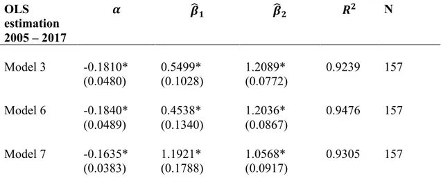
Table 3. Ordinary least square estimations with HAC Newey-West corrected standard errors OLS estimation 2005 – 2017 a b_c b_{_} ^_ _N Model 3 -0.1810* (0.0480) 0.5499* (0.1028) 1.2089* (0.0772) 0.9239 157 Model 6 -0.1840* (0.0489) 0.4538* (0.1340) 1.2036* (0.0867) 0.9476 157 Model 7 -0.1635* (0.0383) 1.1921* (0.1788) 1.0568* (0.0917) 0.9305 157

Note: The estimates above are obtained from the least square regression of equation 3, 6 and 7, The values in parentheses denotes the Newey and West standard errors. *, indicate the 1 percent significance level for when we can reject the null hypothesis, - = 0. The sample period is 2005M01 to 20018M01. 4is the coefficient of determination, which explain to which degree independent variables explain variance in the dependent, 1= full explanation. N displays the number of observation for each regression.

5.4 Discussion

In the CAPM with RESINDEX, we found the estimated volatility of real estate stocks to be larger than the one faced in the stock market. This translates to that real estate stocks face higher risk than the stock market in general, thus investors should be compensated for this extra risk. Real estate stocks are in general value stocks as they are priced to low "/$ ratios, which implies that the asset value contributes to a significant part of their stock price. However, the asset value is only a part of the entire valuation; the second part of the valuation should be the due to future earnings prospects. Real estate firms earn their operating returns by rents and increasing values of their assets that later can be sold for profits. Rents tend to increase when the real estate prices increase, (Plazzi, et al., 2010), thus earnings will increase in two instances when the real estate market booms. We assume that this leverage will increase the volatility of the earnings for real estate companies. People can also, somewhat effortless, shift the object they rent, resulting in uncertainty in earnings from rents. Additionally, with recent price development in real estate, which has been steep and fast relative to historical standards, we can therefore speculate that additional risk in real estate stocks must exist.

(23)

We can together with our tested models and results confirm that we will see an additional return given due to the extra risk faced in the real estate market. This additional return is less than if we would have invested directly into the real estate market, as the relative volatility, -₃ is lower than one. One can argue that the risk in real estate markets for real estate stocks should be lower compared to the stock market, as the real estate market faces unique characteristics in their supply and demand. The demand for real estate will not only by driven by future earnings prospects but also by the demand of the functionality it offers (Goodman, 2003). For example, people will always need a place to settle that will contribute to a stable demand, also the liquidity in the real estate markets is sluggish and thus price volatility will be subdued. The low price volatility in real estate can be confirmed in table 1, as RESINDEX faces substantially lower standard deviation compared to the stock market. On the other side, we discussed that real estate stocks have low "/$, which should hint that the assets of stocks should amount for the greater risk in real estate stocks. This leads us to model (7), or the “CAPM with risk-free adjusted RESINDEX”.

If we treat the real estate market as an investment opportunity and not as a market where people buy real estate out of necessity, one should adjust the returns of real estates by the risk-free rate. We deduct the risk-free rate because when most individuals purchase real estate, they need to borrow money at the risk-free rate. Deducting the risk-free rate from the returns is therefore logical since it is an opportunity cost where the investor decides between real estate and alternative investments. When we reduced the returns by the risk free rate, we found interesting results that make economic sense. In this model, the real estate stocks -₄ are approaching one, that is, they have similar risk as the stock market. In tandem, we observe a leap in the risk towards the real estate market; investors will now face an excess risk toward the real estate market as -₃ exceeds one. Investors are now compensated greater by the risk they take in the real estate market than in previous models when the risk-free was not deducted from real estate returns. They are also compensated more by the real estate market than the stock market. This makes economic sense as real estate stocks are priced to low "/$ ratios, thus the value of their assets should amount for the greatest part of the price. If this is the case, investors will most likely be concerned about the progress of the real estate market than the progress of the stock market in the short horizon. In the long horizon, we have described similarities among the markets, and

(24)

elements that affect the real estate market will most likely affect the stock market as well and vice versa. One thing to add when discussing the risk in the real estate market is the risk of regulations in this market. For example, in 2016 Sweden introduced an amortization requirement on residential house loans (FI, 2016) that suppressed the price development in the Swedish real estate market. When investors are aware that regulations are not farfetched we can speculate that the risk will increase as investors are unsure of the future climate of their assets. We should also consider that the increase in population in Sweden has not been matched by the real estate market as most of the Swedish municipalities have a deficit of housing (Boverket, 2019b). This scarcity in supply will by microeconomic law of supply and demand result in higher prices that we speculate have contributed to an extra risk investor consider.

The alpha terms in all our models are negative, in a CAPM this would mean that the strategy to buy real estate stocks yield negative return compared to the risk taken. That is due to the alpha is estimated with the risk from real estate and stock market combined. However, we wanted to see if the real estate market contributed to excess return in real estate stocks when compared to the Swedish market premium. In our built CAPM we predicted that alpha together with the extra return given from the risk taken in the real estate market would give excess return, and our results support this hypothesis. This is also the case in all of our models. With this is mind we can say that the strategy to buy real estate stocks will yield a negative risk adjusted return but an excess return when compared to the market premium.

5.5 Limitations

This thesis has been an explorative study. Meaning that we did not have much previous research to study beforehand and have therefore had to make assumptions that we seem appropriate. When taking a more general look at the real estate and stock market, the interest rate, inflation rate, income level, and individual preferences, to name a few, play a large role in the pricing of the asset. There are numerous factors in which we have not accounted for in our research but our results rest on the assumption that all these factors should be accounted for in the price of the assets.

(25)

To discuss some influencing factors that may have a large impact on both the stock market and real estate market, the political risk, regulations in the financial market and the real estate market, have potential to harm the outlook of these markets. We have not touched upon the geographical location of the real estate. When looking at the most populated regions in Sweden we can suspect that we would have seen even greater returns in the real estate market. We also suspect that the real estate stocks have an excess exposure to these populated regions, thus the returns of these companies do not reflect the overall development of the Swedish real estate market. We have not considered that real estate companies listed on the Swedish stock market may have large holding in foreign real estate, thus external markets which we have not controlled for may contribute to a significant part of the development in Swedish real estate stocks. We can also add that we have conducted our tests over a period in Sweden where the interest rates have been abnormally low, which we suspect have contributed to irregular returns which are not reasonable to expect in an economic climate with normalized interest rates.

To conclude, we have developed a version of the capital asset pricing model to be able to construe the origin of the return for real estate stocks but together with the lack of research on this topic we have had to make critical assumptions that do not necessarily represent the complexity an economy holds. One could have developed the tested models even more to account for some of the above-mentioned limitations but due limitations in knowledge and time we felt that this thesis could be a start to an interesting topic.

6. Conclusion

The purpose of this thesis was to investigate if and by how much Swedish real estate prices affect the real estate stocks traded on the Stockholm stock exchange during the period 2005 to 2017. We wanted to find the origin of the return for real estate stocks as these stocks are influenced by two different markets, which have unique supply and demand.

After conducting our thesis, we cannot reject any of our hypotheses. The real estate market does add additional risk to real estate stocks. The investor who buys real estate stocks will be compensated for the risk they take in the real estate market and will thus earn an excess return compared to the Swedish market premium. Though, the excess

(26)

return the investor receives when exposed to both the real estate market and the stock market is not enough to compensate for the extra risk taken. This is visible in the alpha that is negative.

In the past, there has been research focused on how the stock market moves, how real estate is valued, and studies comparing the two, but no studies on the impact real estate prices have on the real estate stocks. In this way, we have contributed to the literature.

6.2 Future Research

We have made a single country analysis with broad assumptions. In future research the author(s) could widen the view and test our research topic on an international level, account for the real estate and stock markets in big markets such as US, Germany and in the UK. It would also be interesting to control for the real estate owned by Swedish real estate stocks outside of Sweden, in order to capture the effect those exogenous markets have on the Swedish real estate stocks or even the Swedish real estate market. One could also improve the capital asset pricing model just as in the Fama-French Three-Factor Model, by adding the effect of the interest rate, as we speculate this is the root of outstanding returns over the observed period. Alternatively test the same model over a period with interest rates significantly higher.

6.3 Remarks

We would like to point out that other countries might not possess the same characteristics as Sweden does and would therefore provide a different result than what we managed to achieve. Nothing we have written should be regarded as a recommendation for any type of investment.

(27)

References

Berk, J. and DeMarzo, P. (2017). Corporate finance. Harlow: Pearson Education Boverket, Lagar för planering, byggande och boende. (2019a). Retrieved from https://www.boverket.se/sv/lag--ratt/lagar-for-planering-byggande-och-boende/ Boverket, Bostadsmarknadsenkäten 2019. (2019b) Retrieved from

https://www.boverket.se/sv/samhallsplanering/bostadsmarknad/bostadsmarknaden/bosta dsmarknadsenkaten/

Börsdata, Nyckeltal och Finansiell data för Aktieanalys. (2019). Retrieved from https://borsdata.se/

Case, B., and Wachter, S. (2011). Inflation and Real Estate Investments. SSRN Electronic Journal. doi:10.2139/ssrn.1966058

Cheng, B. (1999). Beyond the purchasing power parity: testing for cointegration and causality between exchange rates, prices, and interest rates. Journal Of International Money And Finance, 18(6), pp. 911-924. doi: 10.1016/s0261-5606(99)00035-2 Edvinsson, R., Jacobsson, T., and Waldenström, D. (2014). House Prices, Stock Returns, National Accounts, and the Riksbank Balance Sheet, 1620–2012. Historical Monetary and Financial Statistics for Sweden, Volume II:, 2.

Eichholtz, P., and Hartzell, D. (1996). Property shares, appraisals and the stock market: An international perspective. The Journal of Real Estate Finance and Economics, 12(2), pp. 163-178.

Fama, E., and French, K. (2004). "The Capital Asset Pricing Model: Theory and Evidence." Journal of Economic Perspectives, 18 (3): pp. 25-46. DOI:

(28)

Fama, E., and French, K. (1998). Value versus Growth: The International Evidence. The Journal of Finance, 53(6), 1975-1999. doi:10.1111/0022-1082.00080

Finansinspektionen (FI), Amorteringskrav på nya bolån (2016) Retrieved from

https://www.fi.se/sv/publicerat/pressmeddelanden/2016/amorteringskrav-pa-nya-bolan/ Fred.stlouisfed.org. (2019a). 10-Year Treasury Constant Maturity Rate. [online]

Available at: https://fred.stlouisfed.org/series/DGS10

Fred.stlouisfed.org. (2019b). Residential Property Prices for Sweden. [online] Available at: https://fred.stlouisfed.org/series/QSEN628BIS

Goodman, J. (2003). Homeownership and Investment in Real Estate Stocks. The Journal of Real Estate Portfolio Management,9(2), pp. 93-106. Retrieved from http://www.jstor.org/stable/24882313

Gujarati, D., and Porter, D. (2010). Basic econometrics. Boston: McGraw-Hill. Gärtner, M. (2016). Macroeconomics. 5th ed. Pearson.

Levine, R., and Zervos, S. (1996). Stock Market Development and Long-Run Growth. World Bank Economic Review. 10, pp. 323-39. 10.1093/wber/10.2.323.

Lind, H., and Lundström, S. (2009). “Kommersiella fastigheter i samhällsbyggandet”. SNS Förlag, Stockholm.

Markowitz, H. (1952). Portfolio Selection. The Journal of Finance, 7(1), pp. 77-91. doi:10.1111/j.1540-6261.1952.tb01525.x

McCue, T.E. and Kling, J. L. (1994) Real Estate Returns and the Macroeconomy: Some Empirical Evidence from Real Estate Investment Trust Data, 1972-1991, Journal of Real Estate Research 9(3), pp. 277-287.

(29)

Mulder, C. H. (2006). Population and housing. Demographic Research, 15(Article 13), pp. 401-412.

Nasdaq OMX Stockholm_PI, (SE0000744195). (2019a). Retrieved from

http://www.nasdaqomxnordic.com/index/index_info/?Instrument=SE0000744195/ Nasdaq OMX Stockholm Real Estate PI, (SE0004383842). (2019b). Retrieved from http://www.nasdaqomxnordic.com/index/index_info?Instrument=SE0004383842 Plazzi, A., Torous, W., & Valkanov, R. (2010). Expected Returns and Expected Growth in Rents of Commercial Real Estate. Review of Financial Studies, 23(9), 3469-3519. doi:10.1093/rfs/hhq069

Quan, D. C., and Titman, S. (1999). Do Real Estate Prices and Stock Prices Move Together? An International Analysis. Real Estate Economics, 27(2), pp.183-207. https://pdfs.semanticscholar.org/25f5/5bb04336990e06507f03a281f3b16378195b.pdf Riksbank.se, Riksbankens uppdrag. (2019). [online] Available at:

https://www.riksbank.se/sv/om-riksbanken/riksbankens-uppdrag

Rittenberg, L., and Tregarthen, T. (2016). Principles of Economics. Houston, Texas: Openstax College.

SCB, Hushållens tillgångar och skulder. (2019a). Retrieved from

https://www.scb.se/hitta-statistik/statistik-efter-amne/hushallens-ekonomi/inkomster-och-inkomstfordelning/hushallens-tillgangar-och-skulder/#_Tabellerochdiagram SCB, Summary of Population Statistics, (1960–2018). (2019b). Retrieved from

https://www.scb.se/en/finding-statistics/statistics-by-subject- area/population/population-composition/population-statistics/pong/tables-and-graphs/yearly-statistics--the-whole-country/summary-of-population-statistics/

(30)

Sharpe, W. F. (1964). Capital asset prices: A theory of market equilibrium under conditions of risk. Journal of Finance, 19(3), pp. 425–442.

http://dx.doi.org/10.1111/j.1540-6261.1964.tb02865.x

Shiller, R. (2007). “Understanding Recent Trends in House Prices and Home Ownership”, Yale University, http://www.nber.org/papers/w13553.pdf, 2015-01-24 Shiller, R. (2008). Low Interest Rates and High Asset Prices: An Interpretation in Terms of Changing Popular Economic Models. Brookings Papers On Economic Activity, 2007(2). doi: 10.1353/eca.2008.0020

Sweden Population, (2019). Retrieved from

http://worldpopulationreview.com/countries/sweden-population/

Thedéen, E. (2017). “Kommersiella fastigheter och finansiell stabilitet”. Finansinspektionen.

Tsatsaronis, K., and Zhu, H. (2004). What Drives Housing Price Dynamics: Cross-Country Evidence. BIS Quarterly Review, March 2004.

(31)

Appendix A

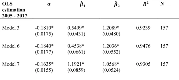
Table 4 Ordinary least square estimations of model 2,3 and 4

OLS estimation 2005 - 2017 a bc b_ ^_ N Model 3 -0.1810* (0.0175) 0.5499* (0.0431) 1.2089* (0.0480) 0.9239 157 Model 6 -0.1840* (0.0177) 0.4538* (0.0661) 1.2036* (0.0552) 0.9476 157 Model 7 -0.1635* (0.0155) 1.1921* (0.0859) 1.0568* (0.0524) 0.9305 157

Note: The estimates above are obtained from the least square regression of equation 3, 6 and 7, The values in parentheses denotes the standard errors. *, indicates the 1 percent significance level of for when we can reject the null hypothesis, - = 0. The sample period is 2005M01 to 20018M01. '4_{is the coefficient of determination, which explains to which}

degree the independent variables explain variance in the dependent, 1= full explanation. N display the number of observation for each regression.

(32)

Table 5. Unit root tests for variables in model 3

MODEL 2

Augmented Dickey-Fuller unit root test

d-statistic ADF test statistic Prob. SX86_RF 1% level 5% level 10% level -3.4725 -2.8799 -2.5766 -0.6519 0.8542 RESINDEX 1% level 5% level 10% level -3.4755 -2.8812 -2.5773 -0.6509 0.8545 OMXSPI_RF 1% level 5% level 10% level -3.4725 -2.8799 -2.5766 -1.3395 0.6103

Note: The table displays the Augmented Dickey-Fuller unit root test for our variables in model 3. The first column displays the test level, the second show the t-statistics, the third displays the ADF statistics that is the critical value used for testing. The ADF test statistic is the critical value used for testing the hypothesis. The last column displays the one-sided probability.

(33)

Table 6. Unit root rests for variables in model 6

MODEL 3

Augmented Dickey-Fuller Unit Root Test

d-statistic ADF test statistic Prob. SX8600PI 1% level 5% level 10% level -3.4725 -2.8799 -2.5766 -0.5144 0.8840 RESINDEX 1% level 5% level 10% level -3.4755 -2.8812 -2.5773 -0.6509 0.8545 OMXSPI 1% level 5% level 10% level -3.4725 -2,8799 -2.5766 -1.1360 0.7008

(34)

Table 7. Unit root rests for variables in model 7

MODEL 4

Augmented

Dickey-Fuller Unit Root Test d-statistic ADF statistic test Prob.

SX86_RF 1% level 5% level 10% level -3.4725 -2.8799 -2.5766 -0.6519 0.8542 RES_IND_RF 1% level 5% level 10% level -3.4755 -2.8812 -2.5773 -0.8744 0.7939 OMXSPI_RF 1% level 5% level 10% level -3.4725 -2.8799 -2.5766 -1.3395 0.6103

(35)

Table 8. Johansen test for cointegration in all our models.

Note: This table displays our results from the Johansen cointegration test. Trace tests indicates one cointegrating equation at the 0.05 significance level for model 3, 6 and 7. Max-Eigenvalue tests indicates one cointegrating equation for all of our models, at the 0.05 significance level. Model 7 Trace statistic None 33.20761 29.79707 0.0195 At most 1 6.84529 15.49471 0.5957 Max-Eigenvalue None 26.36232 21.13162 0.0084 At most 1 6.84123 14.26460 0.5081 Cointergration

Test Test-type Hypothesized number of CE(s) Statistics 0,05 critical value Prob. Model 3 Trace statistic None 31.6958 29.7970 0.0299 At most 1 7.5893 15.4947 0.5103 Max-Eigenvalue None 24.4065 21.1316 0.0185 At most 1 7.3133 14.2646 0.4528 Model 6 Trace statistic None 31.0523 29.79707 0.0357 At most 1 7.3587 15.49471 0.5363