SIMULATION OF RESIDUAL STRESSES
IN CASTINGS
Rubén Lora Echavarría
Jayesh Vasant Namjoshi
THESIS WORK 2007
SIMULATION OF RESIDUAL STRESSES
IN CASTINGS
Rubén Lora Echavarría
Jayesh Vasant Namjoshi
This thesis work is performed at the Jönköping Institute of Technology within the subject area of Machine Technology. The work is part of the university’s Master of Science with a Mayor in Mechanical Engineering Specializing in Product Development and Industrial Design.
The authors are responsible for the given opinions, conclusions and results. Supervisor: Niclas Strömberg
Credit points: 30 points Date: 21-January-2008 Archive number:
Abstract
This work presents a study and implementation of the simulation of residual stresses in castings. The objects of study are a cast iron truck Hub part (provided by the company Volvo 3P) and an optimized version of the Hub resulting from the application of a topology optimization process. The models are solved through an uncoupled thermo-mechanical solidification analysis, performed both in the FE commercial software Abaqus and the FD commercial software Magmasoft and the results are compared. First, a thermal analysis is carried out where the casting is cooled down from a super-heated temperature to room temperature. The thermal history obtained, is then used as an external force to calculate the residual stresses by means of a quasi-static mechanical analysis, using a J2-plasticity model. The simulation procedures are explained through a simplified model of the Hub and then applied to the geometries of interest. A results comparison between the original Hub and its optimized version is also presented. The theoretical base is given in this work as well as detailed implementation procedures. The results shows that the part subjected to the topology optimization process develop less residual stresses than its original version.
Key Words
Key Words
Residual stresses • Thermo-mechanical • Quasi-static • Castings • FEM • FDM • Numerical simulation • Solidification • Thermal analysis • Stress analysis • Meshing • Abaqus • Magmasoft • Hypermesh • Matlab • ProEngineer
Table of Contents
1 Introduction... 1
1.1BACKGROUND...2
1.2PURPOSE AND AIMS...3
1.3DELIMITS...3 2 Theoretical background ... 4 2.1THE THERMAL ANALYSIS...4 2.1.1 Heat transference...4 2.1.1.1 Conduction ... 4 2.1.1.2 Convection ... 5 2.1.1.3 Radiation ... 5 2.1.2 Material properties ...7 2.1.2.1 Thermal conductivity (k)... 7 2.1.2.2 Density (ρ)... 7
2.1.2.3 Specific Heat (cv and cp)... 7
2.1.2.4 Latent Heat (L)... 8
2.1.2.5 Thermal diffusivity (α)... 8
2.1.3 Initial and Boundary conditions ...9
2.1.3.1 Prescribed boundary temperature ... 9
2.1.3.2 Perfectly insulated (adiabatic) boundary ... 9
2.1.3.3 Convection boundary condition ... 10
2.1.3.4 Radiation boundary condition ... 10
2.1.3.5 Internal boundary (two solids bodies in contact) condition... 10
2.1.4 The Heat Conduction Equation...11
2.1.4.1 1-D transient (time dependent) heat conduction equation ... 11
2.1.4.2 1-D steady-state heat conduction equation ... 11
2.1.4.3 The 3-D transient Heat Conduction Equation... 11
2.1.5 Numerical solutions ...12
2.1.5.1 Finite element method... 12
2.1.5.2 Finite difference method ... 13
2.2THE STRESS ANALYSIS...14 2.2.1 Residual Stresses...14 2.2.2 Elasticity ...14 2.2.2.1 Elastic strain... 14 2.2.2.2 Thermal strain ... 15 2.2.3 Plasticity...15 2.2.3.1 Ideal Plasticity... 15 2.2.3.2 Hardening... 17
2.2.3.3 Temperature Dependent Yield Stress ... 17
2.2.3.4 Plasticity Material models ... 18
2.2.3.4.1 The Yield Surface ... 18
2.2.3.4.2 Illustration for a Simple Mathematical Model ... 18
2.2.3.5 J2-Plasticty model ... 21
2.2.3.5.1 J2-Plasticity model - Constitutive Laws... 21
3 Implementation... 23 3.1PROCESS SUMMARY...23 3.2PROCEDURE...25 4 Cylinder Results ... 26 4.1GEOMETRY...26 4.2MESH...27 4.3BOUNDARY CONDITIONS...28
4.3.1 Thermal boundary conditions ...28
Table of Contents
4.3.2 Mechanical boundary conditions ...29
4.3.2.1 Stress analysis step ... 29
4.4COOLING CURVES...32
4.5THERMAL COLOR SPECTRUMS...33
4.6STRESS CURVES...34
4.7STRESS COLOR SPECTRUMS...36
4.8SIMULATION TIME FOR THE CYLINDER...39
5 Original Hub Results... 40
5.1GEOMETRY...40
5.2THERMAL AND STRESS CURVES POINTS PLACEMENT...42
5.3MESH...42
5.4BOUNDARY CONDITIONS...45
5.4.1 Thermal boundary conditions ...45
5.4.1.1 Before Shake-out... 45
5.4.1.2 After shake out ... 45
5.4.2 Mechanical boundary conditions ...46
5.4.2.1 Stress analysis step ... 46
5.5COOLING CURVES FOR THE ORIGINAL HUB...49
5.6THERMAL COLOR SPECTRUMS...50
5.7STRESS CURVES FOR THE ORIGINAL HUB...52
5.8STRESS COLOR SPECTRUMS...54
5.9SIMULATION TIME OF THE ORIGINAL HUB...60
6 Optimized Hub Results ... 61
6.1GEOMETRY...61
6.2THERMAL AND STRESS CURVES POINTS PLACEMENT...62
6.3MESH...63
6.4BOUNDARY CONDITIONS...66
6.4.1 Thermal boundary conditions ...66
6.4.1.1 Before Shake-out... 66
6.4.1.2 After shake out ... 66
6.4.2 Mechanical boundary conditions ...67
6.4.2.1 Stress analysis step ... 67
6.5COOLING CURVES FOR THE OPTIMIZED HUB...70
6.6THERMAL COLOR SPECTRUMS...71
6.7STRESS CURVES FOR THE OPTIMIZED HUB...73
6.8STRESS COLOR SPECTRUMS...75
6.9SIMULATION TIME OF THE OPTIMIZED HUB...81
7 Original and Optimized Hub Comparison... 82
7.1MISES...82
7.2MAXIMUM PRINCIPAL STRESS...85
7.3MINIMUM PRINCIPAL STRESS...88
8 Conclusions and discussions... 91
9 References... 92 10 Appendix ... 94 10.1ABAQUS IMPLEMENTATION...94 10.1.1 Pre-Processing...95 10.1.1.1 Geometry Definition ... 95 10.1.1.2 Mesh Generation ... 97
10.1.1.2.1 Importing the Geometry... 98
10.1.1.2.2 Geometry Cleanup ... 99
10.1.1.2.3 Organizing the model... 99
10.1.1.2.4 Meshing the surfaces... 101
10.1.1.2.6 Exporting the meshes to Abaqus ... 108
10.1.1.3 Abaqus Simulation Setup ... 110
10.1.1.3.1 The Thermal Simulation ... 110
10.1.1.3.1.1 Before Shake-Out model... 111
10.1.1.3.1.2 After Shake-Out model ... 126
10.1.1.3.2 The Stress Simulation ... 131
10.1.2 Calculation ...140
10.1.3 Post-Processing ...141
10.1.3.1 Results Visualization... 141
10.1.3.1.1 Loading the Output Data Base ... 141
10.1.3.1.2 Cut Sections ... 143
10.1.3.1.3 Removing a part from the viewport ... 143
10.1.3.1.4 Creating X-Y Curves ... 144
10.1.3.2 Results Preparation for Comparison... 145
10.1.3.2.1 Saving a curve... 146
10.1.3.2.2 Exporting the curves ... 146
10.2MAGMASOFT IMPLEMENTATION...148
10.2.1 Pre-Processing...148
10.2.1.1 Geometry Definition ... 148
10.2.1.2 Mesh Generation ... 153
10.2.1.3 Magmasoft Simulation Setup ... 154
10.2.2 Calculation ...162
10.2.3 Post-Processing ...163
10.2.3.1 Results Visualization... 163
10.2.3.1.1 Creating a cut view: ... 165
10.2.3.1.2 The curves:... 167
10.2.3.2 Results Preparation for Comparison... 169
10.2.3.2.1 Exporting a curve:... 169
10.3RESULTS COMPARISON APPROACH...170
10.3.1 Thermal Results Comparison Approach ...171
10.3.1.1 Combining the Abaqus thermal results... 171
10.3.1.1.1 Loading the Abaqus .rpt files into Excel ... 171
10.3.1.1.2 Combining the Before and After Shake-Out Abaqus .rpt files... 173
10.3.1.2 Loading the Magma .txt file into Excel ... 173
10.3.1.3 Setting up the Matlab M-File ... 175
10.3.1.4 Plotting the comparison... 177
10.3.1.5 Exporting the comparison image... 177
10.3.2 Stress results comparison approach...177
10.3.2.1.1 Loading the Abaqus .rpt files into Excel ... 177
10.3.2.2 Loading the Magma .txt file into Excel ... 177
10.3.2.3 Modifying the units of the Magma XY data... 178
10.3.2.4 Setting the Matlab M-File ... 179
10.3.2.5 Plotting the comparison... 179
10.3.2.6 Exporting the comparison image... 179
10.4MATERIAL DATA...180
10.4.1 Thermal Material Data ...180
10.4.2 Stress Material Data ...182
10.5KEYWORDS OF THE ABAQUS INPUT FILES...186
10.6THERMAL EXPANSION COEFFICIENT CALCULATION MAGMASOFT -ABAQUS...196
10.7CONDUCTION INTERACTION VS TIE CONSTRAINT...198
10.8RESULTS COMPARISON WITH AND WITHOUT SYMMETRY...199
10.8.1 Cylinder...199 10.8.1.1 Geometry... 199 10.8.1.2 Simulation time ... 200 10.8.1.3 Thermal results... 200 10.8.1.4 Stress results... 201 10.8.2 Original Hub ...203 10.8.2.1 Geometry... 203 10.8.2.2 Simulation time ... 203 10.8.2.3 Stress results... 204 10.8.3 Optimized Hub...206 10.8.3.1 Geometry... 206 10.8.3.2 Simulation time ... 206 10.8.3.3 Thermal results... 207
Table of Contents
Figures Table
FIGURE 2.1.IDEAL PLASTICITY...16
FIGURE 2.2.LINEAR HARDENING...17
FIGURE 2.3.STRESS-TRAIN CURVES AT DIFFERENT TEMPERATURES, LINEAR HARDENING APPROACH...17
FIGURE 2.4.ONE DIMENSIONAL FRICTIONAL DEVICE REPRESENTING IDEAL PLASTICITY...19
FIGURE 3.1.STEPS SEQUENCE FOR RESIDUAL STRESS ANALYSIS...25
FIGURE 4.1.THE CYLINDER PART.UNITS:METERS...26
FIGURE 4.2.THE MOLD PART.UNITS:METERS...26
FIGURE 4.3.HYPERMESH MESH USED IN ABAQUS...27
FIGURE 4.4.MAGMASOFT MESH...27
FIGURE 4.5.CONSTRAINING THE RIGID BODY TRANSLATIONS IN X,Y AND Z IN THE CYLINDER...29
FIGURE 4.6.CONSTRAINING THE ROTATIONS IN Y AND Z IN A SINGLE NODE SELECTION (IN RED) FOR THE CYLINDER MODEL...30
FIGURE 4.7.CONSTRAINING THE ROTATIONS IN X IN A SINGLE NODE SELECTION (IN RED) FOR THE CYLINDER MODEL...31
FIGURE 4.8.ABAQUS VS.MAGMASOFT COOLING CURVES FOR THE CYLINDER MODEL...32
FIGURE 4.9.ABAQUS (TOP) AND MAGMASOFT (BOTTOM) THERMAL COLOR SPECTRUMS OF THE LAST STEP AFTER SHAKE OUT OF THE CYLINDER MODEL. ...33
FIGURE 4.10.ABAQUS VS.MAGMA VON MISES CURVES FOR THE CYLINDER MODEL...34
FIGURE 4.11.ABAQUS VS.MAGMA MAXIMUM PRINCIPAL STRESSES FOR THE CYLINDER MODEL...34
FIGURE 4.12.ABAQUS VS.MAGMA MINIMUM PRINCIPAL STRESSES FOR THE CYLINDER MODEL...35
FIGURE 4.13.ABAQUS (TOP) AND MAGMASOFT (BOTTOM) COLOR SPECTRUMS FOR THE MISES RESULTS OF THE CYLINDER MODEL...36
FIGURE 4.14.ABAQUS (TOP) AND MAGMASOFT (BOTTOM) COLOR SPECTRUMS FOR THE RESIDUAL MAXIMUM PRINCIPAL STRESSES OF THE CYLINDER MODEL...37
FIGURE 4.15.ABAQUS (TOP) AND MAGMASOFT (BOTTOM) COLOR SPECTRUMS FOR THE RESIDUAL MIN. PRINCIPAL STRESSES OF THE CYLINDER MODEL. ...38
FIGURE 5.1.FRONT AND TOP VIEW OF THE ORIGINAL HUB MODEL...40
FIGURE 5.2.BOTTOM VIEW OF THE ORIGINAL HUB MODEL...41
FIGURE 5.3.THE HUB MOLD PART.UNITS:METERS...41
FIGURE 5.4.LOCATION OF THE COOLING AND STRESS POINTS OF THE HUB PART...42
FIGURE 5.5.MESH OF THE HUB MODEL USED IN ABAQUS...43
FIGURE 5.6.MAGMASOFT MESH OF THE HUB MODEL...44
FIGURE 5.7.CONSTRAINING THE RIGID BODY TRANSLATIONS IN X,Y AND Z IN THE OPTIMIZED HUB....46
FIGURE 5.8.CONSTRAINING THE ROTATIONS IN THE X AND Z AXES IN THE ORIGINAL HUB...47
FIGURE 5.9.CONSTRAINING THE ROTATION IN THE X AXIS IN THE ORIGINAL HUB...48
FIGURE 5.10.ABAQUS VS.MAGMASOFT COOLING CURVES FOR THE HUB MODEL...49
FIGURE 5.11.ABAQUS THERMAL COLOR SPECTRUMS FOR THE LAST STEP AFTER SHAKE-OUT OF THE ORIGINAL HUB MODEL...50
FIGURE 5.12.MAGMASOFT THERMAL COLOR SPECTRUMS FOR THE LAST STEP AFTER SHAKE-OUT OF THE ORIGINAL HUB MODEL...51
FIGURE 5.13.VON MISES CURVES FROM PNT0 OF THE ORIGINAL HUB. ...52
FIGURE 5.14.MAXIMUM PRINCIPAL STRESSES FROM PNT0 OF THE ORIGINAL HUB. ...52
FIGURE 5.15.MINIMUM PRINCIPAL STRESSES FROM PNT0 OF THE ORIGINAL HUB. ...53
FIGURE 5.16.ABAQUS COLOR SPECTRUMS FOR THE MISES RESULTS OF THE ORIGINAL HUB. ...54
FIGURE 5.17.MAGMASOFT COLOR SPECTRUMS FOR THE MISES RESULTS OF THE ORIGINAL HUB...55
FIGURE 5.18.ABAQUS COLOR SPECTRUMS FOR THE RESIDUAL MAX.PRINCIPAL STRESSES OF THE ORIGINAL HUB. ...56
FIGURE 5.19.MAGMASOFT COLOR SPECTRUMS FOR THE RESIDUAL MAX.PRINCIPAL STRESSES OF THE ORIGINAL HUB. ...57
FIGURE 5.20.ABAQUS COLOR SPECTRUMS FOR THE RESIDUAL MIN.PRINCIPAL STRESSES OF THE ORIGINAL HUB. ...58
FIGURE 5.21.MAGMASOFT COLOR SPECTRUMS FOR THE RESIDUAL MIN.PRINCIPAL STRESSES OF THE ORIGINAL HUB. ...59
FIGURE 6.2.BOTTOM VIEW OF THE OPTIMIZED HUB MODEL...62
FIGURE 6.3.LOCATION OF COOLING AND STRESS POINTS 5 AND 6 FOR THE OPTIMIZED HUB. ...62
FIGURE 6.4.MESH OF THE OPTIMIZED HUB MODEL USED IN ABAQUS...64
FIGURE 6.5.MAGMA MESH OF THE OPTIMIZED HUB MODEL. ...65
FIGURE 6.6.CONSTRAINING THE RIGID BODY TRANSLATIONS IN X,Y AND Z IN THE OPTIMIZED HUB....67
FIGURE 6.7.CONSTRAINING THE ROTATIONS IN THE Y AND Z AXES IN THE OPTIMIZED HUB...68
FIGURE 6.8.CONSTRAINING THE ROTATION IN THE X AXIS IN THE OPTIMIZED HUB...69
FIGURE 6.9.ABAQUS VS.MAGMASOFT COOLING CURVES FOR THE OPTIMIZED HUB MODEL...70
FIGURE 6.10.ABAQUS THERMAL COLOR SPECTRUMS FOR THE LAST STEP AFTER SHAKE-OUT OF THE OPTIMIZED HUB MODEL...71
FIGURE 6.11.MAGMASOFT THERMAL COLOR SPECTRUMS FOR THE LAST STEP AFTER SHAKE-OUT OF THE OPTIMIZED HUB MODEL...72
FIGURE 6.12.VON MISES CURVES FROM PNT5 OF THE OPTIMIZED HUB...73
FIGURE 6.13.MAXIMUM PRINCIPAL STRESSES FROM PNT5 OF THE OPTIMIZED HUB...73
FIGURE 6.14.MINIMUM PRINCIPAL STRESSES FROM PNT5 OF THE OPTIMIZED HUB...74
FIGURE 6.15.ABAQUS COLOR SPECTRUMS FOR THE MISES RESULTS OF THE OPTIMIZED HUB. ...75
FIGURE 6.16.MAGMASOFT COLOR SPECTRUMS FOR THE MISES RESULTS OF THE OPTIMIZED HUB...76
FIGURE 6.17.ABAQUS COLOR SPECTRUMS FOR THE RESIDUAL MAX.PRINCIPAL STRESSES OF THE OPTIMIZED HUB...77
FIGURE 6.18.MAGMASOFT COLOR SPECTRUMS FOR THE RESIDUAL MAX.PRINCIPAL STRESSES OF THE OPTIMIZED HUB...78
FIGURE 6.19.ABAQUS COLOR SPECTRUMS FOR THE RESIDUAL MIN.PRINCIPAL STRESSES OF THE OPTIMIZED HUB...79
FIGURE 6.20.MAGMASOFT COLOR SPECTRUMS FOR THE RESIDUAL MIN.PRINCIPAL STRESSES OF THE OPTIMIZED HUB...80
FIGURE 7.1.ORIGINAL HUB (TOP) AND OPTIMIZED HUB (BOTTOM)MISES COMPARISON.TOP VIEW. ...82
FIGURE 7.2.ORIGINAL HUB (TOP) AND OPTIMIZED HUB (BOTTOM)MISES COMPARISON.BOTTOM VIEW. ...83
FIGURE 7.3.ORIGINAL HUB (TOP) AND OPTIMIZED HUB (BOTTOM)MISES COMPARISON.INCLINED VIEW. ...84
FIGURE 7.4.ORIGINAL HUB (TOP) AND OPTIMIZED HUB (BOTTOM)MAXIMUM PRINCIPAL STRESS COMPARISON.TOP VIEW. ...85
FIGURE 7.5.ORIGINAL HUB (TOP) AND OPTIMIZED HUB (BOTTOM)MAXIMUM PRINCIPAL STRESS COMPARISON.BOTTOM VIEW...86
FIGURE 7.6.ORIGINAL HUB (TOP) AND OPTIMIZED HUB (BOTTOM)MAXIMUM PRINCIPAL STRESS COMPARISON.INCLINED VIEW...87
FIGURE 7.7.ORIGINAL HUB (TOP) AND OPTIMIZED HUB (BOTTOM)MINIMUM PRINCIPAL STRESS COMPARISON.TOP VIEW. ...88
FIGURE 7.8.ORIGINAL HUB (TOP) AND OPTIMIZED HUB (BOTTOM)MINIMUM PRINCIPAL STRESS COMPARISON.BOTTOM VIEW...89
FIGURE 7.9.ORIGINAL HUB (TOP) AND OPTIMIZED HUB (BOTTOM)MINIMUM PRINCIPAL STRESS COMPARISON.INCLINED VIEW...90
FIGURE 10.1.STEPS SEQUENCE FOR THE RESIDUAL STRESS ANALYSIS...94
FIGURE 10.2.THE CYLINDER PART.UNITS:METERS...95
FIGURE 10.3.THE CYLINDER MOLD PART.UNITS:METERS...95
FIGURE 10.4.STL EXPORT WINDOW,PROENGINEER...97
FIGURE 10.5.USER PROFILES WINDOW...98
FIGURE 10.6.WIREFRAME APPEARANCE OF THE .STL GEOMETRY OF THE MOLD IN HYPERMESH...98
FIGURE 10.7.GENERAL APPEARANCE OF THE AUTO CLEANUP PANEL...99
FIGURE 10.8.COLLECTORS OF THE MOLD_SURF_MESH.HM MODEL IN HYPERMESH...100
FIGURE 10.9.AUTOMESH PANEL (IS DIVIDED IN TWO FOR DISPLAY PURPOSES). ...101
FIGURE 10.10.MOLD_SURF_MESH.HM MODEL...102
FIGURE 10.11.CYLINDER_SURF_MESH.HM MODEL...103
FIGURE 10.12.TETRAMESH PANEL SETTING FOR THE “CYLINDER_VOLUME_MESH.HM” MODEL...104
FIGURE 10.13.A MASKED VIEW OF THE CYLINDER MODEL WHERE INNER ELEMENTS CAN BE SEEN...105
FIGURE 10.14.TETRAMESH PANEL SETTING FOR THE “MOLD_VOLUME_MESH.HM” MODEL...106
FIGURE 10.15.A MASKED VIEW OF THE MOLD MODEL WHERE INNER ELEMENTS CAN BE SEEN...107
FIGURE 10.16.UTILITY BROWSER APPEARANCE FOR THE ABAQUS USER PROFILE...108
FIGURE 10.17.IMPORTED CAD FILES IN ABAQUS...112
Table of Contents
FIGURE 10.19.CONDUCTIVITY MATERIAL DATA CURVE FOR THE CYLINDER PART...114
FIGURE 10.20.SPECIFIC HEAT MATERIAL DATA CURVE FOR THE CYLINDER PART...115
FIGURE 10.21.DENSITY MATERIAL DATA CURVE FOR THE MOLD PART...115
FIGURE 10.22.CONDUCTIVITY MATERIAL DATA CURVE FOR THE MOLD PART...116
FIGURE 10.23.SPECIFIC HEAT MATERIAL DATA CURVE FOR THE MOLD PART...116
FIGURE 10.24.SELECTION OPTION TOOLS. ...117
FIGURE 10.25.MODEL TREE AFTER COMPLETING THE FIRST 5 STEPS OF THE SETUP...119
FIGURE 10.26.HTC–CONDUCTION INTERACTION PROPERTY BETWEEN THE CAST AND THE MOLD...121
FIGURE 10.27.CONDUCTIVE INTERACTION BETWEEN THE CAST AND THE MOLD...123
FIGURE 10.28.CONVECTIVE INTERACTION BETWEEN THE MOLD AND THE AMBIENT...123
FIGURE 10.29.RADIATION INTERACTION BETWEEN THE MOLD AND THE AMBIENT...124
FIGURE 10.30.FIELD OUTPUT REQUEST OF THE NODAL THERMAL HISTORY. ...125
FIGURE 10.31.CONVECTIVE INTERACTION PROPERTY BETWEEN THE CASTING AND THE AMBIENT. ...129
FIGURE 10.32.CAST-AMBIENT-CONVECTION INTERACTION...130
FIGURE 10.33.CAST-AMBIENT-RADIATION INTERACTION...130
FIGURE 10.34.YOUNG MODULUS MATERIAL DATA CURVE FOR THE CYLINDER PART...132
FIGURE 10.35.POISSON’S RATIO MATERIAL DATA CURVE FOR THE CYLINDER PART...133
FIGURE 10.36.THERMAL EXPANSION COEFFICIENT MATERIAL DATA CURVE FOR THE CYLINDER PART133 FIGURE 10.37.PLASTICITY MATERIAL DATA CURVE FOR THE CYLINDER PART...134
FIGURE 10.38.TOTALLY CONSTRAINED NODE.BOUNDARY CONDITIONS,STRESS ANALYSIS...137
FIGURE 10.39.EDIT BOUNDARY CONDITIONS WINDOW FOR A FULLY CONSTRAINED NODE. ...137
FIGURE 10.40.SEMI-FIXED NODE (RED) ALIGNED IN THE X DIRECTION WITH THE TOTALLY FIXED ONE 138 FIGURE 10.41.SEMI-FIXED NODE ALIGNED IN Z WITH THE TOTALLY CONSTRAINED ONE...138
FIGURE 10.42.FIELD OUTPUT REQUEST CONFIGURATION FOR THE III-STRESS MODEL...139
FIGURE 10.43.JOB STATUS...140
FIGURE 10.44.AN .ODB IN THE RESULTS TREE...142
FIGURE 10.45.“PLOT CONTOURS ON DEFORMED SHAPE” BUTTON (SELECTED)...142
FIGURE 10.46. “VIEW CUT MANAGER” BUTTON (SELECTED) ...143
FIGURE 10.47.VIEW CUT MANAGER WINDOW...143
FIGURE 10.48.VARIABLES TAB IN THE XYDATA FROM ODBOUTPUT WINDOW...145
FIGURE 10.49.ELEMENTS/NODES TAB IN THE XYDATA FROM ODBOUTPUT WINDOW...146
FIGURE 10.50.REPORT XYDATA WINDOW...147
FIGURE 10.51.STEPS SEQUENCE FOR THE RESIDUAL STRESS ANALYSIS...148
FIGURE 10.52.TYPICAL APPEARANCE OF THE MAGMASOFT MAIN INTERFACE...149
FIGURE 10.53.MAGMA_CYLINDER.STL FILE IMPORTED INTO THE MAGMASOFT PREPROCESSOR...150
FIGURE 10.54.LOCATION OF THE MATERIAL BUTTON IN THE PREPROCESSOR INTERFACE...150
FIGURE 10.55.ENTITY SELECTIONS WINDOWS WITH THE VOLUMES SELECTED PRIOR ORGANIZING...152
FIGURE 10.56.MAGMASOFT MESH GENERATION WINDOW...153
FIGURE 10.57.PROCESS MODE WINDOW...154
FIGURE 10.58.THE “MATERIAL DEFINITIONS” WINDOW...155
FIGURE 10.59.DATABASE REQUEST WINDOW...155
FIGURE 10.60.MAGMADATA WINDOW FOR THE PROJECT DATABASE...156
FIGURE 10.61.DEFAULT YOUNG’S MODULUS FOR THE GJL-150 MATERIAL...157
FIGURE 10.62.GJL-150 MATERIAL SELECTED FROM THE PROJECT DATABASE IN THE DATABASE REQUEST WINDOW...157
FIGURE 10.63.HEAT TRANSFER DEFINITIONS WINDOW...158
FIGURE 10.64.OPTIONS WINDOW...159
FIGURE 10.65.SHAKE OUT DEFINITIONS WINDOW...159
FIGURE 10.66.SHAKE OUT OPTIONS WINDOW...160
FIGURE 10.67.STORING DATA DEFINITIONS WINDOW...160
FIGURE 10.68.SOLIDIFICATION DEFINITIONS WINDOW...161
FIGURE 10.69.STRESS SIMULATION OPTIONS WINDOW...161
FIGURE 10.70.FAST POSTPROCESSING PREPARATION WINDOW...162
FIGURE 10.71.ACIS® CONVERTER WINDOW...163
FIGURE 10.72.POSTPROCESSOR MAIN INTERFACE...164
FIGURE 10.73.RESULTS TAB SELECTED IN THE POSTPROCESSOR’S CONTROL PANEL WINDOW...164
FIGURE 10.74.TEMPERATURE FIELD RESULT DISPLAYED IN THE POSTPROCESSOR’S MAIN WINDOW...165
FIGURE 10.75.CUT VIEW SETTING WITH THE SLICE FUNCTIONALITY...166
FIGURE 10.76.CUT VIEW DISPLAYED IN THE MAIN WINDOW...166
FIGURE 10.78.COOLING CURVE DISPLAY IN THE POSTPROCESSOR MAIN WINDOW...168
FIGURE 10.79.EXPORTING THE CURVES FROM THE CURVE’S OPTIONS TAB...169
FIGURE 10.80.IMPORTING AN .RPT FILE INTO EXCEL.TEXT IMPORT WIZARD STEP 1 OF 3 WINDOW...171
FIGURE 10.81.IMPORTING AN .RPT FILE INTO EXCEL.TEXT IMPORT WIZARD STEP 2 OF 3 WINDOW...172
FIGURE 10.82.IMPORTING AN .RPT FILE INTO EXCEL.TEXT IMPORT WIZARD STEP 3 OF 3 WINDOW...172
FIGURE 10.83.IMPORTING AN .TXT FILE INTO EXCEL.TEXT IMPORT WIZARD STEP 1 OF 3 WINDOW...173
FIGURE 10.84.IMPORTING AN .TXT FILE INTO EXCEL.TEXT IMPORT WIZARD STEP 2 OF 3 WINDOW...174
FIGURE 10.85.IMPORTING AN .TXT FILE INTO EXCEL.TEXT IMPORT WIZARD STEP 3 OF 3 WINDOW...174
FIGURE 10.86.TEMPLATE CODE FOR THE THERMAL COMPARISON...175
FIGURE 10.87.EXAMPLE OF A POPULATED VECTOR...176
FIGURE 10.88.CHANGING MAGMASOFT STRESS CURVE RESULTS FROM MPA TO PA. ...178
FIGURE 10.89.COMPARISON BETWEEN CONDUCTION INTERACTION WITH HTC=1000,TIE CONSTRAINT AND MAGMASOFT HTC=1000...198
FIGURE 10.90.1/8TH OF THE CYLINDER GEOMETRY AS USED IN THE SYMMETRY ANALYSIS...199
FIGURE 10.91.THERMAL RESULTS COMPARISON OF THE CYLINDER MODEL WITH AND WITHOUT SYMMETRY...200
FIGURE 10.92.MISES COMPARISON OF THE CYLINDER MODEL WITH AND WITHOUT SYMMETRY...201
FIGURE 10.93.MAXIMUM PRINCIPAL STRESS COMPARISON OF THE CYLINDER MODEL WITH AND WITHOUT SYMMETRY...201
FIGURE 10.94.MINIMUM PRINCIPAL STRESS COMPARISON OF THE CYLINDER MODEL WITH AND WITHOUT SYMMETRY...202
FIGURE 10.95.HALF OF THE ORIGINAL HUB GEOMETRY AS USED IN THE SYMMETRY ANALYSIS...203
FIGURE 10.96.MISES COMPARISON OF THE ORIGINAL HUB MODEL WITH AND WITHOUT SYMMETRY...204
FIGURE 10.97.MAXIMUM PRINCIPAL STRESS COMPARISON OF THE ORIGINAL HUB MODEL WITH AND WITHOUT SYMMETRY...204
FIGURE 10.98.MINIMUM PRINCIPAL STRESS COMPARISON OF THE ORIGINAL HUB MODEL WITH AND WITHOUT SYMMETRY...205
FIGURE 10.99.HALF OF THE OPTIMIZED HUB GEOMETRY AS USED IN THE SYMMETRY ANALYSIS...206
FIGURE 10.100.THERMAL RESULTS COMPARISON OF THE OPTIMIZED HUB MODEL WITH AND WITHOUT SYMMETRY...207
FIGURE 10.101.MISES COMPARISON OF THE OPTIMIZED HUB MODEL WITH AND WITHOUT SYMMETRY208 FIGURE 10.102.MAXIMUM PRINCIPAL STRESS COMPARISON OF THE OPTIMIZED HUB MODEL WITH AND WITHOUT SYMMETRY...208
FIGURE 10.103.MINIMUM PRINCIPAL STRESS COMPARISON OF THE OPTIMIZED HUB MODEL WITH AND WITHOUT SYMMETRY...209
Introduction
1
Introduction
During the solidification process of castings, residual stresses are developed due to temperature gradients between different parts of the casting, mechanical
constraints imposed by the mold during shrinkage of the cast metal, and volumetric change and transformation plasticity associated with the solid state phase transformation according to Chandra U., Ahmed A. (2002). Since the residual stresses can increase or decrease the fatigue life of a component, an interest on its consideration during the design process has grown in the industry of casted parts. Scientific information supporting the validity of such interest is offered in Gustafsson E., Hofwing M., Stromberg N. (2007).
Considerable differences, when residual stresses are included or not in shape optimization processes of castings, has been presented in Chandra U., Ahmed A. (2002),
Modelling for casting and solidification processing,
Marcel Dekker, New York
Gustafsson E., Stromberg N. (2006). Differences between results of residual stresses obtained from the commercial softwares Abaqus and Magmasoft are also presented in Gustafsson E., Hofwing M., Stromberg N. (2007).
This work presents a comparison of residual stress development between parts that has and has not undergone topology optimization processes. As well, we provide a detailed procedure to carry out residual stress simulations, both in Abaqus and Magmasoft including the steps for the geometry preparation, mesh generation and results comparison using ProEngineer, Hypermesh and Matlab respectively. The results obtained from the two solvers are also compared and the theoretical fundamentals are given.
The residual stresses are calculated using an uncoupled thermo-mechanical solidification analysis. A thermal analysis is performed first and then, the thermal history is read into a quasi-static mechanical analysis to calculate the residual stresses, using a J2-plasticity model.
An academic problem is set using a simple geometry to implement and explain the procedure. Then, residual stresses are calculated on the truck Hub part provided by Volvo 3P, and finally the same simulation is performed on a topologically optimized version of the mentioned part.
1.1 Background
The thermal analysis
The governing equation for the thermal analysis is the classical heat equation ] [k T div t T T H = ∇ ∂ ∂ ∂ ∂ ρ (1.1)
Where ρ , H and k are temperature dependent and represent density, enthalpy and thermal conductivity respectively. T is the temperature and t is the time.
The stress analysis
The equilibrium equation for the residual stress analysis is
0 ] [σ =
div (1.2)
Where σ is the stress tensor.
The yield surface equation for the J2-plasticity model reads
(
,)
= 3 2 − − − ≤0 y p h J T f σ ε σ (1.3)Where J2 is the second invariant of the deviatoric stress tensor, h is the temperature dependent hardening parameter, ε−p is the equivalent plastic strain and σ is the y
Introduction
1.2 Purpose and aims
1-Compare the residual stress development of parts subjected and not subjected to topology optimization processes.
2-Present a methodology to perform numerical simulations of residual stresses. 3-Compare solutions obtained from the FE solver Abaqus and the FD solver Magmasoft.
1.3 Delimits
For the purpose of our work, a general understanding of the Finite Element and the Finite Difference formulations are sufficient. This work does not present the mathematical details of the FE or the FD method.
No details about the topology optimization process are intended to be provided in this work. The topologically optimized version of the part provided by Volvo 3P was given.
2
Theoretical background
2.1 The Thermal Analysis
This chapter aims to provide basic information related with the simulation of solidification in castings about heat transfer mechanisms, material properties, boundary conditions, the heat conduction equation and the numerical methods.
2.1.1 Heat transference
When a system is at a different temperature than its surroundings, the Nature tries to reach thermal equilibrium. To do so, as the second law of thermodynamics explains, the thermal energy always moves from the system of higher temperature to the system of lower temperature.
This transfer of thermal energy occurs due to one or a combination of the three basic heat transport mechanisms: Conduction, Convection and Radiation.
2.1.1.1 Conduction
Is the transference of heat through direct molecular communication, i.e. by physical contact of the particles within a medium or between mediums. It takes place in gases, liquids and solids. In conduction, there is no flow of any of the material mediums.
The governing equation for conduction is called the Fourier’s law of heat conduction and it express that the heat flow per unit area is proportional to the normal temperature gradient, where the proportionality constant is the thermal conductivity: x T kA q ∂ ∂ − = (2.1)
Where q is the heat flux perpendicular to a surface of area A, [W]; A is the surface area through which the heat flow occurs, [m2] ; k is the thermal conductivity, [W/(mK)]; T is the temperature, [K] or [°C]; and x is the perpendicular distance
Theoretical Background
2.1.1.2 Convection
Is the heat transfer by mass motion of a fluid when the heated fluid moves away from the heat source. It combines conduction with the effect of a current of fluid that moves its heated particles to cooler areas and replace them by cooler ones. The flow can be either due to buoyancy forces (natural convection) or due to artificially induced currents (forced convection).
The equation that represents convection comes from the Newton’s law of cooling and is of the form:
(
T Ts)
hA
q=− ∞ − (2.2)
Where h is the convective heat transfer coefficient [W/(m2
K)]; is the
temperature of the cooling fluid; and Ts is the temperature of the surface of the body.
∞ T
2.1.1.3 Radiation
In general, radiation is energy in the form of waves or moving subatomic particles. Among the radiation types, we are specifically interested in the Thermal radiation. Thermal radiation is heat transfer by the emission of electromagnetic waves from the surface of an object due to temperature differences which carry energy away from the emitting object.
The basic relationship governing radiation from hot objects is called the Stefan-Boltzmann law:
(
4)
2 4 1 T T A q=εσ − (2.3)Where ε is the coefficient of emissivity (=1 for ideal radiator); σ is the Stefan-Boltzmann constant of proportionality (5.669E-8 [W/(m2K4)]); A is the radiating surface area; T1 is the temperature of the radiator; and T2 is the temperature of the surroundings.
The three of the previously mentioned heat transport mechanisms can be
expressed by the model law that state that a flux is proportional to a difference in driving potential divided by a resistance, in our case:
th
R T
q=−Δ (2.4)
Being the Thermal Resistance (Rth) for each one of them as follow: kA x Rcond th Δ = (2.5) A h R conv conv th 1 = (2.6) A h R rad rad th 1 = (2.7)
Where hrad is:
(
3)
2 2 2 1 2 2 1 3 1 T T TT T T hrad =εσ + + + (2.8)Theoretical Background
2.1.2 Material properties
2.1.2.1 Thermal conductivity (k)
Is the ability of a material to conduct heat. It is defined as the quantity of heat,
Q, transmitted during a period of time
Δ Δt through a thickness L, in a direction
normal to a surface of area A, due to a temperature difference ΔT, under steady
state conditions and when the heat transfer is dependent only on the temperature gradient. T A L t Q k Δ × × Δ Δ = [W/mK] (2.9)
2.1.2.2 Density (ρ)
Indicate the mass per unit volume of a material.
V m
=
ρ [Kg/m3
] (2.10)
Density is a temperature and pressure dependent material property. In solids and liquids is just slightly affected by these factors but in gases is strongly dependent in both of them.
2.1.2.3 Specific Heat (c
vand c
p)
In general, is the measure of the heat energy required to increase the temperature of a unit quantity of a substance by a defined temperature step. For example, how much heat must be added to increase the temperature of one gram of water by one Celsius degree.
The specific heat is defined at constant pressure ( [J/Kg°K]) and a constant volume ( [J/m3°K]). In gases, and have important differences but, since for most solids and liquids and are equal, in casting processes for
simplicity, we call specific heat .
p C v C Cp Cv p C Cv p C T H Cp ∂ ∂ ≡ [J/Kg°K] (2.11)
2.1.2.4 Latent Heat (L)
Is the amount of energy in the form of heat that is released or absorbed by a substance during a change of phase (solid, liquid, or gas)
m Q
L= [J/Kg] (2.12)
Where Q is the amount of energy needed to change the phase of the substance; m is the mass of the substance and L correspond to the specific latent heat of the particular substance.
2.1.2.5 Thermal diffusivity (
α)
Is the ratio of the thermal conductivity to the volumetric heat capacity of the material. p c k ρ α = (2.13)
Where ρcprepresents the volumetric heat capacity [J/m3
K].
Mediums with high thermal diffusivity reach thermal equilibrium rapidly with their surroundings due to their capacity of fast heat transfer compared with their mass.
Theoretical Background
2.1.3 Initial and Boundary conditions
Initial conditions and boundary conditions are needed, together with the heat conduction equation, to fully define a transient thermal problem. If the given problem is in steady-state, there is no necessity to define initial conditions The initial conditions represent the initial temperature distribution throughout the body. In casting processes, the initial condition is assumed to be constant throughout the mould, is also assumed to be constant for the melt in the mould filling simulation, where the temperature will be a superheating temperature. For the solidification simulation, the initial condition is given by the temperature field immediately after filling.
For simplicity, when there is no interest in the mould filling simulation, a constant temperature throughout the melt after filling can be assumed and the superheating temperature of the melt can be used as initial condition for the solidification simulation.
Next, five types of boundary conditions relevant for the modeling of casting processes are introduced together with their mathematical representation:
2.1.3.1 Prescribed boundary temperature
( ) (
P t T P tT , = ,
)
(2.14)Where P is a position on the surface (in 1-D described just by the x value), t is time and “ ” denotes prescribed.
2.1.3.2 Perfectly insulated (adiabatic) boundary
An adiabatic boundary has no heat flux across.
( )
, =0 ∂ ∂ t P n T (2.15)Where n is the outward pointing normal to the surface at point P .
Another way to define this boundary condition is setting the heat transfer coefficient h to zero in Newton’s law.
2.1.3.3 Convection boundary condition
The heat flux across the bounding surface is proportional to the difference
between the temperatures of the surface T(P,t) and the surrounding (t) cooling
medium. It is defined by the Newton’s convective law of cooling: ∞ T
( )
P t h(
T( ) ( )
t T P t)
n T k , = − , ∂ ∂ ∞ (2.16)As mentioned for equation (2.2), h is the convective heat transfer coefficient.
2.1.3.4 Radiation boundary condition
When a boundary surface receives heat by radiation, the following expression applies:
( )
P t h(
T( ) ( )
t T P t)
n T k , = rad − , ∂ ∂ ∞ (2.17) Where(
3)
2 2 2 1 2 2 1 3 1 T T TT T T hrad =εσ + + + (2.18)Which, for simplicity, assumes hrad = constant. This is used when the time step of the analysis is so small that the temperatures may be assumed constant during the time step.
2.1.3.5 Internal boundary (two solids bodies in
contact) condition
If we assume perfect thermal contact, the heat leaving one body must be equal to that entering the other. In which case, for a point P in the contact surface:
( )
P t T(
P t T1 , = 2 ,)
(2.19)( )
(
P t n T k t P n T k , 2 , 2 1 1 ∂ ∂ = ∂ ∂)
(2.20) The subscripts 1 and 2 refer to the two bodies.Theoretical Background
2.1.4 The Heat Conduction Equation
2.1.4.1 1-D transient (time dependent) heat
conduction equation
gen p Q x T k x t T C ⎟+ •′′′ ⎠ ⎞ ⎜ ⎝ ⎛ ∂ ∂ ∂ ∂ = ∂ ∂ ρ (2.21)Where is the internal generation of heat per unit time per unit volume present within the body.
gen
Q•′′′
2.1.4.2 1-D steady-state heat conduction equation
Since the steady-state is independent of time, is defined as:
0 = ′′′ + ⎟ ⎠ ⎞ ⎜ ⎝ ⎛ ∂ ∂ ∂ ∂ • gen Q x T k x (2.22)
2.1.4.3 The 3-D transient Heat Conduction Equation
For casting processes, it represents the basis of all heat conduction calculations. Is the general form of the heat conduction equation and is as follows:
gen p Q z T k z y T k y x T k x t T C ⎟+ •′′′ ⎠ ⎞ ⎜ ⎝ ⎛ ∂ ∂ ∂ ∂ + ⎟⎟ ⎠ ⎞ ⎜⎜ ⎝ ⎛ ∂ ∂ ∂ ∂ + ⎟ ⎠ ⎞ ⎜ ⎝ ⎛ ∂ ∂ ∂ ∂ = ∂ ∂ ρ (2.23)
If we consider no Q gen and replace by its equivalent value • ′′′ Cp T H ∂ ∂ we get: ⎟ ⎠ ⎞ ⎜ ⎝ ⎛ ∂ ∂ ∂ ∂ + ⎟⎟ ⎠ ⎞ ⎜⎜ ⎝ ⎛ ∂ ∂ ∂ ∂ + ⎟ ⎠ ⎞ ⎜ ⎝ ⎛ ∂ ∂ ∂ ∂ = ∂ ∂ ∂ ∂ z T k z y T k y x T k x t T T H ρ (2.24)
Which is the same equation presented in section 1.1 as the classical heat equation:
] [k T div t T T H = ∇ ∂ ∂ ∂ ∂ ρ (2.25)
2.1.5 Numerical solutions
The purpose of the numerical solution of partial differential equations is to determine the value of the dependent variable at various predefined points (nodal points). The values of the dependent variable will always be the primary
unknowns. The resulting equation systems in the primary unknowns are written so that for each nodal point in the calculation domain there is an equation for every dependent variable. These equations are referred to as discretization equations.
The calculation domain is divided into sub-domains called cells, elements or control volumes with the intention of identify the dependent variable in a smaller area as a function of the values in the nodal points. In this way, different profiles can be applied to each sub-domain allowing more suitable sub-domains for the actual problem.
The most commonly used numerical methods in casting simulations are the Finite Differential Method (FDM), the Finite Element Method (FEM) and the Finite Volume Method (FVM). The differences between them are mainly in the profile assumptions for the cells, elements or control volumes and in the methods of deriving the discretization equations. Nevertheless, they have also much in common, for instance the all need a geometry definition, which describe the calculation domain, appropriate material data, definition of initial and boundary conditions, they all use solvers of linear algebraic equations to perform the calculations and they all use a postprocessor to present the results.
According to Abaqus (2007),
Analysis user’s manual version 6.7-1
ABAQUS, Inc, Providence, RI, USA
Becker, A. A. (2004), some of the main features of the FE and the FD methods are:
2.1.5.1 Finite element method
1-The solution domain is divided into a grid of finite segments or elements. 2-The governing partial differential equations are solved for each element in mesh. 3-The elements are assembled together and the continuity requirements and equilibrium conditions are satisfied with adjacent elements.
4- A unique solution can be obtained to the whole system of linear algebraic equations once the boundary conditions are satisfied.
5-The solution matrix is populated with relatively few non-zero coefficients. 6-The FE method is suitable for the analysis of complex geometries and is not
Theoretical Background
2.1.5.2 Finite difference method
1-The solution domain is divided into a grid of cells or elements
2-The derivatives in the governing partial differential equations are converted into finite difference equations.
3-These finite difference approximations are applied to each interior point so that the displacement of each node is a function of the displacements at the other nodes connected to it.
4- A unique solution can be obtained to the whole system of linear algebraic equations once the boundary conditions are satisfied.
5-The solution matrix is banded
6- The FD method is not suitable for very complex geometries and is difficult to change the element size in particular regions
6- The FD method is not as popular for stress analysis problems as for heat transfer and fluid flow problems.
The approximation quality of the FE method is better, but it comes with a greatest computer calculation time price.
2.2 The Stress Analysis
2.2.1 Residual Stresses
Residual stresses are tensions or compressions that exist in the bulk of a material without applying an external load.
In a casting process, while cooling, residual stresses are induced due to temperature gradients across the whole casting, mechanical constraints given by the mold during the shrinkage of the metal and volumetric change and transformation plasticity related to the solid-state phase transformation. Hence, residual stresses are a function of the shape of the casting and the cooling rate of the casting process.
Compressive residual stresses are desirable in a component as they improve the fatigue life and reduce the stress corrosion cracking tendency since they also offer resistance to crack propagation.
2.2.2 Elasticity
Within a certain limit, when a load is applied, a component undergoes a deformation that is recovered when the load is released. This behavior of a material is known as elasticity and its limit is known as the elastic limit.
The measure of the elastic behavior of a material is known as Young’s modulus. This modulus is experimentally determined as the slope of the stress-strain curve obtained during tensile tests carried out on samples of a given material.
2.2.2.1 Elastic strain
According to the Hook’s law, within the elastic limit of a material the stress is proportional to the strain. This strain is known as elastic strain ( ) and is expressed as: el ε E el σ / ε = (2.26)
Theoretical Background
2.2.2.2 Thermal strain
When a metal body is heated or cooled it expand or contract if it’s free to deform. The amount of deformation that the body undergoes is then proportional to the rise or fall down of the temperature.
This give place to the mathematical expression for the thermal strain:
∫
= 2 1 th T ( ) T dT T α ε (2.27)This thermal deformation can be a contraction or an expansion and can result in deformation only or stresses only, if the body is free to contract or is totally constrained respectively or it can result in a combination of deformation and stresses which is the most common situation in reality for castings.
2.2.3 Plasticity
When the load applied to a material produce a deformation over the elastic limit, is said that the material is in the plastic region, where any experimented
deformation is permanent. The transition from elastic to plastic behavior is called yield and the stress that correspond to this transition is called yield stress.
At elevated temperatures, the metals undergo such irreversible deformations and in casting processes, which occurs over a large temperature range, this inelastic or plastic behavior becomes important.
In plasticity, is not possible to define the stresses as functions of the strains on total form (so Hooke’s law, which is a total constitutive law, does not apply). Instead, it is possible to express the changes in stresses as changes in strains (which is known as an incremental constitutive law).
2.2.3.1 Ideal Plasticity
Ideal Plasticity is the simplest approximation to the inelastic behavior of a material. It assumes that the yield stress σ is constant independently of the y
mechanical strain (see Figure 2.1).
Notice that we said mechanical strain and not total strain. The mechanical strain is equal to the elastic strain plus the plastic strain:
pl el mech ε ε
ε = + (2.28)
And the total strain (the one see from outside the component) is the sum of the mechanical and the thermal strains and therefore the strain for the thermo-elasto-plastic case: th pl el th mech total ε ε ε ε ε ε = + = + + (2.29)
The importance of this differentiation and the fact that ideal plasticity is defined with respect to the mechanical strain is because even if the total strain of a fully constrained component subjected to a thermal gradient is zero, the mechanical strain is not and is this strain the one to be used in the stress-strain plot.
σ y σ ET=0 mech ε
Figure 2.1. Ideal Plasticity
If the event happens at constant temperature, the mechanical strain is equal to the total strain.
Theoretical Background
2.2.3.2 Hardening
A better approximation to the real behavior of metallic materials is this concept of hardening because most of them instead of behave ideal plastically exhibit
increasing stress with increasing plastic deformation, which the hardening
approach assumes to have a linear relation. Hence is known as strain hardening or linear hardening. Mech ε σ y σ
Figure 2.2. Linear hardening
2.2.3.3 Temperature Dependent Yield Stress
The yield stress is also a function of the temperature and this dependence is very important in casting processes for the presence of plastic deformations:
Mech ε σ T1 T2 T3 T4
Taking the temperature dependence into consideration, the two main dependences of yield stress for the plasticity in a casting process are:
1. Temperature 2. Plastic strain
This can be expressed mathematically as:
) , ( pl y y σ T ε σ = (2.30)
2.2.3.4 Plasticity Material models
The residual stresses are calculated by a quasi-static rate independent elasto-plastic analysis and the majority of the plasticity models use “incremental” theories where the mechanical strain rate is divided into an elastic part and a plastic part.
Those incremental plasticity models are expressed in terms of 1. Yield function
2. Flow rule 3. Hardening law
2.2.3.4.1 The Yield Surface
The definition of a yield surface is very useful in the multi-dimensional
formulation of the plasticity theory. Is a general way to define the yield criterion by means of a yield function, f, for the material.
The yield surface encompasses the elastic region of the material behavior which means that the state of the stresses while inside the surface is elastic. Since the yield function is defined to be zero in the plastic state, the yield point is reached when the stresses reach the surface, and outside the surface the material behavior becomes plastic.
2.2.3.4.2 Illustration for a Simple Mathematical Model
The classical rate independent (ideal) plasticity model can be illustrated with a simple model of a one dimensional mechanical device. This device exhibit the notion of irreversible response and consists of a spring with a spring constant E
0 >
Theoretical Background
Figure 2.4. One dimensional frictional device representing ideal plasticity
σ represents the stress or force applied to the model, σy is the flow stress of the friction device and ε represents the total strain or change in length.
The total strain is decomposed into elastic and plastic strain.
pl el ε
ε
ε = + (2.31)
By equilibrium conditions and using eq. (2.31) the elastic stress-strain relationship is given by:
(
p)
el E
Eε ε ε
σ = = − (2.32)
The yield condition is defined from the assumption that the absolute value of the stress in the frictional device cannot be greater than σy>0:
0 )
( = − y ≤
f σ σ σ (2.33)
If f(σ)<0 , the ε&pis zero and the instantaneous response of the device is elastic. If f(σ)=0 , the frictional device slip with constant slip rate in the direction of the applied stress. The following expression describes the flow rule:
σ γ ε ∂ ∂ = f p . (2.34) Where γ represents the slip rate and is ≥0.
E y σ σ 1 σ
The conditions that the stresses must be admissible and the plastic flow can take place just on the yield surface are known as Kuhn-Tucker complimentary conditions and mathematically look like:
0 ≥
γ , f
( )
σ ≤0, γf( )
σ =0 (2.35)A final condition known as consistency condition must be stated, that is:
( )
σ =0γf& (if f
( )
σ =0) (2.36)As mentioned before, this mathematical model corresponds to ideal plasticity. The constitutive model to account for isotropic linear hardening effects has the
following differences: A hardening law:
γ
α& = (2.37)
The Yield condition changes to:
(
)
0) ,
(σ α = σ − σ +Kα ≤
f y , where α ≥0; σy >0; K ≥0 (2.38)
Here K is the plastic modulus and α is a function of the amount of plastic flow (slip) known as an internal hardening variable.
The Kuhn-Tucker complementary conditions are now:
0 ≥
γ , f(σ,α)≤0, γf(σ,α)=0 (2.39)
The flow rule is;
σ γ ε ∂ ∂ = f p . (2.40)
Andγ ≥0 is determined by the following consistency condition:
0 ) , ( . = α σ γ f if f(σ,α)=0 (2.41)
Theoretical Background
2.2.3.5 J2-Plasticty model
The yield function, which defines the elastic range of the material behavior and when plasticity begins, is governed by the second invariant of the deviatoric stress tensor. This is known as J2 flow theory and is given as:
ji ijs s J 2 1 2 = (2.42)
The J2 flow theory makes the yield function independent of hydrostatic pressure.
2.2.3.5.1 J2-Plasticity model - Constitutive Laws
The equilibrium equation of a quasi-static mechanical problem is:
0 =
σ
div (2.43)
Where σ is the stress tensor.
The total strain is governed by
( )
[
T]
u u+ ∇ ∇ = 2 1 ε (2.44)Where u represents the displacement.
The constitutive law is
(
p th)
Dε ε ε
σ = − − (2.45)
Where D=D(T) is the temperature dependent elastic tensor.
The thermal strain is of the form
) ( ref
th =αI T−T
ε (2.46)
The yield function is defined as
(
,T)
= 3J2 −H +Y0 ≤0f σ εp (2.47)
Where H=H (T) is the linear hardening parameter,
The flow rule is given by
σ γ ε ∂ ∂ = f p . (2.48) Where γ is the plastic multiplier and which value is govern by the Karush-Kuhn-Tucker conditionsγ ≥0, f(σ,T)≤0 and γf(σ,T)=0
dt p t p . 0 3 2 ε ε− =
∫
(2.49)Implementation
3
Implementation
3.1 Process Summary
Next we present a general list of what have to be set to perform a residual stress simulation in a problem like ours. The following summary corresponds to an uncoupled thermo-mechanical analysis as described in the Introduction chapter of this work.
The Thermal simulation 1. Mesh the part
2. Define the material properties a. CASTING
i. Density ii. Conductivity iii. Specific Heat iv. Latent Heat
v. Liquidus Temperature vi. Solidus Temperature b. SAND MOLD
i. Density ii. Conductivity iii. Specific Heat
3. Define the initial boundary conditions a. Initial temperature of the casting b. Initial temperature of the mold 4. Define the shake-out event
5. Define the interactive boundary conditions before shake-out (Only in Abaqus)
a. Conduction. Between the external surface of the casting and the surface of the mold cavity
b. Convection. Between the external surface of the mold and the ambient
c. Radiation. Between the external surface of the mold and the ambient
6. Define the interactive boundary conditions after shake-out (Only in Abaqus)
a. Convection. Between the external surface of the casting and the ambient
b. Radiation. Between the external surface of the casting and the ambient
The Stress simulation
7. Use the same mesh used in the thermal simulation for the casting (the mold is not present in our stress analysis)
8. Define the material properties a. Expansion Coefficient b. Young’s Modulus c. Poisson’s Ratio
d. Hardening Coefficient (Only in Magmasoft) e. Plasticity (Only in Abaqus)
i. Yield Stress ii. Plastic Strain
9. Define the initial boundary condition
a. Initial temperature of the casting (as in the thermal analysis) 10. Load the nodal thermal history generated in the thermal simulation as a
predefined temperature field (Only in Abaqus)
Implementation
3.2 Procedure
The simulation procedure steps are explained in details in the Appendix sections 10.1 and 10.2 according to the following diagram:
Pre-Processing
-Geometry Definition -Mesh Generation -Simulation Setup
Calculation
Solution of the governing differential equations
Post-Processing
-Results Visualization
Solidification
Stress/strain analysis
-Results Preparation for Comparison
-Results Comparison
Figure 3.1. Steps sequence for residual stress analysis
In sections 10.1 and 10.2, to focus on the methods and to minimize geometry related problems, we go through the whole process using a simple geometry, specifically a cylinder. The Results Comparison method is treated apart in the Appendix section 10.3
All the needed steps to perform our simulations in Abaqus and Magmasoft are presented in a sequence format so the reader can use them as a step by step guide of a residual stress simulation.
The casting material for all the models is grey iron, and our mold material is based in the “Coldbox” sand material defined in the Magmasoft database (for details on the material data refer to the Appendix section 10.4).
4
Cylinder Results
4.1 Geometry
Figure 4.1. The Cylinder part. Units: Meters
Cylinder Results
4.2 Mesh
Cylinder Mold
Elements Nodes Elements Nodes
Abaqus 42461 9231 107464 21829
Magmasoft 10768 10768 46352 46352
Notice that Magmasoft uses the Control Volume Finite Difference Method so for each element there is only one node, which is positioned in the center of the element. This justifies the fact of having the same number of nodes as elements in Magmasoft. We tried to match the number of nodes for the casting in both softwares. Still, it is difficult to control the number of elements assigned to the casting and the mold in Magmasoft therefore the difference. For details about how to mesh the parts in Abaqus and Magmasoft, refer to sections 10.1.1.2 and 10.2.1.2 respectively.
Figure 4.3. Hypermesh mesh used in Abaqus
4.3 Boundary Conditions
4.3.1 Thermal boundary conditions
4.3.1.1 Before Shake-out
Conduction. Between the external surface of the casting and the surface of the mold cavity. For details on how to set this type of boundary condition in Abaqus, refer to section 10.1.1.3.1.1 (under “9-Interaction Properties Definition” and “10-Interactions Definitions”). For details on how to set this boundary condition in Magmasoft, refer to section 10.2.1.3 (instruction for Figure 10.63).
Convection. Between the external surface of the mold and the ambient. For details on how to set this boundary condition in Abaqus, refer to section
10.1.1.3.1.1 (under “10-Interactions Definitions”). In Magmasoft this condition is defined automatically so the user has no participation in the setting.
Radiation. Between the external surface of the mold and the ambient. For details on how to set this boundary condition in Abaqus, refer to section 10.1.1.3.1.1 (under “10-Interactions Definitions”). In Magmasoft this condition is defined automatically so the user has no participation in the setting.
4.3.1.2 After shake out
Convection. Between the external surface of the casting and the ambient. A temperature dependent convective heat transfer coefficient property was defined in Abaqus. For details on how to set this boundary condition in Abaqus, refer to section 10.1.1.3.1.2 (under “9-Interaction Properties Definition” and “10-Interactions Definitions”). In Magmasoft this condition is defined automatically so the user has no participation in the setting.
Radiation. Between the external surface of the casting and the ambient. For details on how to set this boundary condition in Abaqus, refer to section
10.1.1.3.1.2 (under “10-Interactions Definitions”). In Magmasoft this condition is defined automatically so the user has no participation in the setting.
Cylinder Results
4.3.2 Mechanical boundary conditions
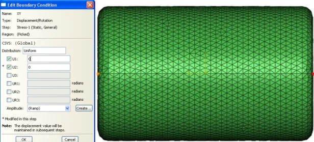
4.3.2.1 Stress analysis step
The user does not participate in the definition of boundary conditions for the stress analysis in Magmasoft. It is an automatic procedure. Therefore we only present our Abaqus approach.
The task is to restrain the rigid body translations and rotations in X, Y and Z, but allow the body to deform naturally (to shrink, basically). In the cylinder model the 6 degrees of freedom has been constrained as follow:
Translations in X, Y and Z
In the flat face of the Cylinder lying in Z=0, a node in Y=0 is constrained in X, Y and Z. See Figure 4.5. Notice that in the picture, X is the horizontal axis, Y the vertical axis, and the Z axis is perpendicular to the paper.
Figure 4.5. Constraining the rigid body translations in X, Y and Z in the Cylinder
Three rigid body translations have been constrained by fixing the point in the space. As a result the part would shrink toward the point. However, the body could still pivot in our fixed node, so now the rotations have to be constrained.
Rotations in the Y and Z axis
A node also lying in Z=0 and Y=0 but in the opposite side of the part with respect to the fixed node is constrained in Y and Z. See Figure 4.6.
Figure 4.6. Constraining the rotations in Y and Z in a single node selection (in red) for the Cylinder model
The constraint in Y avoids the rotation in Z and the constraint in Z avoids the rotation in Y. The reason why the node is left free to move in X is because that is the correct contraction direction toward the totally fixed node.
Cylinder Results
Rotation in the X axis
A node aligned in the Z axis with the totally fixed one (that is with the same X coordinate and Y=0) lying in the opposite flat face of the Cylinder is constrained in X and Y. See Figure 4.7. In this way the displacement of that node can just happen in Z, ensuring that the length axes of the body will remain parallel to the Z axis.
Figure 4.7. Constraining the rotations in X in a single node selection (in red) for the Cylinder model
4.4 Cooling curves
The following results presented in Figure 4.8 were obtained from the central point of the geometry of the whole Cylinder.
Cylinder Results
4.5 Thermal color spectrums
Figure 4.9. Abaqus (top) and Magmasoft (bottom) thermal color spectrums of the last step after shake out of the Cylinder model.
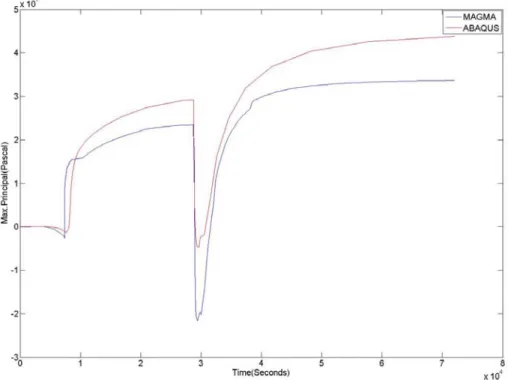
4.6 Stress curves
Figure 4.10. Abaqus vs. Magma Von Mises curves for the Cylinder model
Cylinder Results
Figure 4.12. Abaqus vs. Magma Minimum Principal stresses for the Cylinder model
The stress results presented in Figure 4.10, Figure 4.11 and Figure 4.12 were obtained from the central point of the geometry of the whole Cylinder.
Comments
These results show that the Cylinder model develop more stresses in tension than in compression.
4.7 Stress color spectrums
Figure 4.13. Abaqus (top) and Magmasoft (bottom) color spectrums for the Mises results of the Cylinder model.
Cylinder Results
Figure 4.14. Abaqus (top) and Magmasoft (bottom) color spectrums for the residual
Figure 4.15. Abaqus (top) and Magmasoft (bottom) color spectrums for the residual
Cylinder Results
4.8 Simulation time for the Cylinder
Thermal Stress Total
Abaqus 7hrs. 12min. 24min. 7hrs. 36 min.
5
Original Hub Results
5.1 Geometry
Original Hub Results
Figure 5.2. Bottom view of the Original Hub model
The mold of the original Hub is just a box with the Hub cavity in its center. The external dimensions are 0.7x0.7x0.65. See Figure 5.3.
5.2 Thermal and stress curves points
placement
Figure 5.4. Location of the cooling and stress points of the Hub part
5.3 Mesh
Original Hub Mold
Elements Nodes Elements Nodes
Abaqus 142337 35599 387923 77829
Original Hub Results
Original Hub Results
5.4 Boundary Conditions
5.4.1 Thermal boundary conditions
5.4.1.1 Before Shake-out
Conduction. Between the external surface of the casting and the surface of the mold cavity. For details on how to set this type of boundary condition in Abaqus, refer to section 10.1.1.3.1.1 (under “9-Interaction Properties Definition” and “10-Interactions Definitions”). For details on how to set this boundary condition in Magmasoft, refer to section 10.2.1.3 (instruction for Figure 10.63).
Convection. Between the external surface of the mold and the ambient. For details on how to set this boundary condition in Abaqus, refer to section
10.1.1.3.1.1 (under “10-Interactions Definitions”). In Magmasoft this condition is defined automatically so the user has no participation in the setting.
Radiation. Between the external surface of the mold and the ambient. For details on how to set this boundary condition in Abaqus, refer to section 10.1.1.3.1.1 (under “10-Interactions Definitions”). In Magmasoft this condition is defined automatically so the user has no participation in the setting.
5.4.1.2 After shake out
Convection. Between the external surface of the casting and the ambient. A temperature dependent convective heat transfer coefficient property was defined in Abaqus. For details on how to set this boundary condition in Abaqus, refer to section 10.1.1.3.1.2 (under “9-Interaction Properties Definition” and “10-Interactions Definitions”). In Magmasoft this condition is defined automatically so the user has no participation in the setting.
Radiation. Between the external surface of the casting and the ambient. For details on how to set this boundary condition in Abaqus, refer to section
10.1.1.3.1.2 (under “10-Interactions Definitions”). In Magmasoft this condition is defined automatically so the user has no participation in the setting.
5.4.2 Mechanical boundary conditions
5.4.2.1 Stress analysis step
As mentioned in the Cylinder model results, the user does not participate directly in the definition of boundary conditions for the stress analysis in Magmasoft. It is an automatic procedure. Therefore just the Abaqus approach is presented.
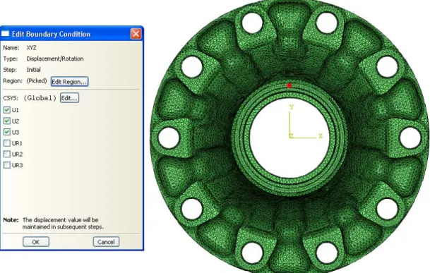
The task is to constrain the rigid body translations and rotations in X, Y and Z, but allow the body to deform. In the Original Hub model the 6 degrees of freedom has been constrained as follow:
Translations in X, Y and Z
In the top flat surface of the Original Hub, a node in X=0 is constrained in X, Y and Z. See Figure 5.7. Notice that in the picture, X is the horizontal axis, Y the vertical axis, and the Z axis is perpendicular to the paper.
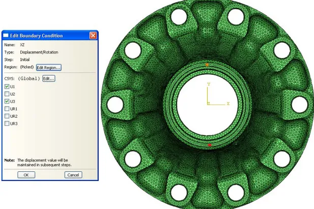
Figure 5.7. Constraining the rigid body translations in X, Y and Z in the Optimized Hub
By fixing this node in the space, three rigid body translations are constrained. Consequently, the part would shrink toward this node. Now, the remaining task is
Original Hub Results
Rotations in the X and Z axis
A node also in the top flat surface of the Original Hub (with the same Z coordinate), and in X=0 is constrained in X, and Z. See Figure 5.8.
Figure 5.8. Constraining the rotations in the X and Z axes in the Original Hub
The constraint in X avoids the rotation in the Z axis and the constraint in Z avoids the rotation in the X axis. Notice that the node is free to move in the Y direction so the part is still able to deform normally.
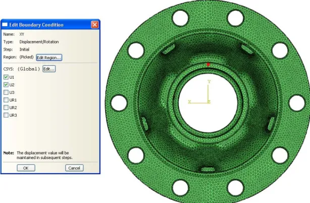
Rotation in the Y axis
A node in X=0 and vertically aligned with the totally fixed node (same Y
coordinate) but in a different Z coordinate, in this case in the flat surface of the end of the cylindrical section of the hub, is constrained in X and Y. See Figure 5.9. In this way the rotation in the X axis is restrained and all vertical axes of the part are fixed to remain parallel to the Z axes.
Original Hub Results
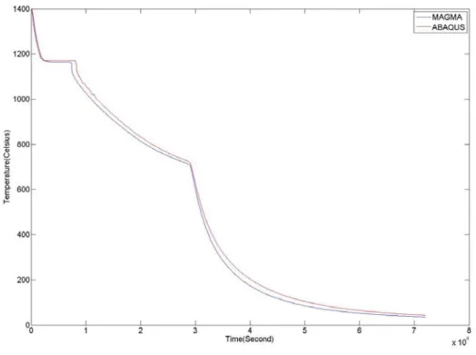
5.5 Cooling curves for the Original Hub
Figure 5.10. Abaqus vs. Magmasoft cooling curves for the Hub model
The results presented in Figure 5.10 were obtained from PNT0 which location is shown is Figure 5.4.
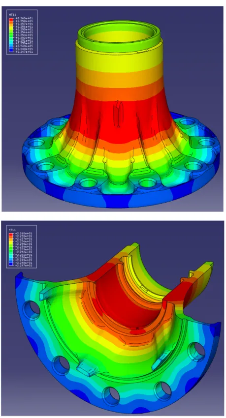
5.6 Thermal color spectrums
Figure 5.11. Abaqus thermal color spectrums for the last step after shake-out of the Original Hub model
Original Hub Results
Figure 5.12. Magmasoft thermal color spectrums for the last step after shake-out of the Original Hub model
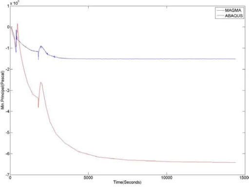
5.7 Stress curves for the Original Hub
Using PNT0 as reference point as shown in Figure 5.4: