HALMSTAD
UNIVERSITY
Master's Programme in Embedded and Intelligent
Systems, 120 credits
Modelling behaviour of Agents using a
Particle Filter based Approach
Computer science and engineering, 30
credits
Halmstad 2019-09-01
Sheikha Al-Azri
__________________________________
School of Information Science, Computer and Electrical Engineering Halmstad University
PO Box 823, SE-301 18 HALMSTAD Sweden
Master Thesis
Embedded and Intelligent Systems
2019
Author: Sheikha Sulaiman Al-Azri
Supervisor:
Dr. Björn Åstrand and
Naveed Muhammed
Examiner: Slawomir Nowaczyk
Modelling Behaviour of Agents using a Particle Filter based Approach Sheikha Al-Azri
© Copyright Name(s) of author(s), 2019. All rights reserved. Master thesis report IDE 12XX
School of Information Science, Computer science and Engineering Halmstad University
i
Abstract
Continuous development in the field of Artificial Intelligence (AI) is expanding the replacement of manually driven vehicles by Intelligent Vehicles (IV). One of the most important aspects of automated vehicles in real-world practice is safe driving with zero chance of an accident. In this thesis, we propose a method based on a Particle Filtering algorithm, with 1000 particles, to model the behaviour of other agents and predict the intention and future position for long-term and short-term prediction.
The approach was implemented to model the behaviour of other agents around an autonomous vehicle based on a set of trajectories (reference trajectories) navigated by those agents. Furthermore, we have tested and presented the results of the algorithms on the Edinburgh Informatics Forum dataset for pedestrian and the MIT trajectories data sets, with multiple camera views for modelling vehicle behaviours. The behaviour was modelled according to some features (attributes) extracted for each reference trajectory including angles, position and velocity. The study found that the developed algorithm could be applied for a wide range of data that was supplemented with trajectory data defined by position and time. In addition, the algorithm showed the ability to perform excellently in multi-class problems. This approach has been applied for recognizing and predicting the intention of two different types of agents, pedestrians and vehicles, moving through different trajectories in different scenarios. The results showed that the angle feature indicates the best accuracy in the early stage (up to 90%). The results further revealed that the quality of the set of reference trajectories, which were used to model the behaviour, had a significant role in the accuracy of the model. The algorithm was able to model the behaviour using a small set of reference trajectories, however as the number of the trajectories increased, the better the accuracy of the results. Increasing the number of reference trajectories has given us a chance to increase variability on the results. This can be attributed to some reference trajectories being of poor quality due to overlapping paths or the presence of outliers. This method allowed us to limit computational complexity due to the fundamental of data representations and the related operation used to manipulate them.
ii
Acknowledgment
I would like to express our sincere gratitude to supervisors, Dr. Björn Åstrand and Naveed Muhammad, who not only served as our research supervisors, but were also sources of inspiration. I would like to thank them for their continuous encouragement, guidance and support throughout our thesis journey. I greatly appreciate their valuable assistance.
My deepest thanks go to my husband, for shouldering the responsibilities of home and children, which gave me the time to complete this work.
I would like to extend our appreciation to all present and former colleagues for their continued support, guidance and collaboration
Contents
Abstract ... i
Acknowledgment ... ii
1 Introduction………1
1.1 Problem definition ... 1 1.2 Contribution ... 1 1.3 Related Work ... 2 1.3.1 A safety environment ... 21.3.2 Modelling the behaviour ... 3
1.3.3 Particle filter approach: ... 3
2
Methods ... 9
2.1 Particle filter structure ... 9
2.1.1 Inserting Data:... 10
2.1.2 K-fold cross validation:... 14
2.1.3 Feature Extraction: ... 14
2.1.4 Applying PF classifier method: ... 15
2.1.4.1 Initialization of particles: ... 16
2.1.4.2 Measurement update: ... 16
2.1.4.3 Resampling update: ... 17
3
Rational of algorithm development ... 21
3.1 Implementation of the algorithm ...21
3.1.1 Using angles as only feature ... 24
3.1.2 Using position as a feature: ... 29
3.1.3 Using velocity as a feature: ... 34
3.1.4 Using position and angle as features: ... 37
3.1.5 Using position, angle and velocity features: ... 39
4
Results ... 43
4.1 The algorithm (PF) recognition results: ...43
4.1.1 Angle feature: ... 44
4.1.2 Position Feature: ... 47
4.1.3 Velocity feature: ... 50
4.1.4 Position and Angle features: ... 53
4.1.5 Position, Angle and velocity features: ... 55
4.2 Predicting future Position for short-term and long-term: ...57
5
Discussion ... 61
5.1 Number of reference trajectories ...61
5.2 Data sets used ...62
5.3 Features used ...63
5.4 Prediction of future state ...64
5.5 Suitability of using PF approach ...66
List of Figures
Figure 1: Model Overview... 9
Figure 2: A view of the scene and image data from which the detected targets “Edinburgh Informatics Forum Pedestrian” ... 10
Figure 3: (a) All tracked trajectories from dataset 28Aug and (b) The extracter tracked trajectories in the dataset 28Aug. ... 11
Figure 4: Raw trajectories used for testing and training. ... 11
Figure 5: Spline trajectories categorized three classes. ... 12
Figure 6: (a) MIT Trajectory Camera 1 view. (b) Plotting all the trajectories from that Camera. ... 13
Figure 7: Vehicles trajectories after categorized into two cats. ... 13
Figure 8: Vehicles spline trajectories categorized cat.1 red color and cat2. blue color. ... 14
Figure 9: Flowchart PF algorithm. ... 16
Figure 10: Average reference trajectories (pedestrian). ... 19
Figure 11: Average reference trajectories (Vehicles). ... 19
Figure 12: Predicting the vehicle’s position after a second ahead. ... 20
Figure 13: Predicting vehicle’s position after 5 seconds ahead. ... 20
Figure 14: Test spline Trajectory “pedestrian”. ... 22
Figure 15: Reference spline trajectories used as training trajectories “pedestrians”. . 22
Figure 16: Test spline Trajectory “Vehicle”... 23
Figure 17: Reference spline trajectories used as training trajectories “MIT dataset”. . 23
Figure 18: State Evolution for the belief of PF about the observed Agent for belonging to one of the three categories (Angle feature-pedestrians) ... 25
Figure 19: Angles features for all the reference Trajectories ... 25
Figure 20: Angles for all the reference Trajectories (vehicles). ... 27
Figure 21: State Evolution for observed Agent for belong to one from the two categories (Angle feature- vehicles). ... 28
Figure 22: Short-term (1 sec) and Long-term (5 sec) Predicting position using angles features (pedestrian). ... 28
Figure 23: Predicting position Short (1 sec) and long-term (5sec) using angles features (vehicle). ... 29
Figure 24: Map position features for all the reference Trajectories (Pedestrians). ... 31
Figure 25: State Evolution for observed Agent (Position feature- Pedestrians). ... 32
Figure 26: Short-term (1 sec) and Long-term (5 sec) Predicting position using position features (pedestrian) ... 32
Figure 27: Map position features for all the reference Trajectories (vehicles) ... 33
Figure 28: State Evolution for observed Agent (Position feature- vehicle). ... 33
Figure 29: Short-term (1sec) and Long-term (5 sec) Predicting position using position features (vehicle). ... 34
Figure 30: Map velocity features for all the reference Trajectories (Pedestrians). ... 35
Figure 31: State Evolution for observed Agent (velocity feature- pedestrian). ... 35
Figure 34: Short-term (1 sec) and Long-term (5 sec) Predicting position using velocity features (pedestrian). ... 37 Figure 35: Short-term (1 sec) and Long-term (5 sec) Predicting position using velocity features (vehicle). ... 37 Figure 36: State Evolution for observed Agent (pos-angle features- pedestrian). ... 38 Figure 37: Short-term and long-term prediction using pos-angle features
(pedestrian). ... 38 Figure 38: State Evolution for observed Agent (pos-angle features- vehicle). ... 39 Figure 39: Short-term and long-term prediction using pos-ang features (vehicle). .... 39 Figure 40: State Evolution for observed Agent (pos- angle-velocity features-
pedestrian). ... 40 Figure 41: Short- and long-term prediction using pos-angle-velocity features
(pedestrian). ... 40 Figure 42: State Evolution for observed Agent (pos- angle-velocity features- vehicle). ... 41 Figure 43: Short- and long-term prediction using pos-angle-velocity features
(vehicle). ... 41 Figure 44: An example of a percentage of samples to a test trajectory (pedestrian and vehicle) . ... 43 Figure 45: Early stage for two dataset pedestrians and vehicles. ... 44 Figure 46: A percentage for early stage10% to 40% for both datasets... 44 Figure 47: Boxplot accuracy vehicles and pedestrians using angles features 2-fold for all percentages of samples ... 46 Figure 48: Boxplot accuracy vehicles and pedestrians using angles features 5-fold for all percentages of samples ... 46 Figure 49: Average accuracy 5-fold and 2-fold using angle features for pedestrian and vehicles. ... 47 Figure 50: Boxplot accuracy (vehicles) using position features 2-fold and 5-fold for all percentages of samples. ... 49 Figure 51: Boxplot accuracy (pedestrians) using position features 2-fold and 5-fold for all percentages of samples ... 49 Figure 52: Average accuracy 5-fold and 2-fold using position features for pedestrians and vehicles. ... 50 Figure 53: Boxplot accuracy (pedestrian) using velocity features 2-fold and 5-fold for all percentages of samples. ... 52 Figure 54: Average accuracy 5-fold and 2-fold using velocity features for vehicles and pedestrians... 52 Figure 55: Average accuracy 5-fold and 2-fold using velocity features for pedestrians and vehicles. ... 52 Figure 56: Boxplot accuracy (pedestrians) using pos-angle features 2-fold and 5-fold for all percentages of samples ... 54 Figure 57: Boxplot accuracy (vehicles) using pos-angles features 2-fold and 5-fold for all percentages of samples ... 54 Figure 58: Average accuracy 5-fold and 2-fold using pos-angles features for
pedestrians and vehicles. ... 55 Figure 59: Boxplot accuracy (pedestrian) using Pos-Angle-velocity features 2-fold and 5-fold for all percentages of samples... 56
Figure 61: Average accuracy 5-fold and 2-fold using pos-angle-velocity features for pedestrians and vehicles. ... 57 Figure 62: Predicting position short-long term using angles only for both datasets. . 58 Figure 63: Predicting position short-long term using position only for both datasets. ... 58 Figure 64: Predicting position short-long term using pos-angles only for both
datasets. ... 59 Figure 65: Average Accuracy to all features for recognizing the category used by the algorithm for both datasets. ... 64 Figure 66: A comparison results of average error of short-term and long-term
prediction on pedestrian for all features (angles, position and pos-angles). ... 65 Figure 67: A comparison results of average error of short-term and long-term
List of Tables
Table 1: A classification result for observed trajectory from starting point to the goal (pedestrians) ... 24 Table 2: A classification result using angles features for observed trajectory (Vehicles) from starting point to the goal. ... 27 Table 3: A classification result using position features for observed trajectory
(Pedestrian) from starting point to the goal. ... 31 Table 4: A classification result using position features for observed trajectory
(Vehicle) from starting point to the goal. ... 33 Table 5: A classification result using velocity features for observed trajectory
(pedestrian) from starting point to the goal. ... 35 Table 6: A classification result using velocity features for observed trajectory
(vehicle) from starting point to the goal. ... 36 Table 7: A classification result using pos-angle features for observed trajectory
(vehicle) from starting point to the goal. ... 38 Table 8: A classification result using pos-angle features for observed trajectory
(vehicle) from starting point to the goal. ... 39 Table 9: A classification result using pos-angle-velocity features for observed
trajectory (pedestrian) from starting point to the goal. ... 40 Table 10: A classification result using pos-angle-velocity features for observed
trajectory (vehicle) from starting point to the goal. ... 41 Table 11: Average accuracy and variance using angles 5-fold for all percentages of samples (Pedestrian). ... 45 Table 12: Average accuracy and variance using angles features 2-fold for all
percentages of samples (Pedestrian). ... 45 Table 13: Average accuracy and variance using angles 5-fold for all percentages of samples (vehicles). ... 45 Table 14: Average accuracy and variance using angles 2-fold for all percentages of samples (vehicles). ... 45 Table 15: Average accuracy and variance using position 5-fold for all percentages of samples (pedestrians)... 48 Table 16: Average accuracy and variance using position 2-fold for all percentages of samples (pedestrians)... 48 Table 17: Average accuracy and variance using position 5-fold for all percentages of samples (vehicles). ... 48 Table 18: Average accuracy and variance using position 2-fold for all percentages of samples (vehicles). ... 48 Table 19: Average accuracy and variance using velocity 5-fold for all percentages of samples (pedestrian). ... 50 Table 20: Average accuracy and variance using velocity 2-fold for all percentages of samples (pedestrians)... 51 Table 21: Average accuracy and variance using velocity 5-fold for all percentages of samples (vehicles). ... 51
Table 23: Average accuracy and variance using pos-angles 5-fold for all percentages of samples (pedestrians). ... 53 Table 24: Average accuracy and variance using pos- angles 2-fold for all percentages of samples (pedestrians). ... 53 Table 25: Average accuracy and variance using pos-angles 5-fold for all percentages of samples (vehicles). ... 53 Table 26: Average accuracy and variance using pos-angles 2-fold for all percentages of samples (vehicles). ... 54 Table 27: Average accuracy and variance using pos-angle-velocity 5-fold for all percentages of samples (pedestrians). ... 55 Table 28: Average accuracy and variance using pos-angle-velocity 2-fold for all percentages of samples (pedestrians). ... 56 Table 29: Average accuracy and variance using pos-angle-velocity 5-fold for all percentages of samples (vehicles). ... 56 Table 30: Average accuracy and variance using pos-angle-velocity 2-fold for all percentages of samples (vehicles). ... 56
1 Introduction
Extensive research in mobile robotics has brought a revolutionary change in the industrial field. Due to more flexibility, robustness and efficiency, Automated Guided Vehicles (AGVs) are playing a significant role in manufacturing industries. AGVs are normally operated on predefined and fixed pathways, which contain guidewires embedded inside the floor, or reflective strips on a floor and are guided by sensors mounted on the AGVs. The actions of AGVs in the warehouse environment depend on the other agents in the environment. Because of this Multi-Agent co-ordination [1], safety in warehouses has become a significant issue. While working in a warehouse environment, AGVs should not harm other agents, objects in the environment, and the AGVs themselves.
1.1 Problem definition
The main purpose of this project is to develop a safety system in industrial vehicles, especially autonomous vehicles like Automated Guided Vehicles (AGVs), in the warehouse environment. Most of the current safety systems are based on control systems [2], onboard sensors (such as lidar, radar and cameras), Vehicle to Vehicle and Vehicle to Infrastructure communication [3]. A number of onboard sensors have been integrated into the robots and the environment and can detect obstacles for collision avoidance. One of the main drawbacks with these sensor systems is that their functionality is restricted to line-of-sight conditions. These sensors find an obstacle at a short distance from them, especially at junctions, and the chance of collision increases in this scenario. Recent studies have improved this to some extent, by providing Vehicle to Vehicle and Vehicle to Infrastructure wireless communications.
More studies have been conducted in this field and have shown improvement in decreasing the number of accidents [4], however further investigations are needed to increase safety with a minimal chance of accidents. Today’s safety systems do not incorporate the behaviour of different agents in the surrounding environment. To overcome the limitations in today’s safety systems, we focus on modelling the behaviour of the other agents.
The goal of this project is to build a method, to model the behaviour of agents based on reference trajectories and evaluate the accuracy of the method to recognize and classify the behaviour. Furthermore, the method aimed to utilize the behaviour to predict the next position of the corresponding agent in time (after an interval of a matter of seconds).
We have modelled the behaviour of an agent and predicted the intention of an agent and the agent’s position a few seconds ahead, by implementing Particle Filter. Particle Filter is a developing method used for Autonomic vehicles and presents an agent-based simulation of vehicles and pedestrians to model their behaviour in environments such as a warehouse, wherein multi-agents are situated. The method is based on using a set of reference trajectories. The extracted features from the reference trajectories were treated by particle filter to find the matching one in the behaviour. The proposed approach was applied in two publicly available databases: the Edinburgh Informatics Forum pedestrian dataset [5] and the MIT trajectories data set, with multiple camera views[6] to model the vehicle’s behaviours. The method can be applied to improve the performance of an autonomous vehicle’s decision-making in crowds such as AGVs in a warehouse environment.
1.3 Related Work
Many studies using various approaches and techniques have been reported in the development of autonomous vehicle safety. In the next section, a brief description about the development of safety approaches for AGVs and the relevant approaches that have been used.
A safety environment
The central issue for an autonomous vehicle is safety. As mentioned earlier, our project will focus on developing a safety system for automated vehicles that have to operate and populate with other agents like AGVs in a warehouse. Safety always needs to be fully addressed when sharing operational activities with humans in the same environment. A human is required to cooperate and interact with AGVs in a warehouse environment to assign it some task. Thus, user-friendly interfaces integrated with AVGs were developed as previously programmed [7], [8]. But in these interfaces, the behaviour of the human is unpredictable and cannot interact to avoid obstacles. For these reasons, sensors are used [9] like bumpers or laser scanners to avoid the obstacles. However, these types of equipment on AGV systems are limited, as they are not able to react with different kinds of obstacles in a specific manner. However, the AGVs should consider the behaviour or the identity of different agents around them to increase safety.
In this case, we need the environment to be free from accidents, so it is important to provide autonomous vehicles with a control system able to assess an environmental threat. A threat assessment algorithm [10] was developed and used to predict the future movement of other vehicles. This has led to propose an algorithm that can accurately detect driver intentions and prevent motion predictions using a random forest classifier. In addition, the algorithm computes possible future trajectories after recognizing the driver intention using a particle filter.
us to focus on methods that enable the system to be more flexible in order to predict the future trajectory. Our real-world system is non-linear, so we need stochastic motion prediction methods for state estimation and prediction of the vehicle , such as the Extended Kalman Filter (EKF), the unscented Kalman Filter (UKF), and the Particle Filter (PF) [11]–[13].
The challenge is to understand the situation of the environment from perception sensors and detecting the objects at intersections. This can potentially be solved using cooperative communication technology [14]. This system provides early advisory warnings to reduce traffic conflicts. But there is a lack of information about the driver’s future actions for early and reliable intersection assistance. The decisions concerning which objects must be considered as relevant and which must not, are highly dependent on the future trajectory.
Predicting the driver intention is a significant issue for obstacle avoidance. Predicting the driver’s turn intention at urban intersections is presented in the literature [15]. The novelty in that work was to implement a context-based prediction of the future driving maneuver that warns the driver several seconds before the driving trajectory changes. They successfully give an example showing the need for turn intention systems to predict driver maneuvers for right turns, left turns or straight driving. The advantages of this system are the ability to predict intentions earlier than by using physical changes in a vehicle’s trajectory (i.e. steering wheel angle or yaw rate) and the functionality for different types of intersections, thus, it is suitable for many different types of intersections in real driving conditions. This approach is not applicable to straight drives, but it works fine for turn maneuvers.
Modelling the behaviour
Many approaches were proposed for modeling the behaviour of driver in artificial potential field. One of these approaches proposed by Khatib [16], considered multiple hypotheses with respect to the driver’s intentions. They created several force fields used for modelling driver behaviour and these fields partially overlap each other making a complex force field. This was implemented and evaluated by a prototype that consisted of two units (road-side unit with HMI touch screen and on-board antenna unit placed in a vehicle). The system monitored driver behaviour and broadcast a warning message if the driver behaved abnormally, for example not stopping at a red light. Warnings were used as an indicator of unpredicted driver behaviour by comparing the likely behaviour from the history of driver intentions. A driver behaviour model was proposed to warn the driver and increase their prediction behaviour in such traffic rules and driver intention called a cooperative warning system [17]. By creating a number of force fields in lane following, and red-light braking behaviour. They chose a pedestrian crossing scenario to test their warning system by comparing driver behaviour with a set of expected reference behaviours. The warning is generated by observing the force vector after a given
of applicable intentions.
Some studies based on machine learning techniques have been used for agent or driver intention estimation. For example paper [18] estimates the intention for a car-following maneuver using three techniques of machine learning; Support vector Machine (SVM), Neural Network (NN) and Hidden Markov Model (HMM). Driver intention estimation and predicting the path in lane-change scenario based on SVM, is presented in [19]. Also SVM has been used in paper [20] with the aim of predicting vehicle behaviour. Another approach based on (HMM) was proposed for estimating and recognizing driver intentions by identifying the hidden driver states [21], [22]. In addition, HMM was used to estimate and predict the driver states at an intersection [23]. In that study, the combination of HMM with a hybrid state system architecture was addressed to achieve a maximum level of safety. Paper [24] focuses on observing the driver behaviour and vehicle state if the states under normal or dangerous driving behaviour, predicting the future trajectory of a lane changing, and classifying the model based on Hidden Markov Models (HMMs).
Hidden Markov Models have been widely using in facial recognition proposed in [25], and speech recognition, especially with time-sequential data. Then it was introduced into the robotic field to learn the motion patterns of people [26], HMMs are one of the first machine learning techniques used to predict motion pattern. They used an Expectation Maximization (EM) algorithm, to cluster the trajectories into a motion pattern and then used them to feed HMMs, and used HMMs to maintain a belief about the positions of persons.
Paper [27] used HMM for pattern recognition, to predict driver intensions such as lane changes or staying in the lane. As parameters, they used transition probabilities, an emission matrix and the initial state distribution[28]. They implemented individual HMMs for each event (right, left and straight). And then classified the observation based on the calculated observational likelihoods for all the models. In [29] a single HMM was constructed instead of constructing individual models for each event to estimate the parameters easily. They estimated the parameters for the model by using a training set and validated the model by using a test set. They constructed an HMM based on the idea, that they assumed 3 events Left turn (LT), Right turn (RT) and Straight Forward (SF) as 3 hidden states and observation sequence was modelled by emission matrix.
A method for detecting steering events such as curves and maneuvering was proposed using hidden Markov models (HMMs) based on vehicle logging data [29]. They considered three steering events as hidden states (right turn, left turn and straight forward) and constructed the HMM model based on them. The results from the classification indicate that methods can recognize left and right turns with small misclassification errors.
Many studies have also made extensive use of probabilistic techniques that learn parameters from large training data [30][31]. Another approach [32] presents a new
direct applications in automated video surveillance. They used an extension of the Rao-Blackwellised Particle Filter (RBPF) as an efficient inference mechanism, in which the result classification accuracy compared against a trained Hidden Markov Model and Particle Filter (PF). This showed that their approach achieves a 92% accuracy at video frame rate. Furthermore, [33] [34] showed that the RBPF gives more accurate estimates than a standard Particle Filter and is more efficient than a Bayesian Filter. Moreover, some approaches use PF for detecting the abnormal behaviour of moving objects [35].
Based on the PF’s special advantage in tracking and predicting linear, non-Gaussian moving objects, we used it for modelling an object’s behaviour of moving objects. The following section will explain the background of this method.
Particle filter approach:
The basic principle of the PF approach is estimating the state by a large random samples or particles. These particles are a stochastic distributed in the state vector. Then, these particles are propagated and updated with new measurement in principle of corrector cycle. After that, a resampling step is required to keep the particle with highest weight [36]. There are many ways of doing the resampling step, however a “systematic resampling algorithm” [37] was used in this work. This technique can result in a phenomenon known as degeneracy, which can be solved using an approached called Interactive Multiple model [38], allowing us to control the number of particles in order to avoid degeneracy when the mode changes.
At first, successes of implementation using the particle filter method can be found in the area of robotics localization [39][40]. Many recently fielded studies about robotic systems employ probabilistic techniques for perception [41], [42], and some using probabilistic techniques at levels of perception and decision making [43]. In this work, we don’t use PF for localization, instead we used it to model the behaviour according to a set of reference trajectories.
PF has been used as an estimation technique based the principle of recursive Bayesian estimation. PF has been shown to be effective in dealing with tracking problems. It provides suboptimal solutions to the recursive Bayesian approach [44].
Modelling the behaviour is not simple as a single dynamic model. It is common as a nonlinear problem, which can be solved by an extended Kalman Filter and Particle Filter [45]. The Particle Filter has almost complete generality to any non-linearity and any distributions. In addition, it provides a good accuracy in predicting and it is flexible in addressing data prediction problems. As mentioned in reference [37], a particle filter approach was developed for real-time prediction using a real time and historical data set. That research also used a partial resampling strategy for solving a degeneracy problem by replacing low weighted particles with historical data. Each particle can produce a travel time prediction value according to the similarity of traffic patterns between each particle and time traffic measurement.
the driver’s intensions early. Vehicle’s speed is a significant feature to estimate the driver’s intent, when it approaches towards junctions. If the velocity of the vehicle seems to slow down it might be a turning behaviour (right or left), rather than car-fallowing behaviour [33], [46]. An Intelligent Driver Model [38] can be used to represent both car following and turning behaviours. Instead of the machine learning approach, where patterns of observed behaviour are used to estimate future behaviour, proactive vehicle alert system [46] proposes explicit models, which can later be compared with observations. The behaviour of vehicle was modelled by developing the state vectors i, recursively at time k as shown in equation (1).
, (1)
Where, d is distance from the starting, v is velocity, and p is path intended. By using current state vectors, calculating the most likely value of state vector, driver intensions in the next time step recursively, and then comparing which evolutions closely matched to the observed measurements. State vector in the next step is given by [46], in equation (2):
, (2)
Where, f(x) in (2) is the process model, T is the sampling interval, and ϕk is zero mean
Gaussian noise. g(𝑥𝑘𝑖, 𝑌k) is speed evolution, which depends on the present vehicle state
and the observations of all other vehicles (𝑌k) at time k.
, (3)
In equation (3) ωk refers to zero, meaning Gaussian noise, and h (𝑝𝑘𝑖) is the link of the
path up to and including the current one.
The driver’s intention was estimated using a computational particle filter, which limited the approach to non-real time use. Similar to the approach in [46], paper [3] introduced a method to infer the driver’s intent for urban intersections based on a Bayes net instead of a particle filter and real time capable approach. They used an Intelligent Driver Model (IDM) to model the driver behaviour for car-following, the model (IDM) is given in (4):
, (4)
Where in equation (4) samples: ˙v in a parameter for acceleration, a maximum acceleration parameter, v the current actual velocity, u the desired velocity and δ a fixed acceleration exponent. The influence of a vehicle is represented by the ratio of the desired gap d∗ and the actual gap d. The parameter sets can be used as hypothesis
H for the actual driver behaviour in an unknown situation. Then, a simple Bayes net
model used for driver intent inference based on I actual driver intention, H hypothesis and O observation given in (5):
(5)
This paper achieved a good classification performance and an advantage of this approach that, if the driver cannot be inferred in a particular situation, it can be easily extended to include additional features such as turn indicator or lateral displacement. Similar to the approach taken in [46], we are going to introduce a method to infer agent intent, based on an explicit model for the modelling the behaviour using a set of reference trajectories. This model is more transparent than machine learning methods and more robust when generalized to situations to observe behaviour. This serves to predict future positions and allows for specifying rare behaviours as well as allowing us to model and predict the next position based on similarity of behaviours in traffic laws.
We are focusing on comparing the trajectory with the similar agent behaviour obtained from different reference trajectory sets and estimating their posterior probabilities in a manner similar to [46]. The result of the probability distribution can be used to make predictions about future trajectory. But they are comparing the trajectory of the past few seconds with the simulated driver behaviour obtained from different parameter sets. Instead, we will use datasets as historical data that enables us to categorize the behaviour of the observed agent according to a similar one from these available data (references trajectories). Another method added to our algorithm after recognizing the category of the agent, which used to predict where the agent will be in next step after seconds ahead as long and short-term prediction. The prediction step comes after recognizing the category of the agent then the prediction is done by taking the average of all reference trajectories in each class and predicting the next position based on the selected class. Long and short-term prediction of objects (agents) motion is an important task for applications such as robot navigation in a crowded environment [47]. In particular, predicting a future position for surrounding agents over shorter and longer periods significantly improves the robot’s decision making and avoids collisions on its planned trajectory. As we know in general that PF has widely been used to estimate the motion of objects using their trajectories and
They proposed a trajectory predictor to learn prior knowledge from annotated trajectories and transferred it to predict the motion of the target object. Then, they used convolutional neural networks to extract the visual features of target objects used for long and short-term prediction. This method predicts the trajectory based on sequential tracked features, sequential location information of the target object and possibly also the prior trajectory knowledge.
The interest of the international scientific community is moving towards video surveillance systems implementing real-time automatic object-behaviour analysis. This work focuses on analyzing and understanding different kinds of moving objects (pedestrians and vehicles) from public datasets. The Edinburgh Informatics forum pedestrian dataset [5] has been implemented to a publicly available video database and provides a comprehensive set of trajectories of walkers computed from a fixed overhead camera 23 meters from the ground. The dataset has been used in the robotics field to demonstrate surveillance algorithms, especially for detecting behaviours; see [50] ,[51] ,[52] and [53]. Generally, in this work we are presenting a method for modelling the behaviour using the PF to model the behaviour of pedestrian agents by using the same database from the Edinburgh Forum. Furthermore, for modelling the behaviour of vehicles, we are going to use the MIT trajectory data set [6], available for research analysis in multiple single camera views using the trajectories of objects. More details about the data and its implementation are explained in Chapter 2, section 2.1.1. To the best of our knowledge, the algorithm has not been used for modelling the behaviour on the same technique on same datasets.
The thesis is structured as follows. Chapter 2 describes the methodology for behaviour modelling as well as predicting the future state (position) using the PF method. Chapter 3 illustrates the results from the classification methods and prediction. Chapter 4 presents the discussion based on the reviews. Finally, a summary of this thesis is presented in chapter 5.
Chapter 2
2 Methods
2.1 Particle filter structure
In this thesis, the particle filter used as a method for modelling the behaviour instead of using it for localization [54]. Similar to the approach in paper [46], the particle filter model implements for predicting path choice and driver intention. Mainly, the behaviour of the agent is modelled by developing the state vectors recursively. Hence by observing the agent’s position, the agent’s speed and the agent’s orientation this is extracted from the state of agent by processing the raw data.
So here we propose an overview for the particle filter model as illustrated in Figure 1: Error! Reference source not found.
Inserting Data
Feature Extraction
Applying PF classifier method
Predicting future state
Inserting Data:
The algorithm was trained and tested on a publicly available dataset consisting of a set of trajectories of detected targets of people walking through the Edinburgh Informatics Forum [5]. There are about 1000 trajectories for each working day in the dataset. Figure 2 shows a view of the scene and image data from which the detected targets are found. The camera is fixed overhead approximately 23 m above the floor. The images size is 640x480 pixels in which each pixel horizontally and vertically corresponds to 24.7 mm on the ground.
The implementation of the algorithm was tested using the observation recorded on August 28th, "tracks. Aug28" file as shown in Figure 3 (a). In addition to the track file, which contains position information (x, y, t), spline file "spline. Aug28" was used. The later file provides the average error of the spline fit to the tracked trajectories as well as the control points. The spline fitting algorithm and its implementation is provided by Rowland R. Sillito[55]. Moreover, normalization has been applied in the main file since the spline fit works only on a variable between 0 and 1. As a result, the X and Y values were multiplied by 640 and 480 respectively to get the real values in the photo size before they were used in our work.
Using the control points, all trajectories were approximated by cubic spline curves, this was done by using the B-spline method [68] that interpolated the 6th control points
in the spline file per each trajectory. This approximated to choosing trajectories to an equal number of size 50 points in each trajectory with a non- uniform distribution. However, our algorithm was tested with several more points but the one with 50 gave us satisfying results. Using Spline curves helped the algorithm determine the curve points and was well suited for implementation.
Figure 2: A view of the scene and image data from which the detected targets “Edinburgh
In order to have more specific paths, we cleared the data and extracted the trajectories
that give visible, clear paths and destinations. Figure 3 (b) shows the plot of trajectories that we extracted from the data file titled August 28th. We have chosen three different goals and paths as references, which allowed the algorithm to be able to categorise the test trajectories. Then, we picked up 90 suitable trajectories by specifying the end points for each category, by eliminating all the unobvious trajectories that would not lead to a clear goal as shown in Figure 4.
Where,
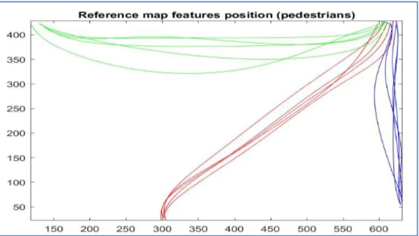
Figure 5 illustrates after implementing the spline curves to the selected trajectories. The number of reference trajectories classified into three categories is given different colours, the red colour despite the trajectories belongs to category 1, green colour for category 2 and blue colour for category 3.(a) (b)
Figure 3: (a) All tracked trajectories from dataset 28Aug and (b) The extracter tracked trajectories in the dataset 28Aug.
Reference trajectories were used to model the behaviour. Those selected references can be acceptable from any number of different trajectories and be comprised equally in each category. These categories are the classes that our algorithm should classify the behaviour of test data into them.
Since this thesis focuses on the warehouse environment, we need to model the behaviour of different types of agents in a warehouse where there are different kinds of autonomous vehicles and manually driven vehicles. So, another data set used for training and testing the algorithm is the MIT trajectory data set with multiple camera views [6] to model the behaviour of the vehicles instead of pedestrians. This public data set allows for the research of activity analysis in multiple single camera view using the trajectories of objects as features. In total, are four camera views comprising both traffic and predictions. Each camera view is sized 320 x 240 pixels and each camera view is quantized into 64x48 cells. More details about the scene ground plane of the camera were obtained from the previous work [56]. They calculated the scene ground plane of the camera view manually using a metric reflection homograph with a direct Linear transform algorithm (DLT) [57]. The camera view covers 1200 x 850 m in the ground and its associated masks have a resolution of 0.4 m/pixel.
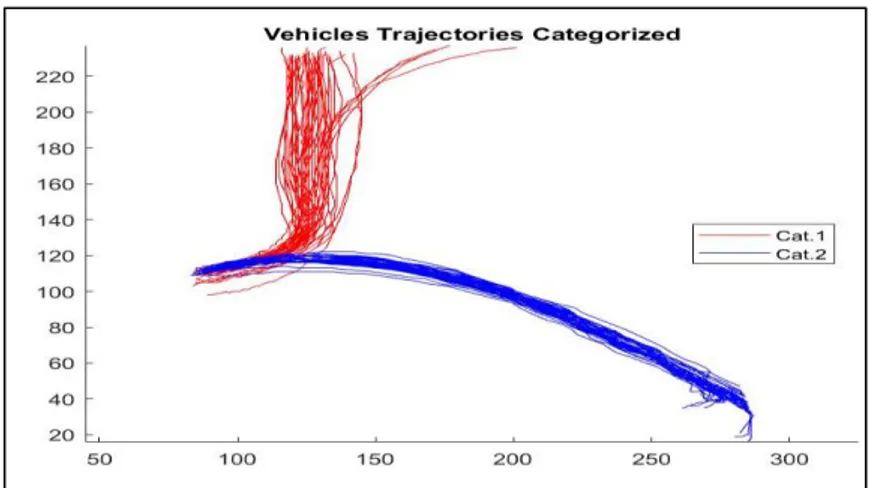
In this thesis, we used the data set extracted from camera 1 (MIT trajectories data set) as shown in Figure 6 (a), where Figure 6 (b) shows the plotted of all trajectories that were recorded from the camera view which included pedestrians and vehicles. We tested and trained the developed algorithm and only used the trajectories belonging to vehicles, as shown in Figure 7. Figure 8 illustrates the selected trajectories of vehicles after implementing the spline curves.
1.Cat1 ___
2.Cat2 ___
3.Cat3 ___
(a) (b)
Figure 6: (a) MIT Trajectory Camera 1 view. (b) Plotting all the trajectories from that Camera.
K-fold cross validation:
Cross-validation is a commonly employed technique used to evaluate classifier performance over a dataset [58]. One type of cross validation is the K-fold procedure, which was used to evaluate the algorithm in this study. In K-fold cross validation the dataset randomly patrician into K subsamples. This process can repeat K times and each K subsamples for the test data used exactly one time is not used again as a test. To evaluate the algorithm, we used the K-fold cross-validation method, which allowed us to verify the performance of the PF classifier model. In this procedure we used different parameters called K that refer to the number of groups that split the data into equal numbers of the data set, where the data were divided into training and testing sets. The total dataset used 60 trajectories as pedestrians from the “Edinburgh data set” and 100 trajectories as cars from the “MIT trajectories data set”. These trajectories will be divided into K groups where K= 2 and K= 5. They have equal numbers of trajectories from each category. One of these K groups will be used to test the classifier and the other was used to train the algorithm with the remaining K−1 groups. All samples were used in the validation either as test or training sets.
Feature Extraction:
For each and every selected trajectory we extracted the behaviour of the agents. The features of reference trajectories were obtained this way. These features are angles, position and velocity. We use a feature’s function similar to the one used in [59] for capturing the trajectory properties. After that, we used them by the PF to classify the test trajectory and according to the similarities between the feature of the observed trajectory and the features for the reference trajectories. Further explanation about the features is given below:
• Position:
Figure 8:Vehicles spline trajectories categorized cat.1 red color and cat2. blue color.
trajectories and the test trajectory. • Velocity:
The agent velocity is necessary and can be extracted from the position information and time of the real trajectory. We simply calculated the displacement by the agent and divided the value for each step by the time that the movement takes. Displacement is computed using Euclidean distance for each two consecutive points.
Since we are using spline line trajectories, we don’t have velocity and time values. To solve this problem, we assigned values (velocity and time) to spline points by finding the closest value of each spline’s points to the real trajectory’s points. This was done by finding the smallest distance “calculated by Euclidean distance between each point in the spline and real trajectory”. We used that as an index into the real trajectory points.
• Angle:
One of the most important features that determines the agent’s goal path is the agent's orientation (Angle). Thus, one can classify the trajectory using the heading of the agent. In particular, we focused on finding a set of joint angles from the starting point to the ending point for any journey. Using the following formula, we calculated the agent's orientation at any position:
𝜃 = 𝑡𝑎𝑛−1(𝑦 𝑥).
The angles obtained were in the interval [-180, 180] degrees based on the position information (x, y). After that, a conversion to radian was applied providing a measurement based on distance travelled. By means of PF, and the calculated orientation, we try to find the most resemblance between the current trajectory and the reference trajectories.
In addition, the above-mentioned algorithm combined features together as one state vector. In this case, we tested the algorithm by using angle with position and angle, position and velocity. After extracting the features from reference trajectories, one trajectory that was not used in reference trajectories, was selected as an observed trajectory. The extracted features for the observed trajectory were used to examine the algorithm for correct classification.
Applying PF classifier method:
Recently there has been a great deal of interest in the problem of tracking objects and classification. Particularly, Sequential Monte Carlo (SMC) algorithms are a well-known approach for classification purposes and the PF technique can be easily process the highly non-linear relationships between state and class measurement problems. A lot of research has used PF for classification and prediction propose such as in [60] [61] and [62]. Mainly, the PF method is based on classifying the behaviour of the selected trajectory (test trajectory) based on the behaviours of reference trajectories (features). The PF algorithm predicts the action of the observed state and its goal according to the
classification to find the most resemblance class for each test trajectory. Furthermore, after classifying the observed agent, the algorithm is able to predict the agent position after the second step ahead.
This is done through the steps shown below in Figure 9 :
2.1.4.1 Initialization of particles:
The estimation of the PF algorithm depends on the agent’s state [44]. The evolution of the state from one point to the next is defined as the state vector. Which involves the behaviour of the agent and then comparing which state most closely matches the state for other reference trajectories. The state vector of the agent depends on the selected features (behaviours). Initialize Particles Start Measurment Update Resampling Prediction End Parameter update Classifying
contains only position: 𝑋𝑝= [ 𝑥, 𝑦] or velocity only: 𝑋𝑣 = [𝑣]. In addition, we combine
between them as: 𝑋𝑎𝑝= [𝜃 , 𝑥, 𝑦] and 𝑋𝑎𝑙𝑙 = [𝜃 , 𝑥, 𝑦, 𝑣] . We evaluate the algorithm
depending on the selected features.
The method initializes a set of particles: 𝑋0𝑖 ~ P𝑥0, i = 1, . . . , N, where N the size of
particle set in this algorithm, we use 1000 particles. Each sample of the state vector is referred to N particles. Those particles have a number between 1 to K, where K represents the number of reference trajectories. The particles lie between path steps according to the state evolution.
2.1.4.2 Measurement update:
The state variable 𝑋𝑡 and data measurement 𝑍𝑡 formulation defined are given in
Equations (1) and (2) from paper [63]:
𝑋𝑡 = 𝑓(𝑋𝑡−1, 𝑄𝑡−1) (1)
𝑍𝑡 = ℎ(𝑋𝑡−1, 𝛾𝑡−1) (2)
Where 𝑄𝑡 and 𝛾𝑡 are the step update and measurement update noises. The
measurement variable represents the current state of the observed agent and training data (reference trajectories) at the current state. The experience of the agent’s motion step t is defined as state transition function: P (𝑋𝑡 | 𝑋𝑡−1) where X represents the state
variable at each moving step t which represent a nonlinear relationship between 𝑋𝑡−1
to 𝑋𝑡. As we mentioned previously the state variable 𝑋𝑡 was approximated by a set of
particles {𝑋𝑡 𝑖}𝑖=1𝑁 , each particle was denoted by 𝑋𝑡 𝑖 and N represented the size of the
particle set. The associated particles were used to match the current agent trajectory with the trajectories of reference trajectories and calculate the particle weight. The weights were computed based on the difference between the distance parameter of the current state vector and reference features of the state vector. So, the associated weight 𝑤𝑡𝑖 can be calculated by the likelihood function p (𝑍𝑡 | 𝑋𝑡𝑖). The likelihood function
calculates the weights by taking a particle, current observed feature and reference features. Then, it takes the difference of the observed feature to what the map has for the current particle state and returns a probability value based on the difference. Therefore, the particles are weighted highly which behaves most likely with respect to measurement and the weight is normalized.
2.1.4.3 Resampling update:
The variance of particle weights increases over time as referred to in [33]. To minimize this, we use a resampling method called the systematic resampling algorithm [37]. When the particles with negligible weights are replaced by new particles with higher weights, some particles with low weights will be removed. To ensure at least one of those particles is still valid for per trajectory we used an interactive multiple-model [38]. It is an approach that allows for the control of the number of particles in order to
2.1.4.4 Classifying:
In this step, the PF classifies the observed agent regarding the reference trajectories. Classifying the agent’s motion based on trajectories is an efficient matching technique to compare the vehicle history with the dataset, because the reference trajectories are labelled to a category type. This was done by finding the endpoint for each trajectory specifying the goal path of the trajectory as shown in Figure 4 and Figure 7. As we mentioned previously, the particles assigned by a K number representing the number of the reference trajectory. The classifying step comes after finding the maximum value of the likelihood measurement, which selects the highest weight of particles. Number K refers to the weight assigned to the similar trajectory from reference trajectories. Where the weight of each particle is adapted to reflect how well it matches the features for other states (reference trajectories). Since the weights of the particles are proportional to the likelihood of observations given, the corresponding behaviour of reference trajectory, and combine the prior information about the state. After finding the most similar trajectory (winning trajectory) we classified the observed trajectory according to the winning trajectory’s category. This assumption allows the current state to reduce the computational cost.
2.1.4.5 Prediction Step:
For the purpose of safety, and for the system to handle the complex situation and be able to estimate and predict the goal for the moving agent, we proposed in this thesis another method beyond just recognizing and classifying the trajectories, which is a short-term and long-term prediction approach. It predicts the future position after a second step ahead. The prediction takes place after we classified the observed agent to one of the similar trajectories (reference trajectories).
The particles run and are distributed to all reference trajectories, and the weights corresponding to a specific trajectory choice were summed. Instead of predicting one similar trajectory we predicted according to the average of all the reference trajectories in that category as shown in Figure 10 and Figure 11.
At the end, the decision made about the prediction of a specific average of the reference trajectory when the sum of the probability of the current estimated for a particular category choice exceeded a fixed threshold α. Consequently, the distribution of the agent’s state after seconds ahead of T can be predicted as {
𝑋
𝑇𝑖, 𝑤
𝑡𝑖 }𝑁𝑖=1, where T=1, 2,10
seconds. For each state points, we calculated the velocity for the estimated reference category. Then, we multiply the velocity for that current state with T, this gives an approximated distance of travelled agent after seconds ahead of T. Hence, we approximate the position for the observed trajectory according to the calculated distance.
This helps the agent to predict the behaviour of an observed agent after several seconds and approximate where the agent will be after some distance. Consequently, the agent is able to make a decision as to whether to stop from the early stage.
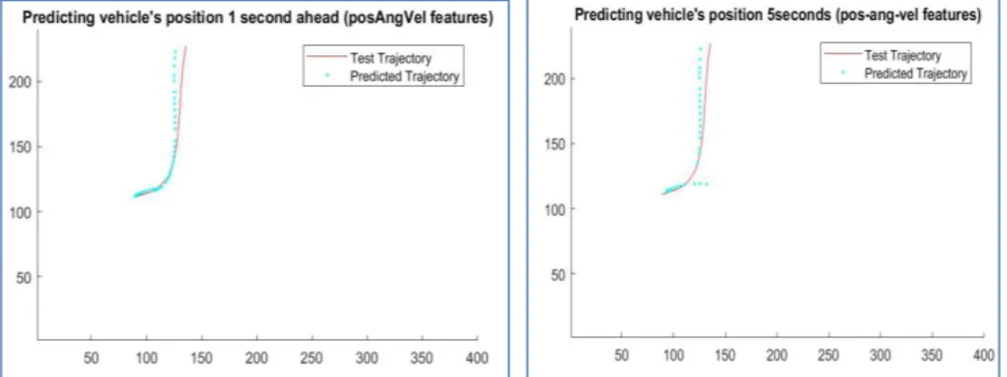
For instance, Figure 12 and Figure 13 show the algorithm for how to predict the behaviour by looking ahead after 1 second and 5 seconds respectively. The predicted position assigned by red x sign and a big circle illustrates where the future position of the current state of the observed Agent (marked by yellow square). The predicted future points drawn for the average trajectory (calculated by taking the average to all
Start points Endpoint
Endpoint Endpoint
Figure 10: Average reference trajectories (pedestrian).
Start point End point End point
category type that the agent belongs to. Where the size of the circle is increasing or decreasing depends on the given value for the sum of probability that calculates the particles’ weights that match the behaviour of the observed agent to any of the reference trajectories, that value is multiplied by 50 to make the circle big. The red thick line indicates the winning trajectory, which represents the most similar trajectory from the reference trajectories that match the features of the observed trajectory.
Predicted Position the Winning Trajectory Current Observed Agent’s position
Figure 12: Predicting the vehicle’s position after a second ahead.
Start point
Predicted Position the
Current Observed Agent’s position Winning
Trajectory
Figure 13:Predicting vehicle’s position after 5 seconds ahead.
Start point
Chapter 3
3 Rational of algorithm development
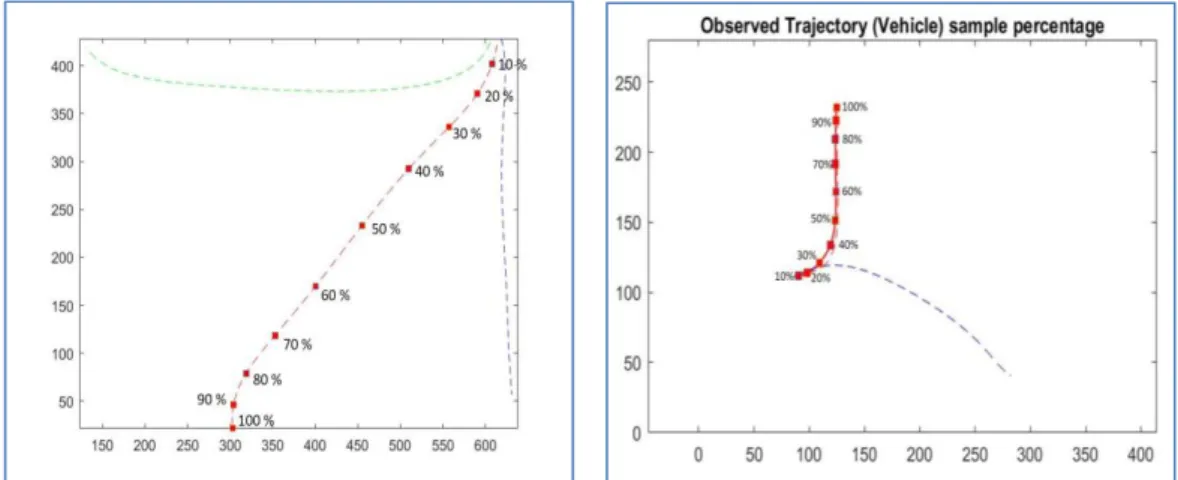
The starting point of the experimental work was to create an algorithm suitable for modelling the behaviour of other agents, the framework for modelling the behaviour. We started with a given a simulated set of reference trajectories and categorized them as (human, truck or vehicle). A number of experiments were done in the current work to check different options about how to select the number of reference trajectories and what kind of agents were suitable for this work. In this chapter, an example of an experimental procedure for developing the algorithm and its application in modelling the intention of other agents is given. In addition, we are going to illustrate some of the results after testing a moving agent (pedestrians and vehicles) and predicting its intention. The algorithm was tested using the dataset (28 Aug) from the Edinburgh Informatics Forum (ppedestrians) and the MIT trajectories (Vehicles) mentioned previously in section 2.1.1.
3.1 Implementation of the algorithm
A series of experiments were tested to explore the data set to find suitable agent trajectories for modelling. Then, after collecting these trajectories, we tried to find the best trajectories that are valid for classification. The way to classify these trajectories was explained previously in Chapter 2 in section 2.1.1. Many reported studies indicated that the angle is the best feature for estimating the agent’s intention either to turn or continue in its way. So, we choose the angle as an attribute to model the behaviour of other agents and categorize the intention to one of the defining categories. After that, we tried to test other features and compare it with the angle feature. For choosing the number of reference trajectories we started using only two trajectories from each category. Then, we gradually increased the number of reference trajectories and evaluated the accuracy.
Below, a presentation of the results for a PF algorithm that uses different map features for the same observed trajectory with the same 15 reference trajectories is given. The data referred to the Edinburgh Informatics Forum. The reference trajectories were used to model the behaviour, thus, we have 3 different behaviours and we use these behaviours to predict the intention where Agents (Pedestrians) intend to go. For the observed trajectory, we picked one from category 1 (assigned by red colour) and the reference trajectories included 5 trajectories from each category. As we have three categories which are Cat. 1 assigned as red colour containing 1-5 trajectories and Cat.2 assigned as blue colour containing 6-10 trajectories and Cat. 3 assigned as blue colour containing 11-15 trajectories used to train the algorithm, shown in Figure 14 and Figure 15. Finally, the algorithm was tested for five different numbers of reference trajectories from each category.
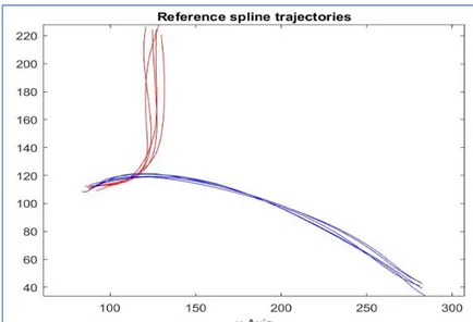
Also, we tested the algorithm with another data type extracted from MIT trajectories (Vehicles). We selected one trajectory as a test trajectory (Figure 16) and 10 trajectories as reference trajectories (Figure 17). We have only two categories, which are Cat. 1 assigned as the red colour containing the numbers of trajectories from 1-5 and Cat. 2 assigned as the blue colour containing the numbers of trajectories from 6-10 to train the algorithm.
End point
Start point
Figure 14:Test spline Trajectory “pedestrian”.
Start points Endpoints Endpoints Endpoint s
Figure 15:Reference spline trajectories used as training trajectories “pedestrians”.
In the next section, we show the practical procedure using these features whereby one presents the best feature to recognize the intention from an early stage. Predicting the goal for the test trajectory after the classification result referred to one of the different categories representing the subways that the agent may select.
Figure 16:Test spline Trajectory “Vehicle”.
Figure 17: Reference spline trajectories used as training trajectories “MIT dataset”.
3.1.1.1 Recognizing the Category of the agent
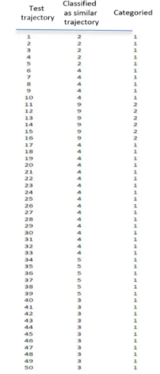
From each trajectory, we calculated the angles of agent trajectory and then tried to predict the estimated angle by matching with the angles of other trajectories, this was done by comparing the current angle of the observed agent with all the angles belonging to other current reference trajectories and so on. We tested a trajectory for pedestrians from category 1 (red) as in Figure 14 (pedestrian) and used the reference trajectories as in Figure 15 (pedestrians). The result is shown below in Table 1, Figure 18 and Figure 19.
.
Table 1: A classification result for observed trajectory from starting point to the goal (pedestrians)
Figure 18:Angles features for all the reference Trajectories.
References trajectories belongs to cat.3 have probabilities close to 0 because there are no similarities between them and the observed agent.
Figure 19: State Evolution for the belief of PF about the observed Agent for belonging to one of the three categories (Angle
Figure 18: shows map features (angles) for all reference trajectories in the three categories. Clearly, there is overlap between the angles from different categories at the start point and the end point of the trajectories. However, the algorithm was able to predict the similarity in the behaviour when the agent is moving ahead from the starting point toward the goal point. This is shown in Table 1, where, column (1) represents the number of the trajectory points (test trajectory) equal to 50 points. Each point refers to the state of agent and in this case, it contains the angles only. Column (2) contains the result after processing an agent’s angles and compares each angle with the current reference trajectories in each state of the 15 references. Obviously, from starting the algorithm categorizing the trajectory as similar to trajectory no. 9 which belongs to category 2 until 7th state. This is because of the overlaps between the angle’s
values in the starting points for the three categories shown previously in Figure 18. After that, the program able to estimate the correct category. Column (3) illustrates the category number that the reference number belongs to (either cat. 1, 2 or 3). Hence, the algorithm estimates the behaviour of observed agent and classifies the behaviour to a category according to the similarities between the Agent’s behaviour and the other reference trajectories.
Figure 19 denoted the probabilistic model of the state evolution, PF evaluated the probability distribution of state based on a set of observations from the reference trajectories. The value of probability describes how highly fitting the state to one from the reference trajectories that approximated by the measurement update at each moving step by a set of weighted particles. Given that the red colour (cat. 1) has the highest probability, it is subject to change according to the degree of symmetry between all reference trajectory features (angles). For example, in Figure 19 and Table 1 the state starts to be similar to trajectory no. 9 (cat. 2) then aligns to reference trajectory no.2, then reference trajectory no.5 and then no.3 and they all belong to the same category cat.1 which have the same properties. The result shows the tracking agent was classified correctly. We deduce, the algorithm is able to predict the correct classification as early from the 7th point forward the end trajectory points (goal).
Another classification of results using angles as features is presented below in Figure 20, Table 2 and Figure 21, using vehicles trajectories (MIT trajectories) implemented in the same algorithm. At the beginning, the algorithm is classified properly, the vehicle as reference trajectories belongs to cat1, which are reference trajectories 2 and 4 (illustrated in Table 2 column 2) but then classified wrongly as similar to ref. 9 which belongs to cat. 2. Thus it can be explained due to the overlap between the trajectories in the middle at intersection area as shown in Figure 20, where Figure 21 displays the state evolution of observed agent (vehicle) and how the estimation of test trajectory belonging to one of the ten (five for each category) reference trajectory.
Figure 20: Angles for all the reference Trajectories (vehicles). Table 2: A classification result using
angles features for observed trajectory (Vehicles) from starting
3.1.1.2 Predicting future position after second steps ahead
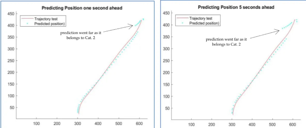
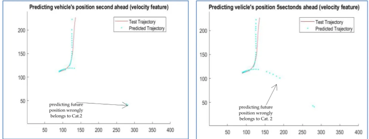
As mention previously in prediction section 2.1.4, that the algorithm is able to track the agent movement and predict where the agent will be after seconds ahead beyond classifying the behaviour according to defined reference trajectories. We considered the prediction as a long prediction after we deduced that the agent had followed a specific category. Thus, it allowed us to estimate the goal and where the agent will end up. Hence, we present the results of the prediction by tracking the agent’s angle behaviour.
Figure 22 shows the predicting of the future position of pedestrians, after 1 and 5-second steps ahead in order to estimate the agent’s intention. This was done by knowing the average speed of all the reference trajectories belonging to the selected category (selected by the PF method for the most similar category) and multiplying
Figure 21:State Evolution for observed Agent for belong to one from the two categories (Angle feature- vehicles).
prediction went far as it belongs to Cat. 2 prediction went far as it
belongs to Cat. 2
Figure 22: Short-term (1 sec) and Long-term (5 sec) Predicting position using angles features (pedestrian).
a long-term prediction. Therefore, the distance can be calculated, and the new position can be determined. The errors between the predicted point and the real point were calculated by Euclidean distance. The average of the errors was presented and compared. The trajectory in Edinburgh defined in pixels as image size 640 x 480. Therefore, each pixel horizontally and vertically corresponds to 24.7 mm on the ground. Thus, we converted the error from pixel to meter and the distance errors were presented in meters. In Figure 22 (predicting 1 second ahead) the average error was 0.2793 m, whereas it was around 0.3673 m after 5 seconds. We noticed that the error rate increased with long term prediction.
Figure 23 prediction position presented of vehicles after 1 and 5-second steps ahead using MIT trajectories., in which, the view of the camera at MIT was covering 1200 x 850 m and each pixel in trajectories approximately corresponded to 0.4 m/pixel. So, the distance error was approximated in meters. In Figure 23, (predicting 1 second ahead) the average error we got in meters was 2.2401 m. Whereas, the distance error in (predicting 5 seconds ahead) was around 4.5903 m.
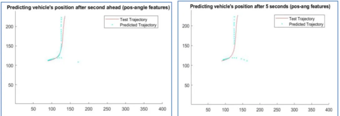
Using position as a feature:
In this section we present a classification of results using position as a feature. So, here we can observe the similarities through the appropriate behaviour (Position) for each state of agents. Similarly, for the procedure for angle feature, we used same test trajectory (cat.1) as in Figure 14 (pedestrian) and Figure 16 (Vehicle) and the same reference trajectories as in Figure 15 (pedestrian) and Figure 17 (Vehicle) that were mentioned previously for both Edinburgh and MIT datasets.
Hence Table 3, Figure 24 and Figure 25 illustrate the algorithm results using only a position parameter (x and y) to estimate the most similarity trajectory from reference trajectories (15 trajectories-pedestrians) to the observed trajectory (Pedestrian).
predicting future position wrongly belongs to Cat. 2
Figure 23:Predicting position Short (1 sec) and long-term (5sec) using angles features (vehicle).
predicting future position wrongly belongs to Cat. 2
algorithm to find similar position values from the early stage. Table 3 shows the detected reference trajectories and the predicted categories from the starting state to the end of the movement. It classifies the behaviour to Cat. 2 at the beginning and then correctly classifies to cat.1 (between 1-5 trajectories). But in states 21-24 it categorized wrongly to Cat. 3, similar to ref. no 15 according to some similarities in y- position. Figure 25 illustrates the state evolution probability for the belief most similar from all reference trajectories between 1-15 given by a higher probability.
Figure 26 shows the results of predicting position after a one second step ahead (sort-term) and a 5 seconds step ahead (long-(sort-term). For the short prediction, the average error we got was 0.5215 m. Whereas the average distance error in long-term prediction (predicting 5 seconds ahead) was around 0.5931 m.
Figure 24:Map position features for all the reference Trajectories (Pedestrians).
Table 3: A classification result using position features for observed trajectory (Pedestrian) from
Table 4, Figure 27 and Figure 28 show the results of vehicles from MIT trajectories used to model the behaviour of the agent (vehicle) using a position feature. Similarly, the algorithm was not able to classify the trajectories correctly at the early stage, but it improved afterward. The prediction after one second and 5 second steps ahead shown in Figure 29 and the average distance error in prediction for 1 sec is 2.4276 m and for long-term prediction is 4.7954 m.
Figure 25:State Evolution for observed Agent (Position feature- Pedestrians).
Figure 26: Short-term (1 sec) and Long-term (5 sec) Predicting position using position features (pedestrian) predicting future position wrongly belongs to Cat. 3 predicting future position wrongly belongs to Cat. 3