Department of Agricultural Research for Northern Sweden
Objective determination of marbling levels in
raw bovine meat
– using hyperspectral imaging
Objektiv bestämning av marmoreringsgrad i färskt nötkött – med
hjälp av hyperspektral bildanalys
Johanna Friman
Master´s thesis • 30 credits
Animal Science Umeå 2019
Objective determination of marbling levels in raw bovine meat –
using hyperspectral imaging
Objektiv bestämning av marmoreringsgrad i färskt nötkött – med hjälp av hyperspektral bildanalys
Johanna Friman
Supervisor: Mårten Hetta, Swedish University of Agricultural Sciences, Department of Agricultural Research for Northern Sweden
Assistant supervisor: Anders Karlsson, Swedish University of Agricultural Sciences, Department of Animal Environment and Health
Assistant supervisor: Julien Morel, Swedish University of Agricultural Sciences, Department of Agricultural Research for Northern Sweden
Assistant supervisor: Karin Wallin, Swedish University of Agricultural Sciences, Department of Animal Environment and Health
Examiner: Katarina Arvidsson Segerkvist, Swedish University of Agricultural Sciences, Department of Animal Environment and Health
Credits: Level: Course title: Course code:
Programme/education:
Course coordinating department: Place of publication: Year of publication: Cover picture: Online publication: Keywords: 30 credits
Second cycle, A2E
Självständigt arbete i husdjursvetenskap, A2E - Agronomprogrammet - husdjur
EX0872 Animal Science
Department of Animal Breeding and Genetics Umeå
2019
Johanna Friman
https://stud.epsilon.slu.se
meat quality, eating quality, tenderness, marbling, imaging technique, hyperspectral imaging, objective and subjective analysis
Swedish University of Agricultural Sciences
Faculty of Veterinary Medicine and Animal Science Department of Agricultural Research for Northern Sweden
Beef is a highly demanded food and plays an important role in the everyday diet for many people. The most common methods for measuring meat quality attributes are pH, colour, water-holding capacity, intramuscular fat, flavour and tenderness, are more or less performed by subjective methods and various types of chemical methods, which all are time consuming, invasive and de-structive. Furthermore, results from subjective measurements may be incon-sistent due to biased judgement. Different imaging-based techniques have re-cently been tested in order to rapidly and non-destructively measure and rank quality traits in beef cuts with consistent and reliable results. In this study imaging techniques (digital imaging and hyperspectral imaging) were used to objectively predict the average fat content and the distribution of fat on the surface of cuts of fresh beef samples.
One part of this project digital (RGB) images from 61 beef samples were provided (from an earlier completed scientific study and analysed. Separately from the imaging analysis, it was evaluated how different traits such as age and breed affected the level of marbling. For each image there was back-ground information with traits (carcass characteristics and slaughter data), that was analysed using a principal component analysis (PCA). Both breed and age affected the marbling grade, but the marbling was not affected by carcass characteristics.
In the other part of the project, a set of 120 commercially provided beef sam-ples were analysed using a hyperspectral camera. In order to acquire the hy-perspectral images, a hyhy-perspectral imaging system with a spectral range of 900-2500 nm was used.
Images from both datasets were analysed to obtain objectively measured fat content of all image samples. The predicted fat contents were then compared with marbling grades, evaluated by an experienced grader.
The results from the image analysis indicate that both imaging techniques can be used to predict the amount and distribution of fat in beef samples, however in terms of overall accuracy, the hyperspectral imaging system was more pre-cise. The comparison between measured fat content and marbling grading in-dicate that there is a correlation between higher fat content and higher
bling grade. However, there is a low correlation between the visually meas-ured (marbling grading) and objectively measmeas-ured (RGB and HS imaging) fat content, for both the RGB dataset and the hyperspectral dataset.
Keywords: meat quality, eating quality, tenderness, marbling, imaging tech-nique, hyperspectral imaging, objective and subjective analysis
Nötkött är en mycket efterfrågad råvara som spelar en viktig roll i mathåll-ningen för många människor. De nuvarande metoderna för mätning av kvali-tetsattribut som pH, vattenhållande kapacitet, intramuskulärt fett, smak och mörhet är manuell inspektion och olika typer av kemiska analyser. Metoderna är tidskrävande och destruktiva, dessutom kan mänskliga klassificeringar vara inkonsekventa. Olika typer av bildanalyser har nyligen studerats för att kunna snabbt och icke-destruktivt mäta och rangordna kvalitetsegenskaper i styckdetaljer med konsekventa och tillförlitliga resultat. I denna studie an-vändes bildanalys för att objektivt bestämma det genomsnittliga fettinnehållet och fördelningen av fett på ytsnitt av färska ryggbiffar.
RGB-bilder tillhandahölls (från en tidigare avslutad vetenskaplig studie) och analyserades. Separat från bildanalysen utvärderades hur olika faktorer på-verkar marmoreringsgraden. Bakgrunds information (produktion, slakt och slaktkropp), som korrelerade med RGB-bilderna, analyserades med hjälp av en principalkomponent analys (PCA). Både ras och ålder påverkade marmo-reringsgraden, men marmoreringen skilde sig mellan djur av samma ras och ålder.
Separat från RGB-data användes en uppsättning av 120 biffprover för att ge hyperspektrala bilder. För att förvärva hyperspektralbilderna användes ett hy-perspektralt bildsystem med en bandbredd på 900-2500 nm.
Båda dataseten analyserades i bildhanteringsprogramvara för att erhålla ob-jektivt analyserade fettinnehåll i alla bilder. Det obob-jektivt bestämda fettinne-hållet jämfördes sedan med den grad av marmorering som bestämts genom visuell inspektion (subjektivt).
Resultaten från bildanalysen indikerar att både RGB bilder och hyper-spektrala bilder kan användas för att objektivt bestämma mängden och för-delningen av fett i nötkött, men vad gäller noggrannhet var det hyperspektrala bildsystemet bättre. Det objektivt bestämda fettinnehållet korrelerades emel-lertid inte med den subjektiva graderingen, vilket indikerar att det finns skill-nader i skattningar för både RGB-datasetet och den hyperspektrala datasetet. Nyckelord: köttkvalitet, ätkvalitet, mörhet, marmorering, bildanalys, hyper-spektral bildanalys, objektiv och subjektiv analys
Intresset för kött av hög kvalitet och välutvecklad marmorering (intramusku-lärt fett) har ökat bland konsumenter och branschintressenter. Marmorering anses idag vara en tydlig markör för kött av premiumkvalitet. Det finns en efterfrågan på en effektiv och noggrann metod för att kunna mäta marmore-ringen i en slaktkropp med hög precision och med konsekvent resultat. Bedömningen av
marmorerings-grad förslaktkroppar utförs idag av utbildade inspektörer på landets slakterier. Metoden för klassifice-ring är dock tidskrävande och trots ett vältränat öga kan en visuell be-dömning innebära inkonsekventa bedömningar av slaktkropparna. Att objektivt kunna mäta marmo-rering, skulle kunna bidra med högre noggrannhet i bedömningen och mindre variation mellan t.ex. slakterier och bedömmare. Flerta-let studier har gjorts för att utvär-dera om bildanalys kan användas för att gradera slaktkroppar och bedöma kvalitetsegenskaper såsom mörhet, smaklighet och saf-tighet.
En metod som visat hög potential är hyperspektral bildanalys (HSI). I motsats till det mänskliga ögat som ser synligt ljus (rött, grönt, blått), fördelas spektral bildanalys över flera våglängder utanför det
synliga spektrat. Detta ger möjlig-het att se det som inte går att se med blotta ögat.
I denna studie användes HSI för att objektivt analysera andel fett samt distributionen av fett i rygg-biff. Samma ryggbiffar bedömdes visuellt av en tränad bedömare och graderades efter mängden marmo-rering. Den visuella bedömningen jämfördes sedan med HSI resulta-tet. I studien användes och analy-serades även fettinnehåll i kött från ett annat dataset fotade med vanlig RGB-kamera. Resultaten visar att HSI generellt hade bättre klassificering av fettinnehåll än RGB-bilder.
Studien påvisade möjligheter hos bildanalys i allmänhet, men HSI i synnerhet att objektivt kunna be-döma andel fett i en köttbit. Det är av intresse att fortsätta utveckla hyperspektral kamerateknik för att snabbt och med hög precision kunna bedöma marmoreringsgra-den i olika styckdetaljer.
Bildanalys för en mer konsekvent och noggrann
bedömning av marmoreringsgrad
1 Introduction 9
1.1 Objective 9
1.2 Background 9
1.3 Quality challenges in the meat industry 10
1.3.1 Carcass grading in Europe 10
1.3.2 Beef quality 12
1.3.3 Eating quality 13
1.3.4 Traits affecting marbling 15
1.3.5 Restrictions 16
1.4 Imaging techniques 16
1.4.1 RGB imaging 16
1.4.2 Hyperspectral imaging 17
1.4.3 Differences between RGB and HS imaging 17
2 Materials and methods 22
2.1 Data acquisition 22
2.1.1 SKARA dataset 22
2.1.2 Hyperspectral dataset 23
2.2 Image pre-processing 25
2.3 Mathematical models used for classification and quantification 26 2.4 Principal component analysis of the SKARA dataset 27
2.5 Image analysis 28
2.5.1 Supervised classification of pixels to train reference data 28
2.5.2 Effect of plastic package 29
2.5.3 Analysis of fat distribution of both sides of the cut 30
3 Results 31
3.1 Correlation of the SKARA dataset variables 31
3.2 Training of pixel data for modelling classification and quantification 34
3.2.1 RGB images 34
3.2.2 Hyperspectral dataset 35
3.2.3 Effect of plastic package 37
38
3.2.4 Analysis of fat distribution of both sides of the cut 39 3.3 Comparison of objective fat analysis and subjective marbling grading 42
3.3.1 Comparison of the accuracy between RGB image and HS image
based analysis 43
4 Discussion 44
4.1 Intercorrelation of the SKARA dataset variables 44 4.2 Classification and quantification of the meat components 45
4.2.1 SKARA dataset 45
4.2.2 Hyperspectral dataset 46
4.2.3 Effect of plastic package 47
4.2.4 Analysis of fat distribution of both sides of the cut 48 4.3 Comparison of the accuracy of the models built on RGB and HS images 49
5 Conclusions 51
References 53
9
1 Introduction
1.1 Objective
The overall objective of this study was to evaluate if imaging systems could be used to estimate the average fat content and the distribution of fat on the surface cuts of fresh beef samples.
The specific objectives were to:
1) Connect background information of the animals and marbling grade to eval-uate the connection between different animal traits and marbling.
2) Compute the distribution of intramuscular fat in beef samples, using an im-aging system.
3) Evaluate two imaging systems on their potential to estimate the fat distribu-tion in beef: RGB images and hyperspectral images.
4) Compare the fat distribution results from the objective analysis with mar-bling grades from a subjective analyse to see if an imaging system can be used to estimate marbling in beef.
1.2 Background
In the modern beef industry, cattle origin from farms, where a range of production systems are used, e.g. from intensively production based on grain to extensive pro-duction based on grazing. The systems also fits better for different types of breeds, thus animals with different carcass characteristics are used such as dairy breeds, light beef breads and Heavy beef breads. Also differences between the three sex, intact females, intact bulls, castrated bulls do exist. All these production factors af-fect the quality of the meat provided after slaughter, and with the many different production systems, the industry is struggling to keep a consistent quality level (Naganathan et al. 2008). Since beef is a highly demanded food component and also commonly an important part in the everyday diets for many people, it is of high interest to be able to guarantee the quality of meat and meat products (Aredo, Velásquez, and Siche 2017).
From a consumer’s point of view, beef quality can be defined by two main factors related to either (i) eating experience and (ii) hygienic quality. Consumers expect a product to be hygienically safe and free from pathogenic microbes. Being able to supply the costumer with safe products is considered to be one of the most important objectives in the industry (ElMasry G and Sun D.-W 2010; Kamruzzaman and Sun
10
2016). However, quality attributes in beef refer mostly to the eating experience. The eating experience is controlled by several traits as e.g. pH, water-holding capacity, fat- and protein- content and tenderness. Among all those attributes, tenderness is the most important factor influencing the eating quality. Consumers are willing to pay more for beef, if they are guaranteed a tender meat and refer to tenderness as the primary factor in eating satisfaction (Aredo, Velásquez, and Siche 2017; ElMasry G and Sun D.-W 2010; Kamruzzaman and Sun 2016).
As the demands of products with high eating quality increases, it would be of interest to start evaluating the factors that correlated with attributes such as tender-ness, flavour and juiciness. The traditional method for measuring the tenderness is by measuring the mechanical properties of the beef, Warner–Bratzler shear force (WBSF) or slice shear force (SSF). Such methods are time-consuming and destruc-tive, by means that they are performed on cooked meat and the samples are cut. Other methods rely on human inspectors, such as sensory evaluation by trained ex-perts. This method is both time consuming and limited by the subjectivity of each operator, which may give inconsistent and biased results (ElMasry G and Sun D.-W 2010; Park et al. 2001). It is therefore desirable to find a cost-effective and fast way to evaluate factors that affect the eating quality to meet the consumers demand for high quality meat (Park et al. 2001; Jackman, Sun, and Allen 2011).
1.3 Quality challenges in the meat industry
1.3.1 Carcass grading in EuropeIn most European abattoirs, Swedish included, a system called EUROP is used to manually evaluate and grade the carcasses based on their conformation and fatness. The system is designed to ensure a fair and equal payment to the producer among all slaughter facilities. Furthermore the conformation scoring can be used (i) as a quality marker, (ii) to give feedback to the producer and (iii) to sort carcasses for further processing and selected markets (Einarsson 2011). The system is not built on evaluating the eating quality of single cuts, but mainly focuses on the primary yield factors of the carcass such as fat content and muscle conformation (Einarsson 2011; Konarska et al. 2017). The value of a carcass is highly dependent on the sale-able meat yield, which will be determined by the total fat percentage in the carcass and the amount of lean meat (Craigie et al. 2012).
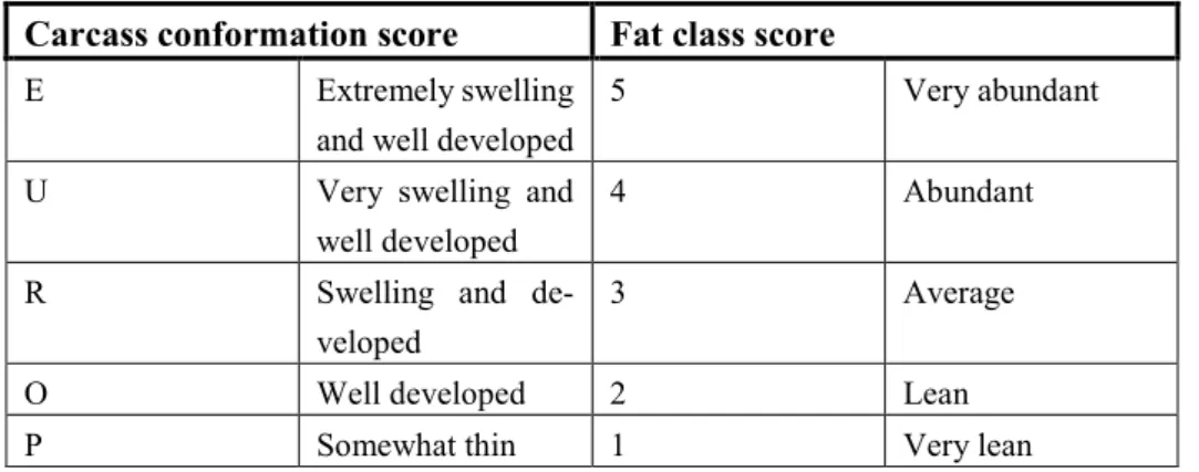
11 The carcass is scored in fat class and conformation class, conformation is scored from E-P, and fat class is scored from 1-5. The scores are illustrated in Table 1. Each score can additionally be graded with +/-, hence the EUROP classification system has 15 classes.
Table 1 Classification of carcasses according to EUROP (Jordbruksverket 2002)
Carcass conformation score Fat class score
E Extremely swelling and well developed
5 Very abundant U Very swelling and
well developed
4 Abundant R Swelling and
de-veloped
3 Average O Well developed 2 Lean P Somewhat thin 1 Very lean
The lowest grading is thus equal to P- for conformation and 1- for fat class. The conformation class describes the swelling and amount of flesh on the carcass whereas fat class indicate the amount of subcutaneous fat on the outside of the car-cass (Einarsson 2011; Johansen et al. 2006). In general, carcar-casses from specialized beef breeds gain higher conformation classes due to higher weights and higher dressing percentage. They also deposit less subcutaneous fat and show lower fat classes when compared to dairy cattle. The beef breeds ability to transform nutrients mainly into protein and to gain muscle instead of deposit fat contribute to their higher carcass conformations scores (Albertí et al. 2008; Clarke et al. 2009). All grading is performed based on photographic standards and the graders are highly educated and trained. The graders are regular inspected by the Swedish Board of Agriculture to confirm the standardisation among all graders. However, even if eval-uators are well trained, the subjectivity within visual assessment may results in in-consistency within the classification of carcass conformation due to human error (Craigie et al. 2012; Johansen et al. 2006). When the classification accuracy of eval-uators in Norway was tested, systematic differences were found between classifiers. However the differences were within the limits for validation stated by the EU com-mission. It was concluded that the evaluators in general over-classified confor-mation and under-classified fat class (Johansen et al. 2006).
Several studies have been conducted in order to estimate the accuracy of classifica-tion in the EUROP system. Comparison has been made between the EUROP system
12
and image analysis, to evaluate the accuracy of both objective and subjective sys-tems (Craigie et al. 2012; Einarsson 2011; Johansen et al. 2006). In the study of Johansen et al. (2006), the results indicated systematic differences between operators and European standards, however they were within the limitations stated by the EU comission. Craigie et al. 2012 and Einarsson 2011 concluded that current, subjetive grading has shortcomings due to inconsistency between operators. They both compared the visual grading with objective systems and proved that imaging assessment could be used with good results, when they were compared to the results based on the EUROP grading system.
1.3.2 Beef quality
Beef quality is defined as a combination of traits covering both composition of the beef (e.g. lean to fat ratio, meat percentage, intramuscular fat), sensory traits and functional traits (visual appearance and eating quality).
Functional traits include for instance water-holding capacity (WHC) and pH, whilst composition traits cover e.g. lean to fat ratio, meat percentage, nutritional value, fat content and composition, and marbling. Sensory traits are those factors that affect the eating quality or palatability such as flavour, juiciness and tenderness (Andersen et al. 2005; ElMasry G and Sun D.-W 2010).
Over the past decade, a higher knowledge about animal welfare and environmental impact from animal production have led to new standards regarding quality meat. Consequently, the definition of high quality now includes the production condition such as management, feeding and pre-slaughter handling (Andersen et al. 2005). One of the biggest issue in predicting quality of beef is that several factors will affect the traits listed above, both ante-mortem and post-mortem. Preslaughter stress and post-mortem factors such as changes in pH, cooling and aging, handling during packing and transport of the meat all influence the final quality attributes of the product.
Ante-mortem factors that highly influence the characteristics of the meat are breed, sex, age and feeding. Also the management during lifetime, transport to slaughter and slaughtering conditions will affect the carcass characteristics (Y. Liu et al. 2003; Miller 2002).
How familiar the animal is to human contact and if it is comfortable being trans-ported and handled by man is a crucial factor for the physical properties of the meat. An animal that is not used to being transported or handled may become very stressed
13 during transport to slaughter and/or at the slaughterhouse. The acute stress will af-fect the quality of the raw meat in a negative way due to a rapid decrease in pH (Grandin 1980).
1.3.3 Eating quality
Consumers consider tenderness to be the most important quality factor when deter-mine the eating experience (Park et al. 2001). In a consumer panel test (Lucherk et al. 2016) 252 panellists ranked flavour and tenderness as top most important palat-ability traits when eating beef. The purchasing habits of 120 panellists participating in a sensory test showed that more than 50 percent of the participants ranked ten-derness as the most important palatability trait, followed by flavour and juiciness (Corbin et al. 2015).
Tenderness is commonly measured by either sensory tests, performed by consumers and/or trained test panels or by instrumental technique. Usually the tenderness is measured using Warner-Bratzler shear force (WBSF) or slice shear force (SSF). The objective with both methods is to measure the force needed to cut through the centre of cooked steak samples (ElMasry G and Sun D.-W 2010). Older animals have less tender meat than young animals. This is due to collagen crosslinks, which changes the mechanical properties of the intra muscular connective tissue and contributes to the toughening of meat (Nishimura 2010). It is proven that marbling levels and the tenderness of meat is positively correlated (Xiong et al. 2014). As marbling is de-posited into the muscle between the collagen linkage, it weakens the connective tissue resulting in tenderisation of the meat (Miller 2002; Nishimura 2010).
Intra muscular fat (IMF) has an important role in different eating quality traits. The visible amount of IMF in the muscle is referred to as marbling. Marbling will appear in the muscle as small, thin streaks (like a marble pattern). The amount of streaks
Figure 1 Degree of marbling will be determined on the amount of thin fat streaks within the muscle, and how well they are spread over the surface. The right beef cut is graded higher due to more fat streaks and how well they are distributed. High amount of fat streaks but poor distribution will be assigned a lower marbling grade.
14
and how well they are spread over the surface of the cut will determine the degree of marbling (Figure 1).
Marbling is one of the most important features that influences the sensory accepta-bility of meat and meat products. It affects all the attributes that are demanded by consumers such as flavour, juiciness and tenderness (Miller 2002).
It is also shown that intensity of flavour increases with marbling levels (Miller 2002). Uniformly and fine distribution (evenly spread over the surface of the cut) of
fat streaks is to prefer. A steak with a high amount of finely distributed fat streaks will be considered to be of superior quality (Velásquez et al. 2017; Xiong et al. 2014).
In a study performed by (Lucherk et al. 2016), the palatability of beef steaks with varying marbling level and cooked to three different degrees of doneness were eval-uated. The results indicated that the SSF value of beefsteaks significantly decreased when marbling level increased. The effect of doneness was also affected by mar-bling. The most marbled samples managed to sustain its juiciness even when it was cooked to well-done (highest degree of doneness) and it also remained most tender compared to other marbling levels.
The relation of tenderness and marbling level was concluded in (Corbin et al. 2015). According to this study, both juiciness and tenderness were correlated with fat con-tent and increased with increased fat percentage. The correlations between tender-ness, juiciness and flavour is strong and fat percentage plays a big role in all three factors.
Since tenderness is considered to be the mostly important factor for eating quality, and since it is highly correlated with degree of marbling, it is important that mar-bling is accurately predicted (Park et al. 2001; Konarska et al. 2017). The USDA quality grading system is a classification system that aims to grade carcasses based on both conformation and marbling. The scale consist of nine different levels of grading. In Sweden, the grading of marbling is based on the American USDA scale, but its nine levels is edited to fit Swedish cattle. Hence it only consists of five classes ranging from level 1-5 (Table 2). The grading is based on reference cards which represent the standard for marbling (Stenberg 2013).
Another system for grading carcasses is the Meat Standard Australia (MSA), founded in Australia. The system includes the carcass conformation scoring like EUROP system. However, carcass grading in Australia also include several factors that will affect the eating quality. Those factors include breed, age, sex marbling, growth of the animal, carcass attributes and processing methods.
15 Like the EUROP system, the grading is performed by trained assessors, however it considers more traits in order to guarantee high quality meat and tenderness of beef cuts for costumers (Aus-Meat 2018).
Table 2 Swedish standard for marbling levels (Stenberg 2013).
Marbling level Definition USDA – equivalent
1 No marbling -
2 Incipient marbling Small
3 Marbled Modest
4 Well marbled Moderate
5 Very marbled Slightly abundant
Today no rapid, consistent and non-destructive method exist to predict marbling levels. Visual evaluation is time-consuming and rely on subjective inspections, which may be inconsistent. Instrumental methods are convenient and effective in measuring tenderness. However they are time-consuming, destructive and often re-quires long-time sample preparation (Xiong et al. 2014).
For marbling grading to become time-effective and accurate, it is needed to develop objective and automatic systems. Since the demand for high quality meat increases, many efforts have been made to develop non-destructive techniques for assessing marbling levels. Different types of imaging systems used for detecting traits such as tenderness and marbling have been developed and tested. The results indicate that imaging systems are powerful tools for predicting quality attributes in meat (Park et al. 2001; Velásquez et al. 2017; Xiong et al. 2014).
1.3.4 Traits affecting marbling
Several animal traits will affect the marbling development in the beef. Older animals tend to be more marbled than younger, due to intramuscular fat being the last fat to deposit (Albrecht et al. 2006; Venkata et al. 2015).
Sex also influence marbling development. Heifers, in general receives higher mar-bling grades than steers. This may be due to heifers capability to deposit fat into the muscle (Venkata et al. 2015). In an article (Harper and Pethick 2004) it was con-cluded that heifers tend to be more marbled than steers and bulls, steers being more marbled than bulls. However, steers had slightly higher marbling than heifers when IMF % was expressed in relation to total fatness. Beef from heifers generally appear
16
to be more juicy and tender, which is most likely to be related to their higher IMF content (Venkata et al. 2015; Węglarz 2010).
When comparing breed related changes in marbling, it is shown that Holstein ani-mals tend to have high number of marbling flecks. It is finer structured than other breeds and the flecks is intensively incorporated into the muscle at 6 months of age, comparable with 12 months for Angus (Albrecht et al. 2006). The percentage of subcutaneous fat where higher in Holstein bulls than Charolais bulls. The beef bull also showed overall lower amount of inner fat depots. The Holstein bulls had lower dressing percentage and lower carcass conformation but graded higher in marbling (Pfuhl et al. 2007).
1.3.5 Restrictions
Beef quality is a wide definition, influenced by both ante-mortem factors such as breed and genetics, dietary influences and management. The quality is also affected by post-mortem factors both directly at slaughter and after the slaughtering process, during production. All factors that affect the meat quality will have impact on the eating experience in several ways, and is an attribute that is effected by many dif-ferent factors. However, other important factors (other than marbling) linked to meat and eating quality (such as collagen, colour, pH and water holding capacity) will not be considered. Marbling as a quality factor and how it can be measured will be the main focus area in this report. Effects of breed, sex and age in marbling devel-opment will be taken in to account, but environmental and management factors will be excluded from the study.
1.4 Imaging techniques
1.4.1 RGB imagingAn ordinary digital camera takes photos that covers the spectral range of human vision and include wavelengths of approx. 400-700 nm. An RGB image consist of three spectral bands, red (R), green (G) and blue (B). The colours that we see are combinations of these three colours. The low number of spectral bands limits the RGB imaging in such way that it can have a high spatial resolution (many pixels per area), but poor spectral resolution and thereby less chemical information (Konda Naganathan et al. 2008).
17 1.4.2 Hyperspectral imaging
The characteristic for hyperspectral imaging (HSI) are the number of spectral bands in the image. Depending on the system, the number of spectral bands can reach to about 300 bands. Although the spectral bands are narrow, ranging from 1-10 nm, they provide lots of spectral information. The most widely used hyperspectral im-aging systems covers the visible wavelengths (380-800 nm) and the infrared range (400-1000 nm) (ElMasry and Sun 2010). A HS imaging system can be used to ac-quire images of both high spatial and spectral resolution, since it consist of both the digital camera (spatial information) and a spectrograph (spectral information) (Konda Naganathan et al. 2008).
With its ability to provide images with high spatial and spectral information, hyper-spectral imaging has become an interesting technique for non-destructive analysis of beef and other food products. Several research efforts have been made to develop an imaging system for rapid analysis of different attributes such as moisture, pH and fat content. For instance one study evaluated an imaging system for on-line fat meas-urement of beef trimmings. In slaughter facilities, beef trimmings are a residue from the deboning. The trimmings are valued by its fat content and often sold in batches with varied fat content and different size. The study aimed to calibrate an imaging system for measuring fat content of both single beef trimmings and for total amount of fat content in different sized batches. The imaging system accurately estimated the fat content in both single trimmings and for the different sized batches (Wold et al. 2011).
1.4.3 Differences between RGB and HS imaging
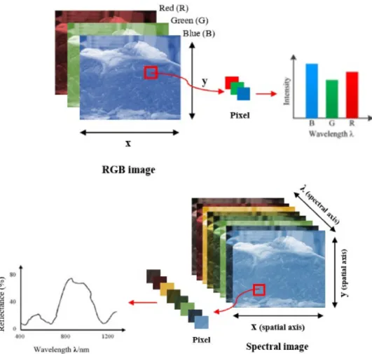
The main difference between a RGB image and a hyperspectral image is the richer spectral information provided by hyperspectral imaging. Figure 2 illustrates the dif-ferences between RGB spectral bands and the spectral bands in hyperspectral ages. The RGB images have a few very wide bands, whereas the hyperspectral im-age consists of hundreds of almost continuous, narrow bands. The amount of narrow bands enables an almost continuous reflectance spectrum for each pixel in the hy-perspectral image. That spectral information can then be used to classify and char-acterize objects (Gowen et al. 2007). Figure 3 illustrates the spectral curve for a fat pixel, obtained from an hyperspectral imaging compared to an RGB image..
18
Figure 2 Illustration of the spectral bands and wavelengths of RGB and Hyperspectral images. The RGB range consist of three wide bands (red, green, blue) whereas the hyperspectral image consist of hundreds of narrow bands. The amount of narrow bands allows an almost continuous reflectance spectrum for each pixel in the hyperspectral image.
Figure 3 Spectral differences between a fat pixel from an RGB image (above) and a hyperspectral image (lower). For the upper, the spectral information in the pixel is limited due to less spectral in-formation in the RGB image. The lower figure shows the spectral inin-formation generated by hyper-spectral imaging. The pixel gets a continuous spectrum, which can be used to identify objects based on its composition. The spectrum characteristics will act like a “fingerprint”.
19 In HS imaging, each pixel contains spectral information. This spectral information is added as a third dimension to the spatially-dependent two-dimensions image ac-quired by the system. The tree-dimensional image with two spatial and one spectral dimensions, is referred to as a hypercube (Gowen et al. 2007; L. Liu and Ngadi 2014). The whole spectral image can be referred as a hypercube, or each pixel can be extracted from the image as a pixel hypercube. The most simple hypercube is the RGB image where each pixel has red, blue and green colour, compared to a HS data cubes which can contain reflectance of up to hundreds of spectral bands (Figure 4) (Lu and Fei 2014; Vasefi, MacKinnon, and Farkas 2016).
Figure 5 illustrates in detail the extraction of a single pixel from the spectral image. The pixel from a RGB image will generate an intensity curve showing how much of the colour red, green or blue that is represented in the pixel. The pixel hypercube generated in the HS image generates a spectral curve, which provides a spectral signature for that specific pixel and does so for each pixel in the image. When ana-lysing spectral images, it is done on pixel level, using the spectral information in each single pixel and comparing the spectral signature to discriminate between dif-ferent constituents (Lu and Fei 2014).
Figure 4 Differences of spectral bands between RGB (left) and a hyperspectral image (right). The left RGB show the 3 spectral bands, red, green and blue. The hyperspectral image shows the 3-D “hypercube” consisting of the two spatial and one spectral dimension. It illustrates the high dimen-sion of information that can be generated from a hyperspectral image, when all spectral bands are merged into one hypercube.
20
Imaging systems based on RGB are often used in food quality systems, as they pro-vide a cheap and user-friendly imaging tool. However, they have limited abilities to detect surface features that are sensitive to wavebands other than RGB colours. This limitation is overcome with the richer spectral information of HSI-systems, making it possible to determine both physical and chemical properties in an object (Gowen et al. 2007; Huang, Liu, and Ngadi 2017)
Hyperspectral imaging systems and RGB based techniques have been compared in several studies. Systems based on RGB are user friendly and cheap imaging tech-niques widely used in food quality controls (Taghizadeh, Gowen, and O’Donnell
Figure 5 The RGB image (upper) consist of three spectral bands (red, green and blue). Each pixel will contain different amount (intensity) of each colour which will result in the visible colour compo-sition of the pixel. For the spectral image (lower), the extracted pixel gets an almost continuous spectrum. This generates a spectral signature for that specific pixel. With its spatial information it is possible to locate the pixel in the image and the source of the spectrum. Each pixel in the image has a spectral signature, enabling identification of constituents in different target objects.
21 2011). However, hyperspectral imaging system have shown higher levels of dis-crimination when used for sorting objects of different quality attributes (Al-Mallahi, Kataoka, and Okamoto 2008; Garrido-Novell et al. 2012).
22
2 Materials and methods
This report includes analysis and results from two independent datasets. The two datasets are treated separately as two separate studies.
The first dataset (hereinafter referred to as the SKARA dataset) included 61 RGB images of sirloins (Latissimus dorsi). These data were provided from a finished sci-entific project at the research facility SLU Götala Beef and Lamb Research, Swedish University of Agricultural Sciences, Skara.
The second dataset consisted of 120 samples of sirloins (Beef cuts), provided from a slaughter facility in Luleå (Nyhléns Hugosons, Luleå). This dataset will be referred to as the hyperspectral dataset (HS dataset), since the beef samples were used to provide hyperspectral images.
2.1 Data acquisition
2.1.1 SKARA datasetThis dataset consists of 61 RGB images, one example is shown in Photo 1. Each of the images have associated information of e.g. breed, age at slaughter and marbling
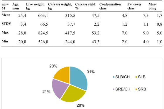
grade. This information will be referred to as the external spreadsheet since it con-tains variables that will be analysed, but not originated from the image analysis. The descriptive statistics of the data in the spreadsheet is illustrated in Table 3. This data were acquired from a scientific project (“Uppfödning av mjölk/köt-traskorsningsstutar”) on comparing pure dairy breed steers with crossbred steers. The aim of the project was to test if crossing dairy cows with a Charolais bull would increase growth, feed conversion, muscle coverage and fat coverage of the calves.
Photo 1 Red Green Blue ( RGB) image of sample 3 from the SKARA dataset
23 The images show a surface cut from a sirloin and include a code that links the image with information from the live animal and also slaughter data. The distribution of breeds in the dataset are illustrated in Figure 6. The marbling evaluation was man-ually conducted by an experienced grader. The subjective evaluation was used to compare the results from the image based classification models. This gave the op-portunity to compare objective and subjective results.
Table 3 Descriptive statistics of the traits in the external information sheet for the SKARA dataset. Number of observations for each trait = 61.
nn =
61 Age, mon Live weight, kg Carcass weight, kg Carcass yield, % Conformation class Fat cover class Mar-bling Mean 24,4 663,1 315,5 47,5 4,8 7,3 1,7
STDV 3,4 66,5 37,7 2,2 1,2 1,1 0,8
Max 28,0 824,5 417,5 53,2 7,0 9,0 5,0
Min 20,0 526,0 244,0 43,3 2,0 4,0 1,0
2.1.2 Hyperspectral dataset
For the hyperspectral imaging study, sirloin steaks (n=120) were provided from a local packaging plant (Nyhléns Hugosons, Luleå). The samples were single packed in plastic and vacuumed at the packaging plant. All samples were cut and packed to fit for commercial use and chosen by employees at the plant to provide a wide var-iation in total fat distribution among the samples.
Samples were kept in a cold room at a maximum temperature of approximately 4oC for 24 hours before the day of measurement. As differences in temperature can affect
31% 28% 21% 20% SLB/CH SLB SRB/CH SRB
Figure 6 Distribution of breeds in SKARA dataset. SLB = Swedish Holstein, SRB = Swedish Red, SLB/CH and SRB/CH = the crossbreeding with Charolais bull.
24
the comparability of the images, the samples were kept in a cool box with ice on the day of measurement.
To be able to analyse the effect of plastic package and also compare the fat content and distribution from the surface area on both sides of the sample, 20 samples were randomly chosen and scanned both with and without plastic. The sample was then turned and scanned again (without plastic) from the opposite side. These samples were thus scanned thrice, first with the plastic still intact, then with the beef taken out of the plastic with the same side facing up and finally scanned on the other side. The sirloin steaks were imaged using a ViaSpec Hyperspectral imaging system, completed with a motor driven transmission stage, a focus grid and a white reference (Middleton Spectral Vision, Middleton). The system is mounted with a push broom Specim short-wave infrared (SWIR) camera, using a 15 mm f/2.1 lens (SWIR spec-tral camera, SPECIM, Finland). The acquired images consisted of 288 specspec-tral bands, ranging from 935-2457 nm with a spectral resolution of 12 nm and a spatial resolution of 0.42 mm. The system was controlled by the Breeze software (Breeze, Prediktera AB, Umeå). Halogen light sources (bulbs) were used to illuminate the samples and were angled approximately 30o (to the horizontal plane) to focus the light beam to the whole surface area, without shadowing. The set-up is shown in Photo 2.
For each sample, the camera took a dark and white reference. Those references will eventually be used to compute reflectance (Schaepman-Strub et al. 2006), making all the images comparable in terms of spectral response.
25
2.2 Image pre-processing
In order to analyse the images, the background (i.e. everything that is not protein or fat) had to be removed from the image. This was done using a principal component analysis (PCA) implemented in the Breeze software (Prediktera, Umeå, Sweden) for the hyperspectral images. A PCA is a useful tool to visualize variation and pat-terns among variables in a large dataset. It reduces and transforms the original data into a set of principal components (PC) that explains the most of the variation in the data, where the first PC (PC1) holds the most variation, PC2 second-most etc. For the RGB images, the background was removed manually due to the more com-plex background and the poorer spectral information using Photoshop CS6 (Adobe, San Jose, California).
In order to make the RGB images comparable, the spatial resolution was homoge-nised for all images, using the image size application in Photoshop. The RGB im-ages was then loaded into Breeze.
Photo 2 The hyperspectral imaging system used for scanning beef samples (left). Prepared beef sam-ple (right)
26
2.3 Mathematical models used for classification and
quantification
For building the quantification model a partial least square regression (PLS-R) model was used. The aim was to quantify the percentage of fat and its distribution in the surface of the beef samples. The PLS-R specifies the linear relationship be-tween the response variable Y (in this case % of constituent, e.g. fat/muscle tissue) and the predictor variables X (in this case spectral value). It finds components in such a way that the score values have maximum covariance (Abdi 2007). In this study, the PLS-R was used to quantify the amount of fat and muscle tissue (referred to as protein in this report) in surface of the beef samples.
For the classification of pixels into classes of either fat, protein, background or plas-tic, a partial least squares-discriminant analysis (PLS-DA) was used. The PLS-DA maximises the variance in the data based on the classes of the dataset. The method aims to find a separator between two or more variables and group them, creating a straight line that divides the groups into different regions (Brereton and Lloyd 2014).
The PLS-DA is derived from PLS-R and unlike PLS-R, PLS-DA uses dummy var-iables (i.e. 0 or 1) to perform classification. The dummy varvar-iables are used to indi-cate whether the sample belong to a specific class or not. When more than two groups are represented, the linear vectors which divide two groups belonging to ei-ther 0 or 1, will turn into a matrix filled with dummy variables. Each column will represent a group and the sample will be considered to belong to a relevant class or not (i.e. it will belong to a class (1) or not (0)). One PLS-DA will be built for each class and then combined together to result in a final model used for classification (Brereton and Lloyd 2014).
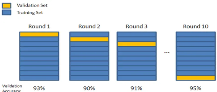
The models were evaluated using a leave-p-out cross validation. The principle of a leave-p-out cross validation is illustrated in Figure 7. This approach aims to use all the available samples of a ns-size dataset to assess the performance of a model, using
27 ns-p samples for calibration and p samples for validation and repeating the process until every sample has been used for both validation and calibration. The accuracy of classification of the model was evaluated using a performance score, usually de-fined as;
where 𝑎𝑎 is the accuracy of classification of the model, 𝑇𝑇𝑇𝑇 and 𝑇𝑇𝑇𝑇 are the number of true positives and true negatives, respectively, and 𝑛𝑛𝑠𝑠 is the total number of sam-ples of the database. By using all the samsam-ples for both training and validation, the risks of underfitting and overfitting the model are reduced (Berrar 2019; Drakos 2016).
2.4 Principal component analysis of the SKARA dataset
The external data with descriptive information was loaded into Evince to build a PCA model to evaluate the correlation of variables. The variables of interest in this analysis section are linked to the non-spectral information (external data). The var-iable “breed” was set as the categorical varvar-iable and a PCA was built. Score values were obtained for the observations and loading values for the variables.Figure 7 The principle of a leave-p-out cross validation, from Drakos, 2016
28
2.5 Image analysis
2.5.1 Supervised classification of pixels to train reference data
Figure 8 illustrates the workflow applied for the hyperspectral dataset.
Image analysis was made using the hyperspectral imaging software Breeze for both data sets, the hyperspectral images from Luleå and the RGB images from the SKARA dataset.
To train a supervised classification model, a dataset with reference data is required. In this study, no such reference data were available for either of the datasets. Here, the classification was supervised, meaning that the model is provided with mation about the classes of the samples used for classification. To obtain this infor-mation, a function was used in Breeze to manually select pixels of a specific consti-tution (e.g. protein, fat, etc.), adding those pixels to a user-defined class and create a reference dataset based on that selection. For each selected pixels, an average spectrum is calculated and added to the associated class. Hence the class and the spectral information for each class becomes the reference data that will be used to create a classification model. The selections were performed on the original images, choosing areas with known composition such as fat, protein etc.
29 Manual selection of grouped pixels can be limited, due to difficulty to select areas with pixels of a single class e.g. fat. To avoid this, the segmentation was set on representative spectra rather than on averaged ones. This method creates a number of user-defined points within the manual selection (in this case 10), where each point (i.e., pixel) gets its own spectral value. The spectrum of each selected pixels is then extracted and stored with its corresponding class. The spectral signature for each pixel is shown below in Figure 9.
The four classes used to build the PLS-DA model for the HS dataset were back-ground, plastic, fat and protein. For the SKARA dataset the two classes were fat and protein. The quantification was performed for the constituents fat and protein. For both the SKARA dataset and HS dataset, the reference data that were used for modelling the classification were split in a (i) calibration-validation (train dataset, approximately 50% of the reference dataset) and a (ii) test subset. The calibration-validation subset were used for training the model and then evaluate it by using the leave-p-out cross validation. The models classification accuracy were then esti-mated on the test subset.
2.5.2 Effect of plastic package
To evaluate the influence of the plastic on the classification, 40 images/ 20 samples (randomly chosen from the total of 120 samples) were loaded into Evince (Pred-iktera AB, Luleå). Evince is a software used to perform multivariate data analysis.
Figure 9 Spectral signature for a pixel of either (i) background, (ii) plastic, (iii) fat or (iv) protein. The pixels are extracted from the images in the HS dataset. The spectral information from the pixel and its corresponding class is used to train and test a classification model.
30
Each sample was imaged both with and without plastic. The predicted values for fat content and distribution (calculated by Breeze) were statistically analysed in Excel. Using a PCA model, the background was removed from the image. Then all the pixels from samples with plastic were selected and given a class variable; “with plastic”. The selection was inverted to mark the other group of pixels and classify it as “without plastic”. A PCA scatter plot was created and coloured based on the clas-ses (with or without plastic) to see how the samples clustered against each other. A PLS-DA model was then built to maximise the separation between the two classes 2.5.3 Analysis of fat distribution of both sides of the cut
In order to estimate if distribution of fat differed on either side of the sample, the samples were imaged on both sides of the cuts. The 40 images/ 20 samples that were used to evaluate effect of plastic package, were also used for this analysis. The beef sample were imaged on both sides, without plastic. The similarity of fat percentage and the distribution on both sides of the samples were analysed using the same method as for the evaluation of plastic package. Here the two classes were FRONT and BACK.
31
3.1 Correlation of the SKARA dataset variables
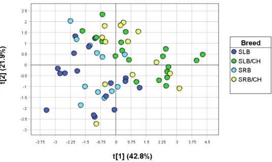
To evaluate how different variables in the external spreadsheet correlate, a PCA was performed using Evince (Figure 10). The figure shows that the two groups with cross breed steers clustered together and seem to be more alike. The purebred showed the same pattern. There was some overlapping from both groups indicating that there should be some individual differences affecting the results.
Variables of interest and their distribution are shown in Table 3. Figure 11 shows the correlation between the explanatory variables in the external spreadsheet (the variables appearing close to each other are highly correlated). It seems that carcass traits were correlated, but that marbling is equally related to both carcass trait and age. Age and fat class appear to be uncorrelated since they cluster on different sides of the chart.
A bi-plot was created to see how the different breeds correlated to the variables in the external spreadsheet (Figure 12). The results show that the crossbred steers tend to correlate more with the carcass traits and also have a higher live weight. The
3 Results
Figure 10 PCA score plot illustrating the correlation among the four breeds in the external spread-sheet from the SKARA dataset. It seems like the purebred breeds cluster and that the crossbred ani-mals are more similar.
32
purebred steers however tend to have more average fat and a higher marbling grade. The distribution of marbling grade among breeds is illustrated in Figure 13. The marbling was evaluated by an experienced grader.
Figure 11 PCA loading plot describing the correlation between the explanatory variables from the external spreadsheet from the SKARA dataset. Carcass traits seem to correlate.
Figure 12 Bi-plot of the SKARA dataset, showing how the scores correlate with the loadings. Scores that cluster close to a loading indicate correlation, the closer distance between the loading and the score the higher the correlation.
33
Figure 13 Violin boxplot describing the distribution of marbling grade among breeds in the SKARA dataset. The marbling grade was acquired manually by an experienced grader. The width of the plots represent the number of samples per class. The more samples in one class the wider the box-plot. The width of the violin describes the distribution of the samples for each class.
34
3.2
Training of pixel data for modelling classification and
quantification
3.2.1 RGB images
In the Breeze software, each representative spectra is referred to as a pixel. The classification matrix (Table 4-5) shows the total number of classified pixels for both the train and the test subsets. A classification matrix enables visualisation of the performance of the model. The matrix illustrates the pixels included of known “true” values and how often the model predicted the pixel class accurately. The classifica-tion model discriminated between fat and protein, showing a classificaclassifica-tion accuracy of 0.93 for fat and protein.
The PLS model used for quantifying fat showed a R2=0.95 which indicates a good performance of the model.
Table 4 Classification matrix for the train subset of the RGB classification model. The column ”To-tal” shows the amount of pixels with known (“true”) class included in the modelling. The matrix shows a classification accuracy of 99.5%. 1.7% of the fat pixels have been wrongly classified as pro-tein.
Classes Total Protein Fat
Protein 725 725 (100%) 0 (0%)
Fat 295 5 (1.7%) 290 (98.3%)
#Predicted 1020 (100%) Correctly 1015 (99.5%) Incorrectly 5 (0.5%)
Table 5 Classification matrix for the test subset of the RGB classification model. The matrix shows a classification accuracy of 95.5%. 7.3% of the protein pixel have been wrongly classified as fat.
Classes Total Protein Fat
Protein 495 459 (92.7%) 36 (7.3%)
Fat 313 0 (0%) 313 (100%)
#Predicted 808 (100%) Correctly 772 (95.5%) Incorrectly 36 (4,5%)
35 The distribution of fat content, predicted by Breeze, at different marbling grades is illustrated in Figure 14.
The boxplot indicates the minimum, the first, second and third quantile and the max-imum value of the group of sample.
3.2.2 Hyperspectral dataset
The number of pixels in each subset (train and test) for building the model and the outcome of classification are illustrated in Table 6-7. All pixels in both the train and test subsets were correctly classified (100%). The model performed classification with high accuracy for the four constituents with a classification accuracy 0.96 for fat, 0.95 for protein and 0.98 for background and plastic. The results indicate that the classification model performs well and accurately classifies the different con-stituents in the sample.
The PLS model used for quantifying the constituents showed a high R2=0.94, which indicates a good performance of the model.
Figure 14. Distribution at different marbling grades from subjective analysis and the average fat percentage predicted by Breeze from the RGB. The width of the boxplots represent the number of samples per class. The more samples in one class the wider the boxplot.
36
Table 6 Classification matrix for the train subset of the HS classification model. The matrix shows a classification accuracy of 100%.
Classes Total Bgr Plastic Protein Fat
Bgr 1851 1851 (100%) 0 (0%) 0 (0%) 0 (0%) Plastic 1018 0 (0%) 1018 (100%) 0 (0%) 0 (0%) Protein 1172 0 (0%) 0 (0%) 1172 (100%) 0 (0%) Fat 1433 0 (0%) 0 (0%) 0 (0%) 1433 (100%) #Predicted 5474 (100%) Correctly 5474 (100%) Incorrectly
Table 7 Classification matrix for the test subset of the HS classification model. The matrix shows a classification accuracy of 100%.
Classes Total Bgr Plastic Protein Fat
Bgr 1604 1604 (100%) 0 (0%) 0 (0%) 0 (0%) Plastic 946 0 (0%) 946 (100%) 0 (0%) 0 (0%) Protein 1586 0 (0%) 0 (0%) 1586 (100%) 0 (0%) Fat 912 0 (0%) 0 (0%) 0 (0%) 912 (100%) #Predicted 5048 (100%) Correctly 5048 (100%) Incorrectly
The spectral fingerprint for each pixel and its specific class is illustrated in Figure 9. When applying a PCA model on pixels of different classes, they cluster as shown in Figure 15. As shown in Figure 9, the constituents have unique spectral signatures. This is confirmed also in the PCA where the classes are separated based on their spectral differences. The clustering indicate that fat and protein are more similar in their spectral profile than plastic and background, yet they can be separated.
37 3.2.3 Effect of plastic package
When analysing the samples in Evince, the images with plastic do not differ from the images without plastic, as they do not cluster separately in the PCA scatter plot, but overlap. This indicates that the pixels in the samples with plastic are similar to those in the samples without plastic. Similar results were obtained with a PLS-DA model, indicating that the classes cannot be separated (Figure 16). Figure 17 illus-trates the comparison of the average fat % between the groups with and without plastic. The fat content was predicted by Breeze, using a quantification model. A 0.8 coefficient of determination was computed, indicating a high positive correla-tion between the two groups.
Figure 15 PCA model used to separate the pixels based on their spectral signature and class. It is shown that the four constituents cluster apart with fat and protein being the constituent with highest similarities.
38 y = 1,15x - 1,12, R² = 0,8 0 5 10 15 20 25 30 35 0 5 10 15 20 25 30 35 W ith p la st ic Without plastic Serie1 Linjär (Serie1) n = 20
Figure 17 Comparison of the calculated average fat content in samples imaged with and without plastic from the HS dataset, The scatter plot illustrating the linear correlation between calculated fat content for the group "with plastic package" and the group "without plastic package ". Figure 16 Samples from the hyperspectral dataset were used to analyse the average fat content when imaged with plastic package and without the plastic package. Evince was used to compare the pixels in the images, with and without plastic package. The pixels were classified as either with or without plastic. A PLS-DA model was used to separate the two classes of pixels belonging to either WITH plastic or WITHOUT plastic. The green colour represent the pixels WITH plastic and the blue colour represents the pixels WITHOUT plastic. The two classes overlap, indicating little difference between the pixels in both classes.
39 3.2.4 Analysis of fat distribution of both sides of the cut
The PLS-DA model indicate that the pixels in the FRONT class cannot be separated from the pixels in the class BACK (Figure 18). It seems that the distribution and fat content are similar for both the front and back sides.
When including all 40 images, the result indicate that the distributions of the pixels are similar for both the front and backside. However, when selecting and classifying pixels of fat and protein respectively, it is shown that the amount and distribution of fat differs within pair of samples (Figure 19). These results indicate that there might be some biases in the PLS-DA model when the pixels are classified as a group and compared against several samples, which do not correlate with each other.
Figure 18 Samples from the hyperspectral dataset were used to analyse the distribution of fat on both sides of the sample. Evince was used to compare the imaged front and backside, by classify the pixels as FRONT or BACK. A PLS-DA model was used to separate the two pixel groups. The green colour represent the pixels BACK and the blue colour represents the pixels FRONT. The two classes overlap, indicating little difference between the pixels in both classes.
40
Figure 20 and figure 21 show the average fat content and the fat distribution values, calculated by Breeze for both BACK and FRONT. The linear scatterplot show a low coefficient of correlation between both fat content and fat distribution, indicating that the streaks of fat does not follows throughout the whole sample. This is con-firmed when paired samples are compared, as the amount and distribution of fat is different between front and side in the majority of the samples (Figure 19).
Figure 19 Merge of samples imaged from front and back side of the beef cuts in the HS dataset. Fat is marked as green. The red marker indicate front samples. The green square indicted a pair of samples with the front side sample above the back side sample. This is equal for all samples in the merged image. The image indicate that fat content and distribution differs between front and back.
41
y = 0,74x + 5,83, R² = 0,53
0,0 5,0 10,0 15,0 20,0 25,0 30,0 0,0 10,0 20,0 30,0 FRO NT BACK Serie1 Linjär (Serie1) n = 20Figure 20 Comparison of the calculated average fat content in samples imaged from both sides of the sample from the HS dataset. The scatter plot illustrating the linear correlation between calcu-lated fat content for the group "FRONT " and the group "BACK".
y = 0,68x + 5,43, R² = 0,43 0 5 10 15 20 25 0 5 10 15 20 25 BAC K FRONT Serie1 Linjär (Serie1) n = 20
Figure 21 Comparison of the calculated fat distribution in samples imaged from both sides of the sample from the HS dataset. The scatter plot illustrating the linear correlation between calculated distribution for the group "FRONT " and the group "BACK".
42
3.3 Comparison of objective fat analysis and subjective
marbling grading
The objective average fat % was compared to a subjective grading of the marbling for each sample. The subjective grading was performed by the same experienced grader who graded the beef samples in the SKARA dataset.
A violin-boxplot shows the distribution of the predicted fat content at different mar-bling levels. The figure indicates that marmar-bling grade seem to increase with higher fat content. However, the fat content varies within class and also different grades get the same fat content. To see how the marbling value (subjective), fat distribution % and average fat % correlated the numbers were transferred to a spreadsheet and then loaded into Evince. A PCA model was applied to show the clustering of the three variables (Figure 23). Fat percentage and fat distribution seem to be highly connected, while the subjective grading and the other traits are negatively corre-lated.
Figure 22 The average fat percentage predicted by Breeze for the HS dataset was compared to the marbling grade, which was acquired visually (subjectively) by an experience grader. It seems like higher marbling grade is correlated with higher fat percentage. Violin boxplots shows the distribution between the objectively predicted fat % and the subjectively analysed marbling. The width of the box-plots represent the number of samples per class. The more samples in one class the wider the boxplot. The width of the violin describes the distribution of the samples for each class.
43 3.3.1 Comparison of the accuracy between RGB image and HS image
based analysis
Comparing the classification accuracy, the model based on HS images showed bet-ter performance with no incorrect classification. For the RGB image dataset, 4.5% of the pixels in the test subset and 0.5% in the training subset were classified wrong. The quantification model for the RGB images resulted in a R2=0.95, and of 0.94 for the HSI. However, for the RGB images the results show some odd outcomes where some samples with no fat get high values and some samples get negative values, even though they have visible fat streaks. The fat values and distribution for the HS dataset are much more consistent with the sample images.
Figure 23 PCA loading plot, showing the relationships of the subjectively analysed marbling grade and the fat distribution and fat percentage predicted by Breeze for the HS dataset. Distribution and fat content are clearly clustered.
44
4.1 Intercorrelation of the SKARA dataset variables
According to the PCA loading plot, marbling seems to correlate with distribution and average fat. A high fat proportion together with a low distribution should not generate a good marbling grade, since the marbling depends on both amount and homogenous distribution of fat in the meat cut (Velásquez et al. 2017; Xiong et al. 2014). With that in mind it is positive that marbling and distribution seem to have a high correlation and also that it connects with the fat percentage.
For the carcass traits; (i) fat class, (ii) form class, (iii) carcass ratio and (iv) carcass weight, there is a high correlation between them all except for the fat class. In this study, approx. half of the dairy animals were crossbred with a later maturing breed. Those breeds, in general, receives a higher form class than the early maturing breeds and dairy breeds. They also put on less fat and gain a lower fat class. It is therefore expected that they receive a higher form class and also higher carcass weight and carcass ratio (Albertí et al. 2008; Clarke et al. 2009).
Marbling did correlate with age, which has been found in earlier studies (Albrecht et al. 2006; Venkata et al. 2015). The animal will deposit fat in the muscle last, therefore the older the animal gets, the more likely it is that it gets a high marbling grade. Also the dairy breeds SLB and SRB generated the highest marbling grades in general. It should be expected since they are growing older before slaughtered, and thus have the time to deposit fat into the muscles (Albrecht et al. 2006; Venkata et al. 2015). They are also maturing earlier, putting on more fat compared to the crossbred steers. The crossbred steers are influenced by the late maturing beef breed and should be leaner, with higher carcass ratio (Pfuhl et al. 2007). However, the diversity in marbling among the breeds are not high, so it cannot be concluded that the differences are caused only by breed. The differences within each breed does indicate that there are individual traits that affect the marbling grade as much as breed, age and sex.
45
4.2
Classification and quantification of the meat
components
4.2.1 SKARA dataset
When evaluating the classification, the RBG model performs the classification of constituents with high accuracy.
However, there are some problems finding the small streaks of intramuscular fat in the samples. It seems that the majority of the surface has been classified as protein, even though it by eye is possible to see the intramuscular fat. This indicates that the small areas of fat have been misclassified as protein pixels.
The pixels that were derived from the manual selection were randomly chosen by the software. When selecting those small areas of intramuscular fat, it is possible that pixels from both fat and protein have been mixed. When the whole selection is divided into 10 pixels, it is probable that some of them belonged to protein when classified as fat. The class “fat” would then include pixels with spectral values from both pure fat, but also protein. This could be an explanation of why the model have had problems classifying the narrow streaks of intramuscular fat in the cuts. When quantifying the amount of fat in the cuts, the prediction of average fat per-centage in also indicate some unrealistic results. The average fat perper-centage of the surface values shows unexpected high numbers, e.g. measurements indicating ap-prox. 20% fat, which is unlikely to be true when analysing the sample by eye. How-ever, the images having the most unreliable results also seem to have been photo-graphed with another light settings. The badly quantified images appear much brighter in colour compared to samples that have been given more likely fat values. The different light settings when taking the images may cause the misclassification, due to colour differences among pixels with the same class.
The high average fat values are still questionable – however they are likely to be caused by the fat cap and bigger lumps of fat that are still left in some images. These factors will cause overestimated values for the average fat % and also the distribution, resulting in a poor correlation with the subjective marbling estimation. The lowest marbling grade (1) includes predictions that have the same average fat % as marbling grade 3. Since marbling level increase with higher fat content (Lucherk et al. 2016), a lower marbling grade should contain less fat. This is con-sistent for all levels of marbling.