Master Thesis
HALMSTAD
UNIVERSITY
120
Human Understandable Interpretation of
Deep Neural Networks Decisions Using
Generative Models
Embedded and Intelligent Systems, 30
credits
Halmstad 2019-11-26
Abdallah Alabdallah
Abdallah Alabdallah: Thesis Report, Human Understandable Interpre-tation of Deep Neural Networks Decisions Using Generative Models,
c
November 2019 s u p e r v i s o r s: Cristofer Englund Sepideh Pashami
A B S T R A C T
Deep Neural Networks have long been considered black box systems, where their interpretability is a concern when applied in safety crit-ical systems. In this work, a novel approach of interpreting the de-cisions of DNNs is proposed. The approach depends on exploiting generative models and the interpretability of their latent space. Three methods for ranking features are explored, two of which depend on sensitivity analysis, and the third one depends on Random Forest model. The Random Forest model was the most successful to rank the features, given its accuracy and inherent interpretability.
C O N T E N T S
1 i n t r o d u c t i o n 1
2 r e l at e d w o r k 3
3 m e t h o d 5
3.1 Dataset Description 6
3.2 Disentangled Features extraction 6
3.3 The Discriminator Model 8
3.4 Discriminator Interpretability 8
3.4.1 Generated Images 10
3.4.2 Original Images 11
3.4.3 Random Forest 12
4 r e s u lt s 15
4.1 Disentangled Features extraction 15
4.1.1 Structures and Hyperparameters Tuning 15
4.1.2 Final Generative Model 18
4.1.3 Final Learned Features 19
4.2 The Discriminator Model 20
4.3 Discriminator Interpretability 21 4.3.1 Generated Images 21 4.3.2 Original Images 23 4.3.3 Random Forest 23 5 d i s c u s s i o n a n d c o n c l u s i o n 32 b i b l i o g r a p h y 34 iii
L I S T O F F I G U R E S
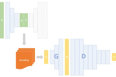
Figure 1 Generator G, Discriminator D, and Latent dis-tribution (µ,Σ). 5
Figure 2 Samples of Pride 2011 dataset 7
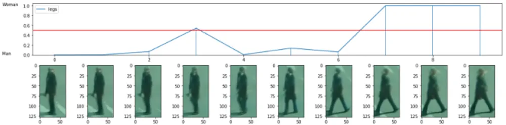
Figure 3 Changes of discriminator response on travers-ing the "Leg Separation" feature. 10
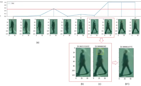
Figure 4 (a)-Changes of discriminator response on travers-ing the "Leg Separation" feature. (b),(c) and (b1) comparison between two generated images 11
Figure 5 Using multiple images at every point on the z axis, and averaging the decision score of the discriminator. 12
Figure 6 Extracting the z (disentangled features) using the generator (G), and extracting the discrim-inator (D) decision y of the training dataset x, and preparing the data for the Random Forest model. 13
Figure 7 Generated images from all models 16
Figure 8 Size of person and brightness of clothes entan-gled features, learned by model S2. 16
Figure 9 Reconstruction of samples of test images by the small structure 17
Figure 10 Reconstruction of samples of test images by the medium structure 18
Figure 11 Reconstruction of samples of test images by the large structure 19
Figure 12 Legs sepatation 20
Figure 13 Front View Angle 21
Figure 14 Back View Angle 23
Figure 15 Jacket Length 24
Figure 16 Clothes Brightness 26
Figure 17 Person Size - This feature is sometimes entan-gled with clothes brightness 27
Figure 18 Example of three features, comparing the gen-erated images quality between the regular train-ing method (first line of each feature), and the new method suggested in [2] (second line of
each feature) 28
List of Figures v
Figure 19 Example of the reconstruction of images from the test set, comparing the original images, the reconstructed images with new training method suggested by suggested in [2], and the
recon-structed images with the old training method 28
Figure 20 Every line contains images generated by vary-ing only the respective feature on the left. In-terpretations are in Table10. The names of the
features corresponds to the indexes of the vari-ables in the generative model, and have no mean-ing 29
Figure 21 Training and validation accuracy and loss of the discriminator model. The model achieved training Accuracy 1.0 and validation accuracy is 0.9999, with training loss 1.4e − 4 and vali-dation loss 5.5e − 4 30
Figure 22 Responses of the discriminator on generated images with respect to each feature 30
Figure 23 Responses of the discriminator on the original images with respect to each feature, consider-ing the mean value of the responses at each location 30
Figure 24 Grid search for number of estimators hyper-parameter, where 185 estimators achieved the best score of 97.7% training accuracy and 98.4% testing accuracy 31
L I S T O F TA B L E S
Table 1 Dataset Description. 6
Table 2 The details of the seven trained models, with three small, medium and large structures and multiple hyperparameters. z is the capacity of the latent variables, beta is the weight of the KL divergence term, and BN is Bach normal-ization. 9
Table 3 The Discriminator structure. 10
Table 4 The latent variables for every image in the train-ing data discretized into 13 bins, along with discriminator response ydfor each image. 12
Table 5 The latent variables for every image in the train-ing data, along with the discriminator response. 14
Table 6 Training details of the seven generative mod-els. 15
Table 7 Reconstruction Normalized Mean absolute er-ror NMAE. 17
Table 8 Disentangled features learned by the seven ex-perimental models 18
Table 9 Number of Used Variables of the latent space for each model 19
Table 10 Interpretations of features shown in Figure20,
along with confidence in the interpretation 22
Table 11 Features ranked by their importance based on the generated images method 22
Table 12 Features ranked by their importance based on the original images method 25
Table 13 Features ranked by their importance based on the random forest method 25
A C R O N Y M S
DNN Deep Neural Network
CNN Convolutional Neural Network
VAE Variational Auto-Encoder
GAN Generative Adversarial Networks
MDI Mean Decrease Impurity
MAE Mean absolute error
ELBO evidence lower bound
1
I N T R O D U C T I O N
Deep Neural Networks DNNs have achieved state of the art results in various domains, and it started to be used in many problems, es-pecially in image recognition tasks [10], [16]. DNNs learn to classify
input through successive application of linear and non-linear opera-tions until they reach to a certain decision.
Images are very high dimensional objects. They contain both rel-evant and irrelrel-evant information buried in noise. To automatically extract features from images, a special type of DNNs called Convolu-tional Neural Networks (CNNs) is used. They proved to be powerful tools to extract relevant information using very complicated struc-tures consisting of convolutional layers, pooling layers, and millions of parameters. On the other hand, the high dimensionality of their in-put and the complexity of their structure, made the task of explaining why the network reached a decision, a challenging task.
Nowadays, DNNs are being used in different kinds of systems, but concerns arise when they are used in systems where safety is critical, like medical diagnoses, autonomous vehicles [14]. In such systems,
decisions must be interpretable.
In this work, the issue of interpretability of DNNs is addressed, focusing on CNNs, by answering the questions,
• What are the salient features in images, which the CNN utilizes in decision making?
• How much is the importance of each feature?
Most of the existing solutions try to explain the decision of the CNN using the input pixel space, either by backpropagating the acti-vation of the final layer to the input space and building saliency maps, or by constructing image that maximally activates a certain output.
Pixel Space is a very high dimensional space, where the pixels are the axes of this space. Changes of a single pixel on its own, is not meaningful, where objects or concepts in images usually comprise sets of pixels. Those pixels are the result of rendering (or hypothetical rendering in the case of real images) of lower dimensional factors, called the generative factors, like the position, the size or the color of the object in the image. Variations in generative factors can cause changes in CNN decisions, which methods that use pixel space for explanation, may not be able to consider. However, to account for the variations of the generative factors of a dataset in the explanation of the CNN decisions, those factors should be extracted first.
i n t r o d u c t i o n 2
Generative factors of a dataset can be extracted manually, by label-ing each image in the dataset with values representlabel-ing the respective generative factors’ variations. One example is in [19], where they
man-ually labeled a dataset of pedestrians based on their skin tones. The purpose of their study is to investigate the effect of the skin tone of pedestrians,which is one of the generative factors, on the performance of state of the art pedestrian detection systems. They found out that there is a predictive inequality in these pedestrian detection systems based on the skin tones of pedestrians, which revealed a bias in the dataset. In fact, they discovered that the reason for this predictive in-equality is that the training dataset contains more than three times as many images of light skinned pedestrians compared to dark skinned pedestrians.
Nevertheless, in order to study the effect of all the generative fac-tors of a dataset, it is almost impossible to manually label all im-ages with all their respective generative factors. Fortunately, genera-tive models that learn disentangled representation like β-Variational Autoencoders [5], are able to discover and map each of the generative
factors of a dataset to a variable in its latent space.
In this work, a novel approach is proposed, by explaining the de-cision of the CNN using the interpretable latent space of the dataset, utilizing the disentanglement power of β-Variational Autoencoder model. The case of a binary classifier is used, and the features in im-ages that help the network to distinguish between the two classes are extracted and ranked. Three method for ranking the features, based on their importance in the decision, are explored.
2
R E L AT E D W O R K
Previous researches have addressed the interpretability issue of DNNs from different points of view, all of which, depend on visualization as an interpretation. Four main methods exist that focus on visualizing different aspects of CNNs features and mechanisms, namely Activa-tion MaximizaActiva-tion, DeconvoluActiva-tional Networks (DeconNet), Network Inversion, and Saliency Maps.
In an early work [17], they tried two gradient-based techniques of
visualization. The first one is based on Activation Maximization and focuses on visualizing the class model learned by the the CNN. They synthesized an image I∗ that maximizes the activation of a certain class Sc as shown in Eq.1.
I∗ = argmaxISc(I) − λ||I||22 (1)
Were λ is the parameter of the L2-Norm regularization. This method
blurry images of the class patterns.
The second technique in [17] focuses on Image-Specific Class Saliency.
This technique is based on computing the gradient of the class score Sc with respect to the input I. However, because the score is a
nonlin-ear function, this is done by computing the first-order Taylor expan-sion at point (image) I0 as shown in Eq.2.
w = ∂Sc
∂I |I0 (2)
Where w represents the contribution of the pixels in the score Sc,
which allows to highlight the pixels in the input image based on their contribution.
In more recent work [13] based on Activation Maximization, they
utilized a deep generator network to synthesize real-like images that highly activate neurons. Instead of the L2-Norm regularization in [17],
this method, by using a generator network, enforces a real image prior. This will help produce real-like images rather than blurry pat-terns as in [17].
In [20] they used Deconvolutional Networks [21], to map internal
features activations back to the input space. This will show the pat-terns in the image that activated a certain neuron.
In [12], they utilized Network Inversion to reconstruct the image
from different layers in the network. They formulated the problem as an optimization problem, where they search for the image whose representation best matches the one in the layer in consideration. This method gives insight into the information captured by each layer.
r e l at e d w o r k 4
In the most recent work [4] which falls under Saliency Maps
meth-ods, they built a causal model based on salient concepts in the im-age. Instead of working on the level of pixels, they embedded Auto-Encoders between the layers to extract higher level concepts. By mak-ing interventions on these concepts, they measured the causal effect of each concept on the output of the network. Finally, they visualized these concepts on the image based on their effect.
Another topic that is related to interpretability is Disentanglement of Representation. It is one of the generic priors of representation learning first proposed by Yoshua Bengio in [1]. Disentanglement
of representation is an important property when it comes to inter-pretability of the latent space features. In a disentangled representa-tion, each latent variable represents one direction of variation. Many works addressed disentanglement and it is still an active field of study.
In [5] a β-VAE model was proposed. It is based on the Variational
Auto-Encoder (VAE) framework [9] where they added a
hyperparam-eter β to control the pressure on the latent distribution to match a unit Gaussian. Increasing the β value, increases the pressure towards learning disentangled features, but it affects the reconstruction qual-ity.
FactorVAE is another model based on VAE proposed in [7]. It
en-courages the latent distribution to match the product of its factors, hence uncorrelated, without compromising reconstruction quality.
On the other hand, in [3], based on Generative Adversarial
Net-works (GANs), InfoGAN model was proposed. A regular GAN model, uses an input noise vector z, where no restrictions are imposed. This might lead the network to use the z vector in an entangled manner. InfoGAN, splits the input vector into two parts. The noise source z and latent code c. By assuming that the code c is factorized (i.e. P(c1, c2, . . . , cL) =
QL
i=1P(ci)), and by maximizing the mutual
infor-mation between c and the constructed image, it will learn disentan-gled features of images.
Visualization is a good approach for interpretability. It helps in un-derstanding the patterns for which the internal neurons are looking, and highlighting the important areas in images that contributed in the decision. On the other hand, visualization does tell anything about the variations of features in images, and does not show the effect of these variations on the decision of the DNN. Variations are changes generative factors in images. Studying variations can reveal biases in DNNs decisions as in [19] where they studied the effect of variation
in skin tone on state-of-the-art pedestrian detection systems. They found that the studied systems are biased and better in recognizing light skinned vs. dark skinned people. Discovering such kinds of bi-ases is very important when it comes to safety critical systems.
3
M E T H O D
In this thesis, we exploit the interpretability power of disentangled features to explain the decision of CNNs. Figure1shows the overall
structure of the system that consists of a generator G and a discrim-inator D. The generator G is the part of the system that we use to extract and interpret features from images, that will help to explain the mechanism in which the discriminator D is making decisions. G is a β-Variational Auto-Encoder that learns disentangled latent features, and D is a CNN with binary output representing two classes.
The generator G is trained on pedestrian images X, were it learned disentangled features z normally distributed with (µ,Σ). These fea-tures represent the axes of variations in the training dataset X, like the length of the jacket, and brightness of the clothes . . . etc. The gen-erator is used to generate images along each axis in order to infer the generative factors represented by each latent feature, then a meaning-ful label is assigned to each feature as shown in Section3.2.
The discriminator D is also trained, on the same dataset X (after labeling with two classes). The goal of this work is to discover and rank the features that the discriminator D takes into account in its decision.
Three ways are explored for ranking feature importance as de-scribed in Section 3.4. The assigned meaningful labels to the latent
features, along with their importance ranking, are our proposed in-terpretation of the discriminator decisions.
Figure 1: Generator G, Discriminator D, and Latent distribution (µ,Σ).
3.1 dataset description 6
Table 1: Dataset Description.
Women Men Number of Persons 442 457
Number of Images 49344 44054 Number of Training Images 38000 35000 Number of Validation Images 7000 6000
Number of Testing Images 4344 3054
3.1 d ata s e t d e s c r i p t i o n
Person Re-ID (PRID) Dataset 2011 [6] is used to train the models. The
dataset contains around 95000 (128x64) RGB images as sequences of walking persons extracted from two static surveillance cameras. The number of persons is 475 in one view and 865 from the other with 245persons appear in both cameras.
Our initial idea was to train a discriminator that distinguishes be-tween pedestrians and not pedestrians, but due to our choice of the dataset, it was hard to find challenging negative examples to train the discriminator. As a result, it was very easy for the discriminator to distinguish between positive and negative examples as they have very different distributions. To overcome this issue, we changed the problem from pedestrian classification, to women verses men classifi-cation, where we can separate the dataset into two classes "Woman" and "Man".
For training the generator, the dataset is divided into 85000 images as training set, 5000 images as validation set and 5000 images as test set. Horizontal flip augmentation is applied to increase the number of samples.
For training the discriminator, the data is labeled with 1 and 0 representing a woman, and a man respectively. The dataset contains almost equal numbers of women and men with 442 women (49344 images) and 457 men (44054 images). The dataset is divided into training, validation, and test sets as shown in Table 1 This dataset
is selected for this work, due to the relatively large number of im-ages, and that the images show people from different angles and in multiple positions, things that will help the network to learn multi-ple factors of variations. Figure2 shows samples of images from the
dataset.
3.2 d i s e n ta n g l e d f e at u r e s e x t r a c t i o n
In this work, β-Variational Auto-Encoder (β-VAE) [5] is used as a
generative model. It is based on the framework of Variation Auto-Encoder (VAE) [9], which learns disentangled latent features by
en-3.2 disentangled features extraction 7
Figure 2: Samples of Pride 2011 dataset
couraging the approximate posterior distribution q(z|x) to match a standard Gaussian distribution prior p(z). The objective function of β-VAE Eq.3matches the objective function of VAE with extra weight
on the KL-Divergence term to enforce more disentanglement.
L(θ, φ, x, z) = Eqθ(z|x)[logpθ(x|z)] − βDKL(qφ(z|x)||p(z)) (3)
Learning the right structure and hyperparameters of the network is a hard and time-consuming task. Starting by exploring different hy-perparameters, a suitable activation function and optimization method are found. Leaky-Relu activation with 0.01 leak, and Adam optimiza-tion method [8] are used. Inspired by the structure used in [5], three
different sizes of structures are experimented. The structures range from small, medium, to large, named in Table2 with their initials S,
M, and L respectively. For each structure, different values of the β hyperparameter are experimented to find the suitable value which achieves the best disentanglement with a good reconstruction quality. Moreover, different number of latent variables for some structures are also experimented. Due to the long training time, it was not possible to try all values of hyperparameters for all models. Table 2 contains
3.3 the discriminator model 8
Studying the seven structures in Table 2, structure M3 is selected,
as it learned the largest number of features and it has the best re-construction among other structures based on the mean absolute er-ror (mae) between the original and the reconstructed images. The selected model is retrained, following the method suggested by [2] to
enhance reconstruction quality. They suggested to start with a large weight on the KL-Divergence term in the early stages of training to force the features to be disentangled, then reduce the weight gradu-ally to allow for a better reconstruction. The new objective function Eq.4 contains a new term C by which it can control the value of the
KL-Divergence term. The model is trained with C = 0 for 100 epochs, then gradually the C value is increased up to 100.
L(θ, φ, x, z, C) = Eqθ(z|x)[logpθ(x|z)] − β|DKL(qφ(z|x)||p(z)) − C| (4)
3.3 t h e d i s c r i m i nat o r m o d e l
The discriminator is the target system to be explained. In our case, the discriminator job is to distinguish between women and men. The assumption is that the we have access to the dataset on which the discriminator is trained, which means that the generator G will be trained on the same dataset as the discriminator. For the discrimina-tor, similar structure to the encoder part of the "Medium" structure in Table 2 is followed, as it is the model that is selected for the
gen-erator, and showed a good behavior in fitting the data. Table3shows
the detailed structure of the discriminator. The output of the model is a logistic function where 1 represents the "Woman" class and 0 rep-resents the "Man" class. The discriminator model was trained using default "Adam" optimization method, with early stopping after 100 epochs of no improvement.
3.4 d i s c r i m i nat o r i n t e r p r e ta b i l i t y
This section focuses on explaining how the CNN reaches its decision, in other words, it measures the effect of each of the extracted features Z on the decision of the neural network, in order to rank the fea-tures based on their importance. Three methods are used to measure the importance of the features. In the first two methods, controlled input is used, by generating images subject to changing one latent variable at a time, see Section3.4.1, or by using the training dataset
and measuring the average response of the discriminator along one axis (latent variable) at a time, see Section3.4.2. In the third method,
the explainability power of a Random Forest model is exploited, see Section3.4.3.
3.4 discriminator interpretability 9
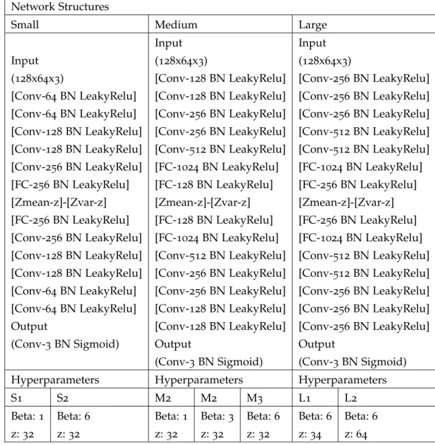
Table 2: The details of the seven trained models, with three small, medium and large structures and multiple hyperparameters. z is the capacity of the latent variables, beta is the weight of the KL divergence term, and BN is Bach normalization.
Network Structures
Small Medium Large
Input (128x64x3) [Conv-64 BN LeakyRelu] [Conv-64 BN LeakyRelu] [Conv-128 BN LeakyRelu] [Conv-128 BN LeakyRelu] [Conv-256 BN LeakyRelu] [FC-256 BN LeakyRelu] [Zmean-z]-[Zvar-z] [FC-256 BN LeakyRelu] [Conv-256 BN LeakyRelu] [Conv-128 BN LeakyRelu] [Conv-128 BN LeakyRelu] [Conv-64 BN LeakyRelu] [Conv-64 BN LeakyRelu] Output (Conv-3 BN Sigmoid) Input (128x64x3) [Conv-128 BN LeakyRelu] [Conv-128 BN LeakyRelu] [Conv-256 BN LeakyRelu] [Conv-256 BN LeakyRelu] [Conv-512 BN LeakyRelu] [FC-1024 BN LeakyRelu] [FC-128 BN LeakyRelu] [Zmean-z]-[Zvar-z] [FC-128 BN LeakyRelu] [FC-1024 BN LeakyRelu] [Conv-512 BN LeakyRelu] [Conv-256 BN LeakyRelu] [Conv-256 BN LeakyRelu] [Conv-128 BN LeakyRelu] [Conv-128 BN LeakyRelu] Output (Conv-3 BN Sigmoid) Input (128x64x3) [Conv-256 BN LeakyRelu] [Conv-256 BN LeakyRelu] [Conv-256 BN LeakyRelu] [Conv-512 BN LeakyRelu] [Conv-512 BN LeakyRelu] [FC-1024 BN LeakyRelu] [FC-256 BN LeakyRelu] [Zmean-z]-[Zvar-z] [FC-256 BN LeakyRelu] [FC-1024 BN LeakyRelu] [Conv-512 BN LeakyRelu] [Conv-512 BN LeakyRelu] [Conv-256 BN LeakyRelu] [Conv-256 BN LeakyRelu] [Conv-256 BN LeakyRelu] Output (Conv-3 BN Sigmoid) Hyperparameters Hyperparameters Hyperparameters
S1 S2 M2 M2 M3 L1 L2 Beta: 1 z: 32 Beta: 6 z: 32 Beta: 1 z: 32 Beta: 3 z: 32 Beta: 6 z: 32 Beta: 6 z: 34 Beta: 6 z: 64
3.4 discriminator interpretability 10
Table 3: The Discriminator structure.
Discriminator Structure Input (128x64x3) [Conv-128 BN LeakyRelu] [Conv-128 BN LeakyRelu] [Conv-256 BN LeakyRelu] [Conv-256 BN LeakyRelu] [Conv-512 BN LeakyRelu] [FC-512 BN LeakyRelu] [FC-64 BN LeakyRelu] [FC-1 BM Sigmoid] 3.4.1 Generated Images
The initial idea of this work is to use controlled input to measure the sensitivity of the target system (the discriminator) to the variations along each axis (latent feature). The generator is used to generate 10 images along each axis of variation, by setting all the latent features to 0 except one, and vary the later from −3 to +3 (where all features are normally distributed). The 10 images are then presented to the discriminator, and the response for each image is recorded. By re-peating this for all the latent variables and measuring the variance of the discriminator responses for each variable, we rank the latent variables based on their importance. The feature importance is based on the response variance, assuming that the feature that causes the discriminator response to vary more, plays a more important role in the discrimination. Moreover, it is one of the sensitivity analysis tech-niques [15], that is used to measure features importance in non-linear
systems. Figure 3 shows an example of the discriminator response
changes on traversing the "Legs Separation" feature.
Figure 3: Changes of discriminator response on traversing the "Leg Separa-tion" feature.
Unfortunately, this method has a drawback. Because it is dealing with real images, the generated images along one axis of variation, al-lows for other smaller variations in images, that could be important to
3.4 discriminator interpretability 11
the decision. As an example of those small variations, Figure4shows
a comparison between two images along the axis of "Legs separation" feature, where the discriminator changes its decision from "Man" to "Woman", while intuitively it should not. In order to discover the part of the image that causes this big change, different crops from image (c) to image (b) are copied. Image (b1) is the result of copying the head from image (c) and paste it on image (b). We notice that the small variations in the head area between images (b) and (c) is the responsible of changing the decision from 0.0621 (where 0 represents the class Man) to 0.9999 (where 1 represents the class Woman).
Figure 4: (a)-Changes of discriminator response on traversing the "Leg Sepa-ration" feature. (b),(c) and (b1) comparison between two generated images
3.4.2 Original Images
To overcome the drawback of the previous method described in Sec-tion3.4.1, it is reasonable to use multiple images at every point along
the latent variable axis, and averaging the responses of the discrimina-tor for the respective images. Doing so, reduces the effect of the small variations and keeps the effect of the original variation of the latent variable at consideration. Instead of generating images, the original dataset is used. The zi features are extracted for every image xi. On
parallel, all images are presented to the discriminator of which the re-sponse ydi is recorded for each image. In order to align images with
similar z values, where z variables are continuous, the z variables are discretized into 13 bins b ∈ (−3, −2.5, −2, −1.5, −1, −0.5, 0, 0.5, 1, 1.5, 2, 2.5, 3) as in Table 4. By doing so, it is possible to average the values of the
responses in each bin, where bins represent discrete locations along the z axes. The expected value Rbdefined in Eq.5, at each location b
3.4 discriminator interpretability 12
Table 4: The latent variables for every image in the training data discretized into 13 bins, along with discriminator response yd for each image.
z0 z1 z3 ... z31 yd 0 -2 0 ... -0.5 0.98 0.5 0 -3 ... 1 0.002
-1 -1.5 2 ... 0.5 0.001
on z axis, represents the average response of the discriminator at the respective location,
Rb= E(i∈S)[dyi] (5)
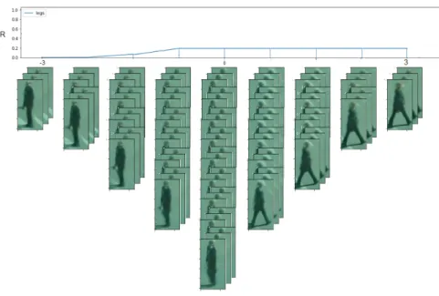
Where S is the set if images at the respective b location. This should in-dicate wither the discriminator response at the respective location, is biased towards women or men, and will allow measuring the changes of the discriminator responses along the respective axis. To exclude extreme location where fewer images exist as shown in Figure5, only
values between (−2, 2) are considered. As in Section 3.4.1, the
vari-ance of R of each latent variable is considered to represent the impor-tance of the respective variable.
Figure 5: Using multiple images at every point on the z axis, and averaging the decision score of the discriminator.
3.4.3 Random Forest
Random Forests are powerful models that rely on the concept of en-semble learning. A Random Forest, consisting of multiple Decision Trees, derives its interpretability from the interpretability of Decision
3.4 discriminator interpretability 13
Tree models. It is possible to calculate features importance using the Mean Decrease Impurity (MDI) measure [11]. For an input feature
zi, the importance Eq. 6is calculated as the summation of weighted
impurity decreases ∆i for all nodes t where the feature zi is used,
averaged over all the trees EnT in the ensemble.
Imp(zi) = E(T∈En
T)[
X
t∈T :v(t)=zi
p(t)∆i(t)] (6)
Where p(t) is the probability of reaching the node t, and v(t) is the variable used in node t.
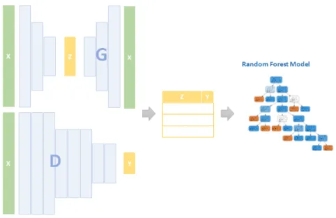
In this method, the problem is converted into a regular machine learning problem. Figure6is an illustration of this process. We extract
the latent features z for all images and record the responses of the discriminator ydfor respective images. The extracted features, along
with their respective discriminator response ydare stacked as in Table
5.
A Random Forest model is fitted to this data, where the indepen-dent variables are features extracted from images, and the depenindepen-dent variable is the discriminator response yd. By doing so, the Random
Forest model captures the behavior of the discriminator. Based on the features importance of this model, it is possible to gain insight into the features on which the discriminator depends.
Figure 6: Extracting the z (disentangled features) using the generator (G), and extracting the discriminator (D) decision y of the training dataset x, and preparing the data for the Random Forest model.
3.4 discriminator interpretability 14
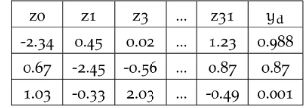
Table 5: The latent variables for every image in the training data, along with the discriminator response.
z0 z1 z3 ... z31 yd
-2.34 0.45 0.02 ... 1.23 0.988 0.67 -2.45 -0.56 ... 0.87 0.87 1.03 -0.33 2.03 ... -0.49 0.001
4
R E S U LT S
4.1 d i s e n ta n g l e d f e at u r e s e x t r a c t i o n
4.1.1 Structures and Hyperparameters Tuning
Seven models of similar structures with increased width from small, medium to large, were trained. The purpose is to test the effect of increasing the width on the reconstruction quality. The intuition be-hind that is trying to capture more information in the first layers, that might be lost when using the smaller model. It was supposed that the effect of increasing β hyperparameter value, to be tested for all of the structures, but unfortunately, due to long training time, it was only possible to test a limited number of β values. As shown in Ta-ble2, the small structure was tested with two β values 1 and 6, the
medium structure was tested with three β values 1, 3 and 6, and the large structures was tested with only one β value 6, but varying the latent variables capacity 34 and 64.
The models were trained with Adam optimization method, apply-ing early stoppapply-ing after 50 epochs of no improvement in the valida-tion loss. Table6includes training details for all the models.
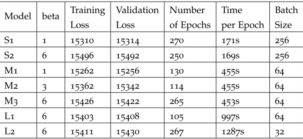
Table 6clearly shows that increasing the beta value, increases the
loss, which complies with the fact that increasing the weight on the KL divergence term deceases the evidence lower bound (ELBO) of the likelihood. The generated images, as expected, showed that increas-ing the β value will result in blurrier images with more disentangled features, and decreasing it will result sharper images with entangled features.
Table 6: Training details of the seven generative models.
Model beta Training Loss Validation Loss Number of Epochs Time per Epoch Batch Size S1 1 15310 15314 270 171s 256 S2 6 15496 15492 250 169s 256 M1 1 15262 15256 130 455s 64 M2 3 15362 15342 114 455s 64 M3 6 15426 15422 265 453s 64 L1 6 15403 15408 105 997s 64 L2 6 15411 15430 267 1287s 32 15
4.1 disentangled features extraction 16
Figure 7: Generated images from all models
As shown in Figure7, blurriness, with increasing beta, is obvious in
the S models, but less obvious in the rest of the models. We hypothe-size that the small hypothe-size of the validation set caused the validation loss to fluctuate, the thing that caused models M1 and M2 to stop earlier than it should, which is reflected in the number of epochs in Table
6. This early stopping caused this blurriness in models M1 and M2,
which caused M1 to look worse than the smaller model S1, while M3 looks better than S2.
Unfortunately, due to the long training time of the large structure, it was not possible to train various models with different β values. Two models L1 and L2, with different latent capacity 34 and 64 respec-tively, were trained. The two large models were trained with different segmentation of the training and validation sets which will make it difficult to compare it with the rest of the models. The results of the large models are kept in this report as a reference, but they will not be considered very reliable.
As example of entangled features, Figure8shows entanglement of
the size of the person and the brightness of the clothes.
Figure 8: Size of person and brightness of clothes entangled features, learned by model S2.
Mean Absolute Error (MAE) was used to measure the reconstruc-tion loss of the models. Knowing that the pixel values are normalized, this value will represent the normalized average distance between pixels. Table7shows the MAE of the trained models.
The values of the small and medium models are consistent. They show an increasing reconstruction error proportional to the increas-ing value of β. Moreover, comparincreas-ing the models with the same β value (S1, M1) and (S2, M3), shows that increasing the size of the net-work decreased the reconstruction error. The error values of L1 and L2 needs are not reliable because of a mistake during training that
4.1 disentangled features extraction 17
Table 7: Reconstruction Normalized Mean absolute error NMAE.
Model beta NMAE
S1 1 0.036 S1 6 0.044 M1 1 0.031 M2 3 0.037 M3 6 0.038 L1 6 0.034 L2 6 0.036
caused a leak between training and testing sets. Figures 9,10 and11
shows the reconstruction of test images samples, where we can see perceptually the increased blurriness with increased β value.
Figure 9: Reconstruction of samples of test images by the small structure
4.1.1.1 Learned Features
Interestingly, the models have learned similar features. Unfortunately, not all of them are interpretable.
Table 8 lists the most interpretable features, along with the
mod-els by which they were learned. It shows that the modmod-els M3 and L2 have learned the largest number of interpretable features, which makes them the candidates, with further refinements, to be used as the generator part in the main model in Figure1. Figures12,13,14,15, 16 and17show the images generated by different models, by setting
all features in the latent space to zero and traversing the respective interpretable feature in the range of [-3, +3].
Some of the latent variables were being ignored by some models. It is noticeable that increasing the β value, decreased the number of
4.1 disentangled features extraction 18
Figure 10: Reconstruction of samples of test images by the medium struc-ture
Table 8: Disentangled features learned by the seven experimental models
Model
Feature S1 S2 M1 M2 M3 L1 L2
Leg Separation yes yes yes yes yes yes yes Front View Angle no yes yes no yes yes yes Back View Angle no yes yes yes Yes yes yes Jacket Length no yes no no Yes yes yes Brightness no no yes yes yes yes yes
Size yes yes yes yes yes no yes
used latent variables. As shown in Table 9, models with β 1 like S1
and M1, 28 out of 32 variables were used. For models with β 6, a maxi-mum of 18 variables were used regardless of the number of the latent variables in the model. This suggests that, with lower β value, the information of generative factors are scattered over the latent space, while with higher values of β, the information of generative factors are forced to be factorized between latent variables, making it occupy a lower dimensional space. This complies with findings in [5].
4.1.2 Final Generative Model
The structure of model M3 showed to have the best reconstruction, and it learned more features than other models, with a reasonable
4.1 disentangled features extraction 19
Figure 11: Reconstruction of samples of test images by the large structure
Table 9: Number of Used Variables of the latent space for each model
Model beta Latent Space Capacity Number of Used Variables
S1 1 32 28 S2 6 32 18 M1 1 32 28 M2 3 32 20 M3 6 32 17 L1 6 34 17 L2 6 64 15
training time, hence, it was selected as the final generative model structure. The model was retrained with a new approach suggested by [2], as described in Section 3.2, which enhanced the
reconstruc-tion quality while keeping disentanglement untouched. This helped to generate better quality images. The new training method achieved a reconstruction loss of 0.028 (MAE) compared to the old model with a reconstruction loss of 0.038 (MAE), and it even has a better loss than other models with lower β value as shown in Table7. Figure18shows
a comparison between images generated by the same model struc-ture M3 with two training approaches, the old, and the new training methods. Figure19 also shows a comparison between reconstructed
images using the old and new training methods. 4.1.3 Final Learned Features
The final generative model has learned the same features as the pre-vious model. With the enhanced quality of images, it was possible to recognize and interpret all the features (the used latent variables),
4.2 the discriminator model 20
Figure 12: Legs sepatation
with different levels of confidence. The capacity of the bottleneck layer of the generator is 32 variables, 15 of which were used by the net-work and the rest carried no information. This behavior was also re-ported in [5]. The 15 used features, as illustrated in Figure20, vary in
their interpretability. For some features interpretation is clear, while for others it is not very clear. Features interpretations and their level of confidence were assigned subjectively. Table 10 contains the
fea-tures with their interpretations, along with the level of confidence in the interpretation.
4.2 t h e d i s c r i m i nat o r m o d e l
The discriminator model was trained on the dataset described in Table 1, for 221 epochs with early stopping at epoch 121, where it
achieved 100% training accuracy and 99.99% validation accuracy. Fig-ure21shows the details of the training and validation per epoch.
Test-4.3 discriminator interpretability 21
Figure 13: Front View Angle
ing the model on a test set of 7398 images achieved 99.95% accuracy and a loss of 0.0016.
4.3 d i s c r i m i nat o r i n t e r p r e ta b i l i t y
The purpose of this section is trying to explain the behavior of the discriminator in Section 4.2. The results of this section will be our
proposed answer to the research question by identifying and ranking the features, which the discriminator relies on in its decisions.
4.3.1 Generated Images
Ten images were generated along the axis of each feature, by vary-ing the respective feature and settvary-ing the rest to 0. The response of the discriminator on each image was recorded. Figure 22 shows the
responses of the discriminator with respect to each feature. Based on the responses of the discriminator, we calculated the standard devia-tion of each feature’s responses, which we consider as a measure of importance. Table11lists all the features, sorted by their importance.
4.3 discriminator interpretability 22
Table 10: Interpretations of features shown in Figure 20, along with
confi-dence in the interpretation
Feature Interpretation Interpretation Confidence
f1 Legs Separation High
f4 Jacket Length High
f6 Background Brightness (Zebra lines) Low f8 Standing Shape (Bending forward/backward) Medium
f11 Jacket Details (Colorful - Plain) High
f12 Sunniness (Shadow - Sun) Low
f15 Person Size High
f16 Jacket Brightness (Black - While) High
f17 Background Color Low
f19 Back View Angle High
f20 X Position in image Medium
f21 Clothes Style (Pants - Skirt/Dress) High
f26 Person Direction (Right - Left) Medium
f27 Front View Angle High
f29 Legs Shape (Crossed - Parallel) Medium
Table 11: Features ranked by their importance based on the generated im-ages method Feature Importance z16 0.466617 z17 0.464729 z15 0.463314 z29 0.459479 z26 0.457659 z21 0.449382 z19 0.445375 z6 0.432683 z11 0.432055 z20 0.431568 z1 0.431507 z12 0.422898 z4 0.387931 z8 0.257826 z27 0.043626
4.3 discriminator interpretability 23
Figure 14: Back View Angle
4.3.2 Original Images
Using generated images along one axis of variation, is prone to smaller variations along with the main variation. This might cause the deci-sion of the discriminator to vary significantly, like the case in Figure
3. To overcome this drawback, the training dataset was used as
de-scribed in Section3.4.2. Figure 23 shows the average of responses of
the discriminator at each location along the axis of each feature. Based on the average responses of the discriminator, we calculated the standard deviation of each feature’s responses, which we consider as a measure of importance. Table 12 lists all the features sorted by
their importance. 4.3.3 Random Forest
Preparing the data as described in Section3.4.3resulted in a training
dataset of 73000 records, and testing dataset of 13000 records. Each record consists of 15 features, which are the interpretable features in Table 10. The features were extracted using the generator part of
4.3 discriminator interpretability 24
Figure 15: Jacket Length
the system. The label of each record is the discriminator decision yd (thresholded on 50%) of the respective image. Grid search with cross validation of 5 folds was used to tune the number of estima-tors, where 185 estimators achieved the best score of 97.7% training accuracy as shown in Figure24. The Random Forest model achieved
98.4% accuracy on testing dataset. Using the feature importance mea-sure of the random forest model, the features were ranked as shown in Table13.
4.3 discriminator interpretability 25
Table 12: Features ranked by their importance based on the original images method Feature Importance z21 1.256 z29 0.958 z11 0.830 z15 0.808 z12 0.710 z8 0.700 z16 0.690 z27 0.623 z6 0.443 z4 0.415 z17 0.379 z26 0.376 z19 0.239 z20 0.229 z1 0.168
Table 13: Features ranked by their importance based on the random forest method Feature Importance z16 0.0904 z4 0.0809 z15 0.0774 z17 0.0769 z12 0.0769 z29 0.0750 z11 0.0736 z21 0.0689 z19 0.0635 z20 0.0617 z27 0.0604 z6 0.0584 z8 0.0514 z26 0.0507 z1 0.0332
4.3 discriminator interpretability 26
4.3 discriminator interpretability 27
Figure 17: Person Size - This feature is sometimes entangled with clothes brightness
4.3 discriminator interpretability 28
Figure 18: Example of three features, comparing the generated images qual-ity between the regular training method (first line of each feature), and the new method suggested in [2] (second line of each feature)
Figure 19: Example of the reconstruction of images from the test set, com-paring the original images, the reconstructed images with new training method suggested by suggested in [2], and the
4.3 discriminator interpretability 29
Figure 20: Every line contains images generated by varying only the respec-tive feature on the left. Interpretations are in Table10. The names
of the features corresponds to the indexes of the variables in the generative model, and have no meaning
4.3 discriminator interpretability 30
Figure 21: Training and validation accuracy and loss of the discriminator model. The model achieved training Accuracy 1.0 and validation accuracy is 0.9999, with training loss 1.4e − 4 and validation loss 5.5e − 4
Figure 22: Responses of the discriminator on generated images with respect to each feature
Figure 23: Responses of the discriminator on the original images with re-spect to each feature, considering the mean value of the responses at each location
4.3 discriminator interpretability 31
Figure 24: Grid search for number of estimators hyperparameter, where 185 estimators achieved the best score of 97.7% training accuracy and 98.4% testing accuracy
5
D I S C U S S I O N A N D C O N C L U S I O N
The purpose of this chapter is to discuss the results presented in Chapter4, present the advantages and disadvantages of each method,
and draw the conclusion.
Disentanglement is a relatively new concept, which can be enforced with different methods. β-Variation Auto-Encoder (β-VAE) is one of most famous methods to learn disentangled features. (β-VAE) was only applied on synthetic images and structured low-resolution real images [18]. To the best of our knowledge, this is the first time it is
applied a pedestrian real-images dataset, although that they are low-resolution images. Moreover, with the existence of disentanglement-reconstruction threshold, a perfect disentanglement is not practically possible, where there exist smaller variations along each disentangled feature, as shown in Figure 4. Those small variations increase with
the increase of reconstruction quality. One advantage of enhancing the reconstruction of the images as show in Figure18 using the new
training method described in Section3.2is that we were able to
inter-pret more features. Another drawback of applying disentanglement on real images, is that it is not possible to evaluate the disentangle-ment or to interpret the features, other than by visually inspecting the generated images along each axis of variation, which leads to a subjective evaluation and interpretation. On the other hand, we argue that subjective interpretation of features is not a big drawback, as our goal is a human-understandable interpretation.
Studying the feature importance based on the three interpretation methods in Tables 11, 12 and 13, shows obvious differences. The
first two methods that depend on sensitivity analysis of generated and original images respectively, suffers from the absence of base for evaluation. Although the second method, which depends on original images, is claimed to be less prone to small variations due to aver-aging, there is no guarantee that we can trust its results. We argue that the third method, that relies on Random Forest model is the most trust worthy, considering the accuracy of the model, where it achieved 98.4% testing accuracy. The high accuracy of Random For-est model, suggFor-ests that it was able to mimic the behavior of the discriminator. Moreover, the ranking of features in the Random for-est model matches our intuition where it assigned a lower rank to features like "direction", "x position in image", "background bright-ness", and "front view angle" . . . etc, and higher rank to features like "jacket length", "clothes style", "jacket brightness" . . . etc. The high ac-curacy, combined with the intuitive raking of features of the Random
d i s c u s s i o n a n d c o n c l u s i o n 33
Forest model, makes its ranking of features our proposed answer to the research question.
In this work a novel approach of interpretability of DNN decision was presented. The target system which was studied is a discrimina-tor trained to classify women vs. men. Interpretable features were ex-tracted with the help of β-VAE model using the dataset on which the discriminator was train. Three methods for ranking the discovered features were explored, two of which depend on sensitivity analy-sis, and third depends on Random Forest model. The Random Forest model was the most successful in giving an intuitive interpretation, given its accuracy and inherent interpretability.
B I B L I O G R A P H Y
[1] Yoshua Bengio, Aaron Courville, and Pascal Vincent. Rep-resentation Learning: A Review and New Perspectives. arXiv:1206.5538 [cs.LG], 2012.
[2] Christopher P. Burgess, Irina Higgins, Arka Pal, Loic Matthey, Nick Watters, Guillaume Desjardins, and Alexander Lerchner. Understanding disentangling in beta-VAE. arXiv:1804.03599 [stat.ML], 2018.
[3] Xi Chen, Yan Duan, Rein Houthooft, John Schulman, Ilya Sutskever, and Pieter Abbeel. Infogan: Interpretable representa-tion learning by informarepresenta-tion maximizing generative adversarial nets. arXiv preprint arXiv:1606.03657, 2016.
[4] Michael Harradon, Jeff Druce, and Brian Ruttenberg. Causal learning and explanation of deep neural networks via autoen-coded activations. arXiv preprint arXiv:1802.00541, 2018.
[5] Irina Higgins, Loic Matthey, Arka Pal, Christopher Burgess, Xavier Glorot, Matthew Botvinick, Shakir Mohamed, and Alexander Lerchner. beta-VAE: Learning basic visual concepts with a constrained variational framework. ICLR, 2017.
[6] Martin Hirzer, Csaba Beleznai, Peter M. Roth, and Horst Bischof. Person Re-Identification by Descriptive and Discriminative Clas-sification. Proc. Scandinavian Conference on Image Analysis (SCIA), 2011.
[7] Hyunjik Kim and Andriy Mnih. Disentangling by factorising. arXiv preprint arXiv:1802.05983, 2018.
[8] Diederik P. Kingma and Jimmy Ba. Adam: A Method for Stochas-tic Optimization. arXiv:1412.6980 [cs.LG], 2014.
[9] Diederik P. Kingma and Max Welling. Auto-encoding variational bayes. ICLR, 2014.
[10] Alex Krizhevsky, Ilya Sutskever, and Geoffrey E. Hinton. Im-agenet classification with deep convolutional neural networks. NeurIPS, 2012.
[11] Gilles Louppe, Louis Wehenkel, Antonio Sutera, and Pierre Geurts. Understanding variable importances in forests of ran-domized trees. NeurIPS, 2013.
b i b l i o g r a p h y 35
[12] Aravindh Mahendran and Andrea Vedaldi. Understanding Deep Image Representations by Inverting Them. arXiv:1412.0035 [cs.CV], 2014.
[13] Anh Mai Nguyen, Alexey Dosovitskiy, Jason Yosinski, Thomas Brox, and Jeff Clune. Synthesizing the preferred inputs for neu-rons in neural networks via deep generator networks. CoRR, abs/1605.09304, 2016.
[14] Rick Salay, Rodrigo Queiroz, and Krzysztof Czarnecki. An Anal-ysis of ISO 26262: Using Machine Learning Safely in Automotive software. arXiv:1709.02435 [cs.AI], 2017.
[15] Andrea Saltelli, Marco Ratto, Terry Andres, Francesca Campo-longo, Jessica Cariboni, Debora Gatelli, Michaela Saisana, and Stefano Tarantola. Global Sensitivity Analysis. The Primer. Wiley, 2008.
[16] Karen Simonyan and Andrew Zisserman. Very deep Convolutional Networks for Large-Scale Image Recognition. arXiv:1409.1556 [cs.CV], 2014.
[17] Karen Simonyan, Andrea Vedaldi, and Andrew Zisserman. Deep inside convolutional networks: Visualising image classification models and saliency maps. arXiv preprint arXiv:1312.6034, 2013. [18] Michael Tschannen, Olivier Bachem, and Mario Lucic.
Re-cent Advances in Autoencoder-Based Representation Learning. NeurIPS, 2018.
[19] Benjamin Wilson, Judy Hoffman, and Jamie Morgenstern. Pre-dictive inequity in object detection. arXiv:1902.11097 [cs.CV], 2019.
[20] Matthew D. Zeiler and Rob Fergus. Visualizing and Understand-ing Convolutional Networks. arXiv:1311.2901 [cs.CV], 2013. [21] Matthew D. Zeiler, Dilip Krishnan, Graham W. Taylor, and Rob
Fergus. Deconvolutional Networks. Proceedings of the IEEE Con-ference on Computer Vision and Pattern Recognition, 2010.
PO Box 823, SE-301 18 Halmstad Phone: +35 46 16 71 00
E-mail: registrator@hh.se www.hh.se
I had a Software Engineering Degree from Damascus University, Syria in 2004. Driven by my curiosity and passion to artificial intelligence, I followed a two-year master program in Intelligent Systems at Halmstad University, which I completed in 2019.