ANALYSIS OF COVARIANCE,
A METHOD FOR HANDLING
CONCOMITANT VARIABLES
4/?7
-xj.uK LAKES LIBRARY COLORADO SCHOOL O F MINES
GOLDEN, COLORADO
All rights reserved INFORMATION TO ALL USERS
The q u a lity of this re p ro d u c tio n is d e p e n d e n t u p o n the q u a lity of the c o p y s u b m itte d . In the unlikely e v e n t that the a u th o r did not send a c o m p le te m a n u s c rip t and there are missing p a g e s , these will be n o te d . Also, if m a te ria l had to be re m o v e d ,
a n o te will in d ic a te the d e le tio n .
uest
P roQ uest 10781859Published by ProQuest LLC(2018). C o p y rig h t of the Dissertation is held by the A u tho r. All rights reserved.
This work is p ro te c te d a g a in s t u n a u th o riz e d c o p y in g under Title 17, United States C o d e M icro fo rm Edition © ProQuest LLC.
ProQuest LLC.
789 East Eisenhower Parkway P.O. Box 1346
A Thesis submitted to the Faculty and the Board of Trustees of the Colorado School of Mines in partial ful fillment of the requirements for the degree of Master of Science in Mathematics. Signed: Daniel G. Brooks Golden, Colorado Da t e : ^ f a ' ^ ^ 7^2) .r„ rr„ « « o r ^ o s c : n o Of) Approved • lj i M _, Prof. William■Astle Thesis Advisor
& Dr. Joseph R. Lee
Head, Department of Mathematics
Golden, Colorado Date £ , 19
ABSTRACT
A brief review of linear regression analysis and analysis of variance is first presented. The rest of the thesis deals with the combining of these two techniques to form an analysis of covariance model which can be used to identify and separate from the data of interest variability which is due to variation in a concomitant variable upon which the data is dependent.
A computer program is finally included along with a dis cussion of the use of this program and interpretation of the output.
TABLE OF CONTENTS
INTRODUCTION... 1
LINEAR REGRESSION ANALYSIS... 4
Introduction... 4
The Regression Model... 5
Determining the Regression Relationship... 9
Estimation of Parameters ot and $ ... 11
Assumptions. ... 11
Least Squares Estimation... .12
Residual Sum of Squares For m ... 14
The Regression Adjustment in Error Sum of Squares... 16
ANALYSIS OF VARIANCE... 20
Introduction... 20
Classes of ANOVA Problems. . ... 23
Assumptions... 24
Fixed-Effects Model... 25
Random-Effects Model... 30
Results-of Unsatisfied Assumptions... 31
Some Terminology... 31
Preparation... 32
Setting up the Experiment...'... 32
Running the Experiment... 33
Analysis of Variance Model... 34 One-Way Classification... 34 Two-Way Classification... 39 Example... 42 ANALYSIS OF COVARIANCE... 45 Introduction... .45 Simple Covariance... 47 Introduction... 47 Example... 47 ANOVA Model... . .47 The Problem... 49
Approach to the Problem... 50
Regression Mode 1 ... 50
Analysis of Covariance Model... 50
Application of the Model... 52
Example Application... 53
Regression Slopes Used in Adjustment... 55
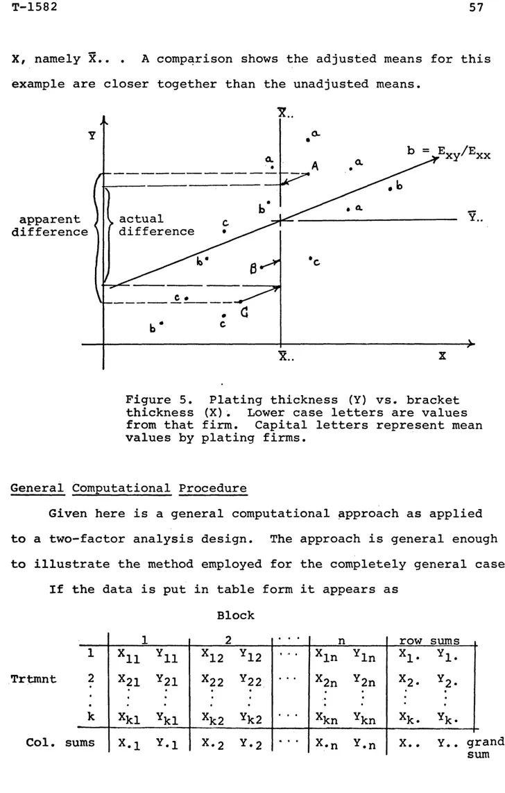
General Computational Procedure... 57
Specific Results... 64
Reduction in Variance (Error Control)... 64
Adjustment of Means... 64
As sumpt ion s ... 65
Tests of Assumptions... 66
Multiple Covariance... ... ... 69
Multiple Regression Model... 69
Adjustment for Regression... 72
Multiple Covariance Model . *... 72
General Example— 2 Factors, 3 Covariates... 73
General Computational Approach... 74
Uses... 79
Direct Applications... 79
Indirect Applications... 83
Estimation of Missing Data... 83
Regression in Multiple Classifications 84 Outlier Points... 84
Regression Adjustment... *... 85
Pooling Data... 87
Individual Yield Estimation... 88
Applications in Special Experimental Design Situations... 88
Pitfalls in Applications... ... ... 89
USE OF THE COMPUTER PROGRAM... 92
Purpose. ... 92 Documentation... 92 Input... 97 Execution... 101 Output... .. ...102 APPENDICES... 109
A. Consequences of Assumptions being Unsatisfied for ANOVA... 110
B. Estimation of ... 114
A C. Decomposition Proof for Total Sum of Squares.... 115
D. Mutually Distinct Partitioning...116
E. Two-factor Decomposition... 117
F. Solution of Normal Equations for Multiple Regression... 118
G. Residual Sum of Squares Deviation... 121
H. Derivation for R ^ ... 122
I. Computer Program Listing... 123
LITERATURE CITED ... 151
ACKNOWLEDGMENTS
I wish to express my thanks to Prof. William Astle, my thesis advisor, for reading and rereading the earlier drafts, for his suggestions contributing to the final form of the thesis, and direction in its completion. Also to Dr. John Kork and Dr. Raymond Mueller, the thesis committee members, I extend my thanks. I also wish to thank Prof. Baer for his assistance in using the computer and especially I wish to
acknowledge Dr. Raymond Mueller for his patience and instruction during my graduate study.
I also gratefully acknowledge the financial aid given by the Colorado School of Mines in the form of teaching assistantships and tuition waivers.
INTRODUCTION
The primary purpose in collecting data is usually to be able to interpret the data as saying something about, or in some way describing, the processes or things being studied. Many diffi culties can arise which make the interpretation of the data dif ficult. One of these difficulties is a lot of variation in the data. Unless this variation can be explained or reduced it is hard for the experimentor to draw conclusions with much precision or definiteness. There are several methods used in attempting to reduce or control variation among the data. Some of these methods a r e :
(i) Exercise control over the homogeneity of the material being tested, and over the experimental environment, thus helping to create uniformity of conditions under which the experiment is performed.
(ii) Group the material and the environment so that (i) holds for the subgroups, i.e., divide the experiment to achieve homogeneity within subgroups.
(iii) Refine the experimental techniques, so that they
are consistent throughout all phases of the experiment and don't contribute to variation in results.
If the experimental techniques are stable and it is not pos sible to subdivide the elements of the experiment into homogeneous subdivisions to control experimental variation, there is a fourth
technique available:
(iv) Measure the variables related to the variable of interest, and use analysis of covariance.
The analysis of covariance is a statistical tool which can be used to identify in a variable of interest, Y say, the amount of variation which is a result of variation in another variable, say X, upon which Y is dependent. Analysis of covariance can then be applied to remove this variation from the variable of interest. The related variates are referred to as concomitant variables.
The presentation of analysis of covariance which follows is on a level which can be understood (hopefully) by a person who has had little background in statistics. A review of regression analysis and analysis of variance, which are vital to analysis of covariance, is presented in the first two chapters to help
introduce notation and make the whole of the presentation as self- contained as possible.
The last section of the chapter on analysis of covariance presents several different applications. Although it is not feas ible to present each of them in computational detail, references for further investigation are given if the reader is interested. The objective is to show the versatility of the technique and the information which is available for what is usually only a small investment of additional computational effort. There are many instances, in fact, where the measurements of what would be the concomitant variable are already known, or are readily obtain able, but because the experimentor is not aware of analysis of covariance, this additional data is not used.
The last chapter shows how to use the computer program which is available, and how to read the output.
LINEAR REGRESSION ANALYSIS
Introduction
In working with statistical problems, many times there is
an association between two or more of the variables being measured, and it would be helpful to establish a relationship, from the data, which would make it possible to estimate, or "predict", one or
more variables in terms of other variables. One of the oldest, and probably one of the most useful, types of relationships is what is called a linear model. Such a model, or relationship, enables the experimentor to use additional, or known, information to help describe the behavior of the variable of primary interest. Such a relationship might make possible a prediction of the amount of sales of a new product from its price, or a student's future grade average from his I.Q. rating or entrance exam score.
Although it would be nice to be able to predict one quan tity exactly in terms of others, it is hardly ever possible, so estimation of an "average" value in terms of others usually has to suffice. /For example, it is not possible to predict the exact number of sales of a product from its price, but it may be possible to estimate the "average" number of expected sales based on infor mation about past performances of like products.
The 19th century English mathematician Francis Galton deve loped the idea of "regression" in his studies of heredity. Speak ing of the "law of universal regression" he said that "each pecul
iarity in a man is shared by his kinsman, but on the average in a less degree." To back this up, he collected data on the heights of fathers and their sons. It was found that although tall fathers tend to have tall sons, the average height of the sons of a group of tall fathers is less than the average height of their fathers. So we say there is a regression, or going back, of sons' heights toward the average height of all men.
In mathematical jargon, we would probably say that the pre dicted variable, say Y, is a function of the variable upon which the prediction was based, call it X , but in statistics Galton's term "regression" is usually used so that the relationship found between Y and X is called the "regression of Y on X ."
The Regression Model
As an example, suppose we were interested in studying the weights of a certain population of men, and the relationship be tween the weights and the heights of these men. To study this the men are subdivided into groups according to height so that the men in any one group are all very nearly the same height, and the relationship between weight and height is examined by looking at the various subdivisions and their weights.
It is obvious that for any particular height there will be a whole range of weights. Not every man that is six feet tall will weigh 18 0 pounds. There will be light ones and heavy ones. This distribution of weights for a particular height has a mean value. In statistical language this would be called the expected value for the weights. This distribution would also have a
var-iance, the variance of weights of all men who have this height. The "regression of weight on height" in this case would be the relationship between the heights and the means of the distribu tions of weights for each of the heights. The regression rela tionship doesn't allow a prediction of a man's weight, given his height, but the average weight of all men who have that height can be predicted.
It can be seen here that the distribution of weights depends on the height chosen, and so weight would be referred to as the dependent variable, and height as the independent variable.
Introducing some common notation, the dependent random var iable, which is usually the variable of interest, is denoted by
Y and the independent variable by X, although any symbols may be used. The mean value for the distribution of Y, called the ex pected value, is denoted by E(Y ) . The expected value of Y given the variable X has taken on the value X, denoted E(Y|x), is cal led the conditional expected value of Y. It could represent the expected value for the weights given the height chosen was X. If we write E(Y|X), this represents a whole set of conditional expected values of Y as X takes on all values in its domain.
In regression analysis, we want to determine what the rela tionship between X and E(y |x) is, so that if we know the indepen dent variable X has taken the value X, it is possible to predict the mean value of the Y for that X, E(Y|X). A first approximation to this relationship, and usually a good approximation, especially over short intervals, is a straight line. This could be written
as
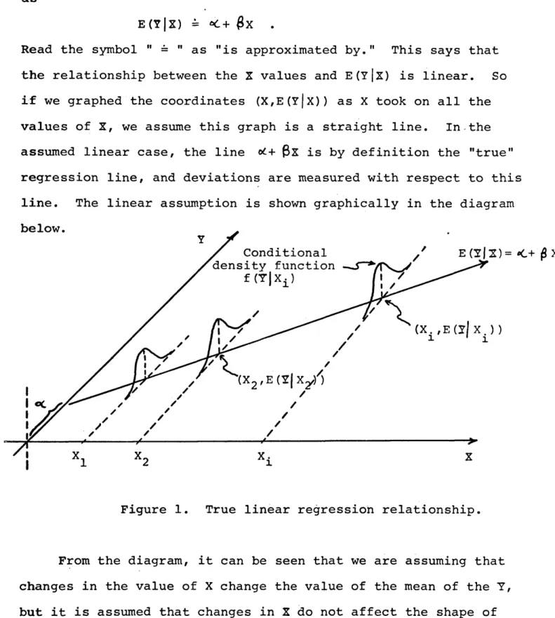
E(Y|X) = *<- + $ x .
Read the symbol " = " as "is approximated by." This says that the relationship between the X values and E(y |x) is linear. So if we graphed the coordinates (X,E(y |x )) as X took on all the values of X, we assume this graph is a straight line. In the assumed linear case, the line od + Px is by definition the "true" regression line, and deviations are measured with respect to this line. The linear assumption is shown graphically in the diagram below.
/ Conditional density function
f (T|X± )
Figure 1. True linear regression relationship.
From the diagram, it can be seen that we are assuming that changes in the value of X change the value of the mean of the Y, but it is assumed that changes in X do not affect the shape of
given later.
It should be understood that in general the straight line is an approximation of the actual relationship between Y and X. Also, because Y is a random variable, in general, observed or measured values of Y will not be equal to the predicted value. That is, the observed values of Y will not all fall on the line E (y |x ) .
The observed value of Y can then be written as y = e(y|x) + e ,
where € represents some error, the amount of Y not accounted for by the regression line of Y on X. This is logical, since for each
X there is a whole population of Y's, of which we have observed one. We would expect, in general, that this one we observed will not always be the mean value, E(Y|X), of the population of Y's for that X. The amount that the observed Y differs from the mean value is represented by £ ;
Since, in the linear case, E(y|x) = o t + @X, we can rewrite this relation as
Y = «C + @ X + £ ,
where Y is a measured or observed value of Y for X taking on the value X.
It is assumed here that the only error involved is in observ ing the Y, that the X is measured without error, so that the error , is entirely included in £ .
The relationship above is for Y dependent on only one var iable, X. The situation may arise where Y is influenced by k fixed variates, X^, X2/ ... / X^. This is covered in chapter 3.
If our data consists of n observations of Y and X, simul taneously, then we have n points, |(X^,Y^), i=l,2,...,nJ , and each observed Y could be modeled
Y i = *•+ P x i + £ i •
It remains now to find out what <>C and (3 are so the regression model is usable.
Determining The Regression Relationship
To be able to use, in the linear case, what we define as the true regression relation,
Y = E(Y|X) + C = c C + $ X + e ,
we have to know the joint probability density function for X and Y to compute the true conditional expectations of Y. Since with fresh data this information is rarely available, the relationship between X and Y has to be estimated from the data on hand. If we have n observations on X and Y, we hope to use these to estimate the expected value of Y for each X value, i.e., E(Y|X^), i=l,...,n.
A
If Y^ is used to denote an estimate (however obtained) of the ex pected value value of Y, given X is X^, E(Y|X^), then each of the observed values, Y^, can be represented by
Yj^ Y^ + e^ , 1=1,2, • . . ,n ?
where Y^ is the estimate of E(y |x^), and e^ is what is called the A
residual, e^ is the amount by which the estimated value, Y^, mis sed the observed Y^. £ ^ is the deviation of the observed value, Y^, from the true regression line, E(y |x), and e^ is the deviation
. A
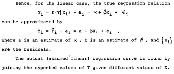
Hence, for the linear case, the true regression relation ya = e(y|x± ) + = ° t + (3xi +
can be approximated by
+ e^ = a + bX^ + e^ ,
where a is an estimate of oC , b is an estimate of ^ , and are the residuals.
The actual (assumed linear) regression curve is found by joining the expected values of Y given different values of X. This relation is compared to the estimated regression line below.
observed value
T=a + b X (estimated)
Figure 2. Comparison of true and estimated regression lines.
For a given observation (Xj^Y^), the true error is given by € i = Y i " E <Y lx i) = Yi - (* + 0 ^ ) (1) and the estimated error, or residual, by
Estimation of Parameters and £
There are many methods for determining values for a and b, the estimates of oC and $ , from the data to obtain a "best" fit of the line to the observed points. No matter how it is done, it seems reasonable to try and make the residuals, r as small as possible. The problem, then, is how to go about making them small. Among possible approaches are:
Method (iii), called the "method of least squares", is one of the easier methods to apply, and under certain assumptions, it provides estimates of < and ^ which are unique, and the best
(linear) unbiased estimators.
Before showing how this method can be applied, some of the assumptions which are made for the linear regression model least squares estimation should be noticed.
Assumptions. The basic assumption, of course, is (i) that the conditional expected value of Y, given X, E(Y|X), is a linear function of X. It is also assumed (ii) that the conditional den sities for Y are uncorrelated for different values of X. This is usually reasonable to assume, and just means that the value Y takes on for one value of X does not affect the value Y takes (i) Minimize the sum of the absolute values of the e^,
i.e., minimize 21 leil •
(ii) Minimize the greatest of the absolute residuals, i.e., minimize
(iii) Minimize the sum of the squares of the residuals i.e., minimize .
on for another value of X. Thirdly, we assume (iii) that the X values are measured without error, so that all the error in the model is represented in the error term, 6 . We also assume that the conditional variances of the Y populations are independent of X. That is, the variance of Y is the same no matter what val ue X takes on. These assumptions are enough to be able to apply the method of least squares with assurance that the estimates of
©c and ^ are "unbiased" (see [22], pg.147) and have the smallest variance of any estimators. If however, it is desired to make the usual tests of significance (such as the t- and F-tests) of our estimates (to see how sure we are about how good we think the estimates are), it must also be assumed that Y is distributed normally (or that X and Y, jointly, are distributed as a bivar- iate normal). This means that the Y's are not just uncorrelated, but independent, and that we can say that the error terms,
are independently and normally distributed with mean zero (see equation (1)) and a common variance, <jr .
Least Squares Estimation. Let us consider the problem of estimating the best linear approximation of the relationship be tween Y and a single fixed variable, X, using the method of least squares, so that observed values of Y are given by
Y = cC + (3x + £ = a + bX + e
where oL and p are unknown parameters and a and b are their res pective estimates, €, is the true error, and e the residual
A A
(e = y - Y, where Y = a + b X ) . We now assume -that a sample of n X's are selected (without error) and corresponding Y's are meas ured. Using the method of least squares, we form what is called
the error sum of squares, usually represented by SSE, SSE = £ ei2 = ^.(Yi - (a+bXi))2
= £ < Y i - ^ - b X ^ 2 .
We want to determine a and b so as to minimize SSE. This can be done by taking partial derivatives of SSE with respect to a and b, setting the two resulting equations equal to zero, and solving this system of equations for a and b.
Taking derivatives, first with respect to a, then with res pect to b, equating the derivatives to zero, and rearranging them into what are called the "normal"* equations, we obtairi
£ y . = na + b £ x .
Zx.Y, = a £ x . + b'£Xj 2 , for i=l,2, . .. ,n. i 1 i 1 i 1
We then solve these two equations simultaneously for a and b. An example follows.
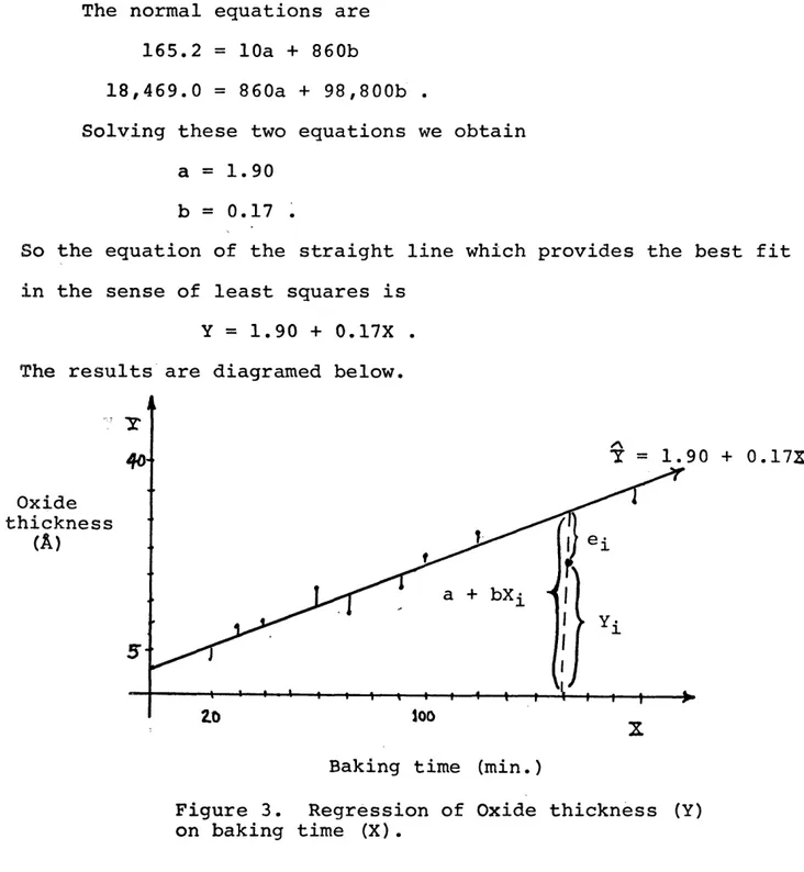
Suppose we are given the set of paired data below (data from Miller and Freund [32]), where the X's represent baking time, in minutes, of a mineral specimen, and the Y's are the oxide thick nesses on the specimens in Angstrom units resulting from the bak ing. We examine the thicknesses resulting from 10 different bak ing times.
Time 20 30 40 60 70 90 100 120 150 180
Thickness 3.5 7.4 7.1 15.6 11.1 14.9 23.5 27.1 22.1 32.9
7 ^ = 860 £ x ^ = 98,860 = 165.2 £ xiYi = 18,469.0
The normal equations are 165.2 = 10a + 860b
18,469.0 = 860a + 98,800b .
Solving these two equations we obtain a = 1.90
b = 0.17 .
So the equation of the straight line which provides the best fit in the sense of least squares is
Y = 1.90 + 0.17X . The results are diagramed below.
Y = 1.90 + 0.17X Oxide thickness
(A)
5* looBaking time (min.)
Figure 3. Regression of Oxide thickness (Y) on baking time (X).
Residual Sum of Squares Form
There is a second approach we might use in solving the normal equations for a and b, giving a different form for the regression model and resulting sometimes in easier calculations.
Taking the partial derivative of the error sum of squares with respect to a, equating it to zero, and solving for a, we have
d SSE = 0 =£> ]FY ■ = na + b '
Z
x i 7d a h ence,
a = Z.Yi/n “ (b-2.Xi )/n = Y - bX . > We know this solution for a results in a minimum sum of squares, rather than a maximum, since no finite maximum exists.
If we insert this value for a into the original SSE equation, we get that
SSE = 7(Y. - a - bX.)2
1 1 1
= 7 [(Yi - Y) - b(Xi - X)] 2 = 7 (yi - bX i >2
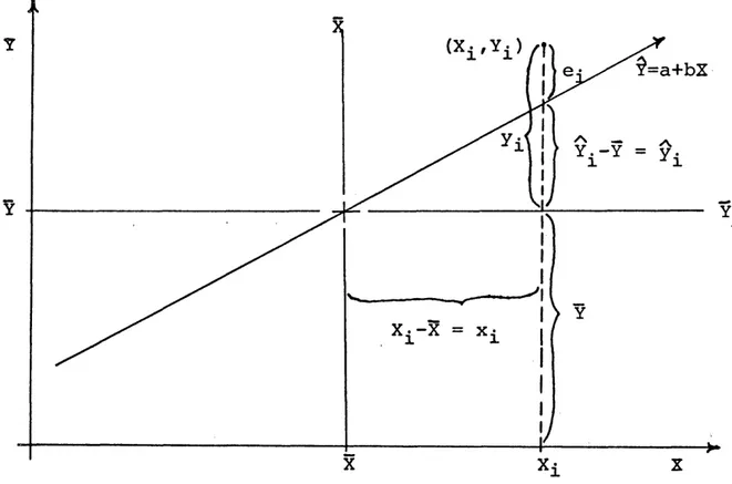
where y^ = Y^ - Y and x^ = X^ - 5C. Using this value for a we could rewrite the regression model as
Y = a + bX = Y + bx
Taking the partial derivative of this new form with respect to b, equating that to zero, and solving, we obtain
^ [Z.(Y - bxjJ2] I x i.Yi
5 b - 0 b - £ x i 2 (2)
where =
Z(X±-X)
(Yr T) = - [{£ X ± ) <Zx
±2
= Z(Xi.-X) (Xi-X) = Z x i2 - (Zx i2)/n
We can use this new information to find the amount of the
2
total error sum of squares ( Z y ^ ) which is actually due to var iation among the X, causing variation in Y by means of the depen dency of Y on X, which might not otherwise have been there.
Using the new model Yi = y i + ei
= Y + bx^ + e^ and rearranging to solve for e^,
= (Yi -.7) - bx^ = Yi - bx± .
Using this deviation form to reconsider the residual sum of squares we obtain
= Z(Yi - bxi)2
= Z y ± 2 - 2b-£xiyi + b 2'£.xi2 .
Substituting for b the least squares estimate obtained above in equation (2), we have that
T 2 _ 2 . <- 2
= L y± - 2 ^ x ,2 "L * iYi + Z x i (L x iYi)2
=
Z
y±
Zx.
(3)The Regression Adjustment in the Error Sum of Squares
Looking at this new result, equation (3), for the residual sum of squares we see we are reducing the original error sum of squares, prior to regression, which is
^ 2 c 2
by the amount
£ (y . - y)2 = 2vi'
( Z x i y .)
Z x i
This is the amount of the error sum of squares that we can "explain" as variation among the Y values due to variation in the X values,
transferred through the dependence of Y on X.
The new adjusted sum of error squares can be viewed in a different way which may make clearer what this sum represents.
_ 2
2,(Y^-Y) gives an estimate of the variation among the var iable of interest, Y, before we use any information concerning the dependence of Y on a concomitant variable X. Using this in formation as we did above, we obtained the new resultant estimate of variation. Rearranging equation (3), we get that
Z(Yi-Y)2 = Z Y i 2 = ( 2 * ^ ) 2
Zx.
T residual + sum of squares The residual sum of squares is found by subtraction, so thatResidual S.S. = £ ej.2 = ~ (£ x iYi)2
2 Z
xi
— 2
The total sum of squares of Y, £ Yi r has been partitioned
1
into two parts:
(i) A sum of squares attributable to variation among the X's, said to be "attributable to regression."
(ii) An unexplained portion, the residual sum of squares. It may be of some assistance to show graphically what has
been done. This is done in the diagram on the next page (Figure 4) From the diagram it can be seen that the two forms of the regres sion model are equivalent. That is, that
and
Y^ = a + bX£ + e^
Yi bx^ + e^ are equivalent.
Y
$=a+bX
-Y
Figure 4. Deviation form of the regression model.
As a further explanatory note, we may notice something more from Figure 4. We know that the reduction in the sum of squares of the error term e is given by
< Z x iyi>2/ < Z x i2 ) = b - Z ^ V i • Reducing this, we obtain
b '2x iYi = [< Z x iy i )2/ ( £ x i2 )2 ] • ( £ x i2 ) = b2 Z x i 2 = I b 2x . 2 c A 2
= Z yA
=Z
(?i-Y)2.
So the sum of squares attributable to regression turns out to be
A
the sum of squares of the n deviations of the estimate, Y, from its mean Y. What we have actually done by subtracting this amount
out is to measure the variation among the Y's as if they had all been measured for a standard value of X, namely X. Since it would be tedious to calculate the sum of squared deviations of estimates from their mean, we use the shorcut form given in equation (3).
As a final note, we can now estimate the variance of the ran dom variable Y which is not attributable to variation in X. The residual sum of squares, the unexplained part of the variation in the Y's, divided by (n-2), its degrees of freedom, gives us the residual mean square and is an (unbiased) estimate of the var iance of Y. It is usually denoted by s a n d is defined by
s? = SSE (adjusted) = £ y . 2 " <
I
x iYi.) V Z x i2y x 1 —
n - 2
- 2>i2
■
—
H
U
■
•
n-2
It measures the amount of variation in Y not associated with, ex plained by or dependent upon changing values of the fixed variate X.
ANALYSIS OF VARIANCE
Introduction
First introduced by Sir R. A. Fisher of England in the early 1930's, the term "analysis of variance" has come to rep resent the use of a number of statistical techniques whereby the experimentor is able to examine the variability occuring in a group of data, and separate the variance ascribable to one group of causes from the variance due to other groups of causes. By
separating, and identifying, different sources of variation in the data and the amount of variation each contributes, the ex perimentor is aided in making judgements about the populations
from which the data has been drawn.
One important use of some of these techniques is as an aid in determining if the differences between means of different sam ples can be attributed to chance variation or if these differences
indicate actual differences between the true means of the corres ponding populations from which the samples were taken. Therefore, we want to analyze the variability that occurs in the entire group of data and determine its sources.
To illustrate the basic idea with an example, suppose a man can drive from his home to work along any one of three different routes, and he would like to know which of the three routes
is the fastest. He records the time it takes him along each route on five different days, shown below in minutes.
Route 1 s 22 26 25 25 31
Route 2: 25 27 28 26 29
Route 3: 26 28 27 30 30
The means of these three samples are 25.8, 27.0, and 28.2. Since the size of the samples is so small, we would like to know whether the differences among these means is because the routes really do, on the average, take different amounts of time to travel, or if the differences are just due to chance variations along the routes during the five days on each route.
To treat this kind of problem in general, suppose we have k independent samples (random) of size n * , each from one of k populations, and let X ^ represent the jth observation from the ith population. We can express each of the observations, as well as the samples, in table form as shown below.
Sample Means Sample Is ^11 ^12 * * ” ^li * * * ^ln ^1» Sample 2s ^21 ^22 * * ' ^2i " * * ^2n ^ 2 # Sample ks X^2 • • • ^kn ^k grand mean X . . Table 1.
♦Although computationally easier, it is not a requirement that the samples be of equal size. If the samples are of differ ent sizes, we calculate the overall mean by weighting sample means according to the size of the sample.
These sample groups are often referred to as "treatments", owing to the origin of this method in the field of agriculture.
The dot as a subscript means that the variable has been sum med for the subscript which has been replaced by the dot. For example,
X x . = Z
-L
x h-«-j
/ and in generalX. i - = Z x -i-i ^ 13
The means are calculated as x± . = ( Z x ..)/n ,
1- ) 13
X . . = ( 7 Z X±i ) /nk
l ‘ l J -t 3
Each of the k samples comes from a population with a true mean, m^ 0 say, which has been estimated by X ^ # . We are inter ested in learning something about the relationship between the means of the populations. More specifically, we are concerned with testing the fact of whether the means of the populations are equal or not. Mathematically, we want to test the hypothesis that all k populations have the same (true) mean. Symbolically,
H0 ; m^ = m2 = ••• = m^ = m ..
is the hypothesis that is to be tested.
Each of the observations can be expressed now as
Xij = m^ 9 + 6 ij , i=l,2,...,k 7 j= l,2,...,n, where the ^ r e p r e s e n t (random) "error" deviations of the ob
servations, X ^j, from their respective sample means. This model can be further generalized to
Xj • m.. + ^ j • t 1 1,2,...,k 7 3 l,2,...,n.
where is the deviation of the ith sample mean, m ^ # , from the grand overall mean, and £ ^ again is the deviation of the observation from its sample mean.
The hypothesis of equal population means which is to be tested could also be expressed as
Hq : = 0 for every i. The alternative to this hypothesis is
7^ 0 for some i,
or in other words, at least one of the population means differs from the grand mean.
Before continuing to see how this hypothesis could be tested, it is important to consider the assumptions underlying the analysis or variance model and the practical importance of each.
Classes of Analysis of Variance Problems
Two distinct classes of problems are solvable by analysis of variance (ANOVA). Although the calculus of the analysis in either case is the same, there are two major ways to interpret the results. If we use the analysis as a "fixed-effects model", we mean that we are comparing these k sample means and will draw conclusions about only the k population means involved in the analysis. If, as a result of the analysis, it is decided that there is a difference among the k means, we interpret this as meaning that at least one of the k population means differs from
the others. In other words, that there is a difference of means among these k fixed treatments. On the other hand, if we con sider this as a "random-effects model", we interpret a difference
among sample means as not indicating a difference among k fixed treatments only, but rather indicative of a difference among all possible treatments which could have been examined (e.g., all possible routes which led to work in the first example of com paring three particular routes). That is, we take this differ ence as an inference of fixed differences among individual treat ments of a particular generic type.
Since the questions to be answered by the data are differ ent in each of these two cases, the models are interpreted dif ferently. Although the algebra involved is the same, the assump tions underlying each differ somewhat.
Assumptions
The algebraic procedure employed to construct the analysis of variance results is true, no matter what the numbers involved represent. Hence, it holds for both fixed- and random-effects models.
Consider k*n numbers arranged in a matrix of k rows and n columns, and X - • denotes the number occuring in the ith row and
J
the jth column of this array. If we border the array with row means we obtain a configuration like the one below.
1 2 • j . . . n row means 1 X 11 X 12 •• x i r • • x ln x i. 2 X 21 X22 • • x ?j • • • • x 2n • X 2-• i • » X f1 X i2 • • x f j . . . xin *!• k xkl Xk2 ' • • xkj • • • xkn X. .
Fixed-effects Model
When the formulas and procedures of analysis of variance are used to summarize certain properties of the data on hand and nothing more, no assumptions are needed since it is just an em ployment of algebra calculating and comparing means. However, if from the data on hand in the samples inferences about pro perties of the "populations" from which the data was drawn are to be made, then certain assumptions about the populations, and about how the samples were obtained, must be made if the inferen ces are to be valid.
No statistical inferences can be made from the numbers X^j unless they are assumed to be observations of random variables of some sort. So that must be the first assumption, that (1) the numbers X^j are (observed values of) random variables that are distributed about mean values m^j , (i=l,2,...,k;j=l,2,...,n), that are fixed constants.
It is possible to arrange the parameters m^j into a table form like Table 2 for the X ^ j , bordered by the row means, m ^ . It is apparent now that the value X^2 " x 52 9ives an unbiased estimate of m ^ ~ m 52 • so now we can ^raw inferences from the data concerning the means of the populations from which the data was drawn. In fact, assumption 1 allows that the unbiased esti mate of any linear combination of the m^j is provided by the same combination of the X ...
13
If the true mean values m^j in such a table are additive functions of the row means and grand mean, that is, if
m ij = ^m ij - m i •) + m . .
= m . . + (m^# - m..) + (mij - m i.) (D then the inferences that can be drawn from the data are much more general. If equation (1) is satisfied by the model, that
is, if equation (1) represents the relationship among the data, then the difference between any two row means, m ^ # ” m 2. ^or ex" ample, which is estimated by X ^ # - t is a comprehensive esti mate of the difference between the two row means. However, if equation (1) did not hold, then X ^ # ” ^2. woul^ estimate the dif ference between the two row means for this configuration only, with the column-wise data (j=l,2,.«.,n) in the particular order they are in and the rows in their present order. This is because if the additivity (equation (1)) does not hold, "interaction" effects between certain rows and columns are present, adding a hidden effect not represented in observation/row-mean deviation or in row-mean/grand-mean deviation.
Therefore, in order to be able to draw general inferences concerning sample, or row, population means, regardless of the par ticular order they happen to be in for the experiment, we assume that (2) the parameters m^j (and hence estimates from the j ) are related to the means m-^. and m.. as in equation (1), namely,
m ij = m * • + (m i. ” m . .) + (m^j - for i=l,2,...,k and j=l,2,...,n.
With assumptions 1 and 2 satisfied, the estimate of the dif ference between any two row means from the observations is an un biased estimate of the general average difference between the two row populations concerned, regardless of column order or row order because we assume there are no non-additive effects, and the
addi-tive effects can be summed in any order.
If we want to be able to say something about the variance of the X ^ j , and from that the variance of the population means and linear combinations of them, to get some idea of the preci sion of our estimates, we must go further with the assumptions.
In general, it is not possible to derive unbiased estimates of the variances of the ^ , nor linear combinations of them either, using regular analysis of variance techniques unless assumptions 1, 2, and 3 given below, are satisfied.
We assume that (3) the random variables all have a common variance, , and that they are mutually uncorrelated.
Usually uncorrelatedness is a very reasonable assumption. This means that the amount of error in one observation does not affect the amount of error in another observation. A special approach, called randomization, is used to help ensure this un correlatedness. • The experimentor selects experimental units at random and measures them separately. Hence, the error for any one sample is independent of that for any other sample.
Cochran and Cox [ 6 ] (pg. 8) make the following remark con cerning randomization: "Randomization is somewhat analogous to insurance, in that it is a precaution against disturbances that may or may not occur and that may or may not be serious if they do occur. It is generally advisable to take the trouble to ran domize even when it is not expected that there will be any serious bias from failure to randomize.
compu-tationally it is desirable that the errors have the same variance from one population to another, and aren't effected by different "treatments" (row differences). This is probably one of the more critical assumptions, and one of the hardest to be sure of. Sev eral tests for homogeneity of variance exist. One of the more common is Bartlett's test. This test is given in some detail in Ostle [34] .
When these three assumptions all are satisfied, an unbiased estimate of the difference between two row means, and the variance, can be calculated. If assumption 3 does not hold, then*the covar iances between the X^j are not zero, and the estimates of the var iances of combinations of the data become complex weighted ave rages of variances and covariances.
We now have a means by which the variances of row means, and other combinations of data may be identified and estimated, and so we have a method for judging whether real differences ex ist between population (row) means, which is the objective of the analysis of variance. However, we now have a means by which we can tell the accuracy, or significance, of our judging, and exactly how "sure" we are that differences among true row populations do exist. To be able to do this, i.e., assign some kind of quanti tative probability level reflecting the "sureness" or signifi cance of the variance estimates, we must know something of the joint distribution of the X ^ ^ . Fortunately, "normality", in addi tion to assumptions one through three, allows us to make exact tests of significance. Therefore, we assume (4) that the X . . are
jointly distributed in a multivariate normal distribution.
This assumption allows us to use such tests of significance as the t test and the F test, as will be shown later. This assump tion is probably least likely to be completely true? however,
much of analysis of variance can be used without using this as sumption. The parts requiring normality have been shown to be fairly robust, that is, a fair amount of departure from normal ity can be tolerated without the accuracy being greatly affected.
Note that with assumption 4 made, assumption 1 is nearly covered, serving mainly now to define the means, ^ . Also, the fact that the X^j are assumed uncorrelated in assumption 3 taken together with the assumption that they are normally distributed in assumption 4 implies that the X^j are mutually independent. Further results of these four assumptions will be shown as we con tinue with the analysis of variance model.
For the fixed-effects model, the basic assumptions, in sum mary , a r e :
(1) The observations X are (observed values of) random ij
variables distributed about true means (expected values) m i j ' (i=l/2,...,k? j=l,2,...,n) , which are fixed con
stants.
(2) Additivity. That is, if we define the true grand mean as
/ < = IZroij/nk
' 1 ) J
and define a "row effect" as
/*-then the parameters m^j can be expressed as - / * + ^ *
2 (3) The random variables X^j have a common variance o'
(usually unknown).
(4) The X^j are independently distributed in a multivariate normal distribution.
These assumptions are shown in construction of the model in the following way: If we assume that an observation may be rep resented as
X ± j = y U . + ^ ^ 7 1 — 1 ,2,...,k , j=l,2 ,...,n , where
Z. °£. = 0 ( yU is the grand mean) ,
1 1
and the error terms S .. are normally distributed with mean zero and a common variance o'2 , then we can validly apply analysis of variance techniques.
Random-effects Model
In considering the random-effects model, although algebraicly it is identical to the fixed-effects model, since different in ferences are made from the results slightly different assumptions are made.
We assume (1) that the X . . are, again, (observed values of) 13
random variables distributed about a common mean value / where JL{.
(defined as before) is a fixed constant.
component random variables, such that
where oC . and €. . are both random variables.
1 13
(3) The random variables and are distributed with
2 2
zero means, and variances and o' , respectively.
(4) That the random variables 0 and are independently and normally distributed.
Results of Unsatisfied Assumptions
For a brief discussion of the consequences when certain of the assumptions are not satisfied, refer to Appendix A. For a more thorough discussion, refer to an article by Cochran [5], and to Cochran and Cox [6].
Some Terminology
It will be useful to learn some conventional terminology which may help in describing the set-up of an experiment more precisely. The basic concept is that of a factor, which cata- gorizes some property of the data according to which it — the data — will be classified. For example, in an agricultural ex periment the factor may be fertilizer, to determine the effects it has on crop yield. In measuring the yield data, it would be classified according to the fertilizer used on that plot of ground. If the plots were in different parts of the country, then there would be (at least) two factors, the fertilizer and the climate, that we should consider. The term level refers to particular properties defining subgroups of the factor groups. Thus, the levels of the factor fertilizer would be the different
fertili-zers used. The levels for the climate factor might be set up as the regions in which the plots were located, e.g., Pacific North west, Southwest, etc., or they might be set up in some other man ner, e.g., dry, moderately dry, humid, etc.
We can describe the structure of an experiment, or the exper imental design, by describing the factors and the way in which the levels of the different factors are combined. In the example in which the driver compared driving times taking three different routes to work, there was only one factor we were considering, the route taken. The levels were the three different routes, route 1, route 2, route 3. Hence, we had a one-factor experiment with three levels.
Preparation
Setting Up the Experiment
First, a realistic model must be set up so that the obser vations, j , whatever they represent, can be obtained and are
in a form that can be used in the analysis of variance techniques. (For example, in an experiment where results are obtained as shades of a certain color, these results would have to be quantified be fore they could be used.) The detail of how the experiment is then going to be run, once the model is decided on, should be outlined.
(1) The objectives of the experiment should be clearly de fined. For instance, if the experiment is a preliminary one to
determine what future experiments should be like, or if it is to get answers to immediate questions. Is it mainly to get "ball park" estimates or is the experimentor mainly interested in tests
of significance (accuracy)? Over what range of conditions are the results to be extended?
(2) The experiment should be described in detail. The dif ferent factors to be considered, the levels the experimentor wants to test for each factor, the size of the experiment, and the mater ial necessary to complete the experiment.
(3) An outline of the analysis to be done would be helpful to have as a guide before the experiment is started so that the data necessary to the analysis is obtained.
Running the Experiment
The experimental techniques should be refined as much as possible.
(1) There should be a uniform method of applying different treatments to the experimental units.
(2) Control over external influences should be exercised as much as possible so that every treatment operates under as nearly the same conditions as possible.
(3) Unbiased methods of measuring results should be devised so that the results are as objective as possible and can be com pared with results from other experiments. As an example, it is difficult to measure objectively educational progress, social
standing, or socio-economic levels since these are by nature subjective judgements.
(4) If possible, checks should be set up to avoid making, and admitting to analysis, gross errors in experimental measure ment, since one or two such errors could bias the entire results.
Further information along this line is included in many texts including Cochran and Cox [«J, Johnson and Leone Snedecor [3 Ostle [34], or other standard statistics texts.
Analysis of Variance
We will consider our models, and examples, as being fixed- effects models. Some authors vary notation to indicate which model they are working with. Notation here is fairly consistent with that used in Probability and Statistics for Engineers by Miller and Freund [32].
One-way Classification
The objective, once again, is to determine if the means of the populations from which the different samples have been taken are equal. We approach this by analyzing the variance among the sample, or treatment, means and attempting to judge whether the amount of variance is due only to chance variation, in selecting a sample from the population, or indicative of actual differences among means of the populations. Recall that our null hypothesis, HQ , was that the true (row, or treatment) population means were equal,
Hq : - ^ 2 “ = •** “ /^k = (grand mean). To test the hypothesis of equal means, we first need to find the total variability of the combined data. This quantity is usually referred to as the "total sum of squares", and is denoted
where X,. is the overall mean of all observations,
If Hq is true, the SST is totally due to chance variation. If HQ is not true, then there is a contribution to variation due to differences among the means of the k populations.
To test this hypothesis that the k population means are equal
•y
we compare two estimates of the variance
o '
, the variance of the observations ^ . One estimate is based on the variation between the sample (or treatment) means, and one is based on the variation within the samples.If the hypothesis is true that the population means are equal then these are estimates of the same value, O * ^ , and should be approximately the same. However, if the hypothesis is not true and in fact there is a difference between population means, this difference will "inflate" the estimate based on variation among sample means, making it larger than the estimate based only on variation within the samples. Hence, if the null hypothesis is false, that is, if all population means are not equal, we would
2
expect the "between sample" estimate, s B say, to exceed the 2
"within sample" estimate, s Forming a ratio of these two
values, we reject the hypothesis, or say there is evidence to in-2 0
dicate the means are not all equal, if the ratio s ^/s w "to° large", i.e., if the between sample estimate is larger than the within sample estimate by enough to indicate a difference of means among the populations.
approaching this problem, let us look at the two variance
esti-2 ?
mates, s B and s*w .
Since, by assumption, each sample comes from a population having variance this variance can be estimated by any one of the sample variances (i=l,2,...,k)
s2Wi = Z(Xij - XijVtn-l)
and, hence, this variance is also estimated by the mean of all these k estimations,
S2W = Z s 2Wi/ k = £F(Xi:j - Xi.)2/k(n-l) .
The variance of the sample means is given by s2^ = Z ( X ± . - X..)2/(k-l)
and if the null hypothesis is true and there is no difference among population means and this variation among sample means is due to chance variation, it estimates O'^/n. (See Appendix B ) . Thus, an estimate of O' based on variation among the sample means is given by
s2b = n-s2^ = n* - X..)2/(k-l)
It can be shown that we now have two independent estimates 2
of the variance
o'
.
The next fact is what allows analysis of variance to work. The two estimates of the variance shown above can be obtained
(except for the divisors (k-1) and k(n-l)) by "breaking up" the total variance of the combined data into two parts. The total variance for the combined data is estimated by
s2t =ZL(*ij - x. .)2/(nk-l) . ^ J
is shown in the theorem below.
SST = ZE(Xij - 5..)2 = Z K X i j - Xi.)2 + n £(Xi. - x..)2 where is the mean of the sample from the ith population, as defined before. (Proof of theorem in Appendix C ) .
What is remarkable is that this decomposition means that the total sum of squares is broken into component sums of squares which are, themselves, squares of, or sums of squares of, linear combinations of the observations, X .., that sum mutually distinct
i
properties of the data, so that one sum is independent of the other. (See Appendix D ) .
Referring to the decomposition above, we see by inspection the first term on the right gives the variation due to differ
ences of observations from their sample means, i.e., within sample variation. This is usually referred to as "within" variation, or error sum of squares, SSE. The term "error" expresses the idea that the quantity estimates random, or chance, error varia tion. The second term on the right gives the variation among
sample, or treatment, means. This is referred to as the "between" variation, or the treatment sum of squares, SS (Tr).
Thus, we have partitioned the total variability of the com bined data into two components: The first, SSE, measures chance variation within samples; regardless of whether the null hypoth esis is true or not, it only measures variation due to chance,
o
and is an unbiased estimator of < f . The second, SS(Tr), also measures chance variation when the hypothesis is true, but it
is affected by the added variation among the population means when the null hypothesis is false.
9 o
In the variance estimators s B and s t h e divisors, (k-1) and k(n-l), are called degrees of freedom. They represent here the number of independent observations of the data, ^ . It can be shown (see Hoog and Craig [27] or Anderson and Bancroft [1] or Larson [3l] ) that the ratios (SSE/deg. of freedon) and
(SS(Tr)/deg. of freedom) are independent, and both have
(Chi-square) distributions. It is this fact that allows us to make tests of significance. Therefore,
[_______ SS(Tr) | f sS(Tr) ] Ltrt. deg. of free.j = [ k-1
J
r________ s s e_______ i[error deg. of freej
SSE
F(k-1,k (n-1)) k (n*
where F is the Snedecor F distribution, with k-1 and k(n-l) degrees of freedom as the two parameters, and where "/%/■" means
"is distributed as." This is true because the ratio of two in- * 2
dependent x. distributions has an F distribution (see references given above). We can now test this ratio of variance estimates to see if it is "too large" by comparing it to a tabled value of the F distribution, to see if it is large enough to indicate a difference of population means.
An analysis of variance table is shown below for a one-factor experiment. Source of variation degrees of freedom sums of squares mean squares F values treatments k-1 SS (Tr) MS (Tr)=s s (Tr) k-1 MS(Tr)
error k (n-1) SSE MSE=SSE = (V2
k (n-1) MSE
Total nk-1 SST
a 2 2