Topology optimization of load-carrying
structures using three different types
of finite elements
S H O A I B A H M E D
Master of Science Thesis
Stockholm, Sweden
2013Topology optimization of load-carrying
structures using three different types
of finite elements
S H O A I B A H M E D
Master’s Thesis in Optimization and Systems Theory (30 ECTS credits) Master Programme in Mathematics (120 credits) Royal Institute of Technology year 2013
Supervisor at KTH was Krister Svanberg Examiner was Krister Svanberg
TRITA-MAT-E 2013:35 ISRN-KTH/MAT/E--13/35--SE
Royal Institute of Technology
School of Engineering Sciences
KTH SCI SE-100 44 Stockholm, Sweden URL: www.kth.se/sci
Abstract
This thesis deals with topology optimization of load-carrying structures, in particular compliance minimization subject to a constraint on the to-tal amount of material to be used.
The main purpose of the work was to compare the following three types of finite elements for the above topology optimization problems: Four node square elements with bilinear shape functions, nine node square elements with quadratic shape functions, and six node hexago-nal elements with Wachspress shape functions.
The SIMP approach (Solid Isotropic Material with Penalization) was used to model the topology optimization problem for different load and support conditions, and the method of moving asymptotes (MMA) was used to solve the formulated optimization problems.
On the considered test problems, it turned out that the results ob-tained by using six node hexagonal elements were in general better than the corresponding results using nine node square elements which in turn were better than the results using four node square elements. The price
Acknowledgment
All prays be to Almighty ALLAH, the most gracious, compassionate and ever merciful WHO has given me knowledge, power and strength to accomplish this task.
I am extremely thankful to my Supervisor, Krister Svanberg under whose patronage, supervision and guidance; I carried out my research work successfully and achieved the goal. His diversified experience, in-depth knowledge and command on the subject benefited me a lot. It was a great opportunity for me to do Master thesis under his able guid-ance and supervision. I will never forget his generous and affectionate help.
Last but not the least, I pay my sincere thanks to my parents whose prayers continually shielded me in all of my life. They always supported me particularly, in a difficult time and encouraged me to move forward. I am also thankful to my brothers and sisters, specially my eldest sister and younger brother for their affection, assistance and prayers.
For further information regarding the contents of this technical re-port, please contact the author: shoaibah@kth.se; shoaib.ciit@gmail.com or the Department of Optimization and Systems Theory, KTH, Stock-holm, Sweden.
Contents
List of Figures List of Tables
1 Introduction 1
1.1 Topology optimization . . . 2
1.2 Finite element method . . . 4
2 Topology optimization problem for compliance minimization 7 2.1 Introduction . . . 7
2.2 Topology optimization model . . . 7
2.3 Optimality criteria . . . 8
2.4 Mesh-independency filter . . . 9
2.5 Method of moving asymptotes . . . 10
2.6 Topology optimization problems . . . 11
2.6.1 Half MBB beam . . . 12
2.6.2 Short cantilever beam . . . 13
2.6.3 Cantilever beam with a fixed hole . . . 14
2.7 Continuation procedure . . . 15
2.8 Results and Discussion . . . 15
2.8.1 MBB beam . . . 15
2.8.2 Short cantilever beam . . . 15
2.8.3 Cantilever beam with a fixed hole . . . 17
3 Comparison of SIMP model and alternative model 19 3.1 Introduction . . . 19
CONTENTS
3.4 Results and Discussion . . . 21
3.4.1 MBB beam . . . 21
3.4.2 Short cantilever beam . . . 22
3.4.3 Cantilever beam with a fixed hole . . . 22
4 Four node square elements, nine node square elements and six node hexagonal elements 25 4.1 Introduction . . . 25
4.2 Finite elements used . . . 25
4.3 Four node square element . . . 26
4.4 Nine node square element . . . 26
4.5 Six node hexagonal element . . . 27
4.6 Results and Discussion . . . 28
4.6.1 40% Volume . . . 31
4.6.2 50% Volume . . . 36
4.7 Another load condition . . . 42
4.7.1 40% Volume - 80×80 . . . 42
4.7.2 50% Volume - 80×80 . . . 46
5 Conclusion and future work 49 5.1 Conclusion . . . 49
5.2 Recommendations for future work . . . 50
A Finite element method procedure 51 A.1 Domain discretization . . . 51
A.2 Displacement interpolation: . . . 51
A.2.1 Local and Global coordinates . . . 52
A.3 Construction of shape function: . . . 52
A.3.1 Properties of shape function . . . 53
A.4 Formation of FE equations in local coordinate system . . . 54
B Shape functions 55 B.1 Four node square element . . . 55
B.2 Nine node square element . . . 56
B.3 Six node hexagonal elements . . . 56
C Gauss integration 57 C.1 Four node element and nine node element . . . 57
C.2 Six node element . . . 58
D Hexagonal element 61
List of Figures
2.1 Topology optimization problems . . . 12
2.2 Half MBB beam solved by OC on left and MMA on right . . . 13
2.3 Short cantilever beam solved by OC on left and MMA on right . . . 13
2.4 Cantilever beam with a fixed hole solved by OC on left and MMA on right 14 2.5 Half MBB beam solved by continuation procedure with MMA . . . 16
2.6 Short cantilever beam solved by continuation procedure with MMA . . 16
2.7 Cantilever beam with a fixed hole solved by continuation procedure with MMA . . . 17
3.1 Half MBB beam solved with alternate model . . . 23
3.2 Short cantilever beam solved with alternate model . . . 23
3.3 Cantilever beam with a fixed hole solved with alternate model . . . 23
4.1 The finite element four node in local coordinates (ξ, η) . . . . 27
4.2 The finite element nine node in local coordinates (ξ, η) . . . . 28
4.3 Square element mesh can display one node-connection while hexagonal mesh shows two node-connection . . . 29
4.4 The square element has two edges-based-symmetry lines whereas hexag-onal element has three edge-based symmetry lines . . . 29
4.5 Design domain, loads and support for square element (a) and hexagonal element (b) . . . 30
4.6 Four node square elements without filter; Volume 40%, N = 60 × 60 . . 32
4.7 Four node square elements with filter; Volume 40%, N = 60 × 60 . . . . 32
4.8 Nine node square elements; Volume 40%, N = 60 × 60 . . . 33
4.9 Six node hexagonal elements; Volume 40%, N = 60 × 60 . . . 33
List of Figures
4.12 Nine node square element; Volume 40%, N = 80 × 80 . . . 35 4.13 Six node hexagonal element; Volume 40%,N = 80 × 80 . . . 36 4.14 Four node square elements without filter; Volume 50%, N = 60 × 60 . . 37 4.15 Four node square elements with filter; Volume 50%, N = 60 × 60 . . . . 37 4.16 Nine node square elements; Volume 50%, N = 60 × 60 . . . 38 4.17 Six node hexagonal elements; Volume 50%, N = 60 × 60 . . . 38 4.18 Four node square elements without filter; Volume 50%, N = 80 × 80 . . 39 4.19 Four node square elements with filter; Volume 50%, N = 80 × 80 . . . . 40 4.20 Nine node square elements; Volume 50%, N = 80 × 80 . . . 40 4.21 Six node hexagonal elements; Volume 50%, N = 80 × 80 . . . 41 4.22 Four node square elements without filter; Volume 40%, N = 80 × 80 . . 43 4.23 Four node square elements with filter; Volume 40%, N = 80 × 80 . . . . 44 4.24 Nine node square elements; Volume 40%, N = 80 × 80 . . . 44 4.25 Six node hexagonal elements; Volume 40%, N = 80 × 80 . . . 45 4.26 Four node square elements without filter; Volume 50%, N = 80 × 80 . . 46 4.27 Four node square elements with filter; Volume 50%, N = 80 × 80 . . . . 47 4.28 Nine node square elements; Volume 50%, N = 80 × 80 . . . 47 4.29 Six node hexagonal elements; Volume 50%, N = 80 × 80 . . . 48 C.1 Schematic illustration of the quadrature rule for the regular hexagonal
element . . . 59 D.1 Coordinates for hexagonal element . . . 61 D.2 Six node hexagonal element; N = 2×2 . . . 62
List of Tables
3.1 Half MBB beam with alternate model and SIMP model . . . 22
3.2 Short cantilever beam with alternate model and SIMP model . . . 22
3.3 Cantilever beam with a fixed hole with alternate model and SIMP model 22 4.1 Volume 40%, Number of elements 60 × 60 . . . 31
4.2 Volume 40%, Number of elements 80 × 80 . . . 34
4.3 Volume 50%, Number of elements 60 × 60 . . . 36
4.4 Volume 50%, Number of elements 80 × 80 . . . 39
4.5 Volume 40%, Number of elements 80 × 80 . . . 43
4.6 Volume 50%, Number of elements 80 × 80 . . . 46
C.1 Gauss integration points and weight coefficients for square elements . . 58
Chapter 1
Introduction
This thesis consists of an introduction, four other chapters, list of references and appendices. The purpose of the introduction is to give an overview of the field of topology optimization.
• Chapter 2, consists of two parts. In the first part, the SIMP (Solid Isotopic Ma-terial with Penalization) approach for compliance minimization is described. This description is mainly based on Sigmund O [19] article, "A 99 line topol-ogy optimization code written in Matlab". In the second part, two different optimization methods are compared for SIMP problems. These are optimality criteria method (OC) and method of moving asymptotes (MMA).
• In chapter 3, an alternative interpolation scheme for minimum compliance topol-ogy is compared with SIMP model.
• In chapter 4, the topology optimization problem for minimum compliance is solved using four node square elements (with and without filter), nine node square elements and six node hexagonal elements. The purpose of using higher order element is to hopefully avoid checkerboard patterns that appear when using four node element without filter. Solution obtained with different types of finite elements are compared.
• Chapter 5, concludes the report and mention recommendations for future work. • Appendices, includes finite element method procedure, shape functions and Gauss integration for the considered three types of finite elements and also some additional description on hexagonal element.
CHAPTER 1. INTRODUCTION
1.1
Topology optimization
Topology optimization is the branch of structural optimization that optimizes the layout of a specified amount of material in a selected design domain, for a given set of loads and boundary conditions.
The use of topology optimization can be seen in a variety of different fields like mathematics, mechanics, multi-physics and computer science, but also have impor-tant practical applications in the manufacturing (in particular, car, aeronautics, aerospace, building, textile, machine and packing) industries, micro- and nano-technologies.
In literature there are multiple approaches used by researcher to solve topology optimization problems. Bendøse MP and Kikuchi N [3]; used micro-structure or homogenization approach. Another approach SIMP (Solid Isotropic Material with Penalization) is used by Bendøse MP [1]; Zhou M and Rozvany GIN [30]; Mlejnek HP [14]. An alternative approach to solve minimum compliance topology optimiza-tion problem is used by Stolpe M and Svanberg K [21]. Topology optimizaoptimiza-tion has emerged as a powerful and robust tool for the design of structures but still there are problems on numerical issues such as the checkerboard pattern [6].
Checker-board regions are those regions of alternating solid and void elements ordered in a
checkerboard fashion. It is undesirable to have a checkerboard pattern in a topology solution because it has artificially high stiffness, and also such a configuration would be difficult to manufacture [16].
Using the objective function and constraints, topology optimization determines the optimum size, shape and topology of the structure. It has been implemented through the use of finite element methods for the analysis, and optimization tech-niques based on the Optimality Criteria (OC) methods, Method of Moving Asymp-totes (MMA), Genetic Algorithm, Sequential Linear Programming (SLP) etc. In this thesis particularly, we focused on optimality criteria method and method of moving asymptotes. Rozvany GIN; Zhou M and Gollub [17]; have studied the gen-eral aspects of iterative continuum-based optimality criteria method. Svanberg K [24]; developed method of moving asymptotes.
In Sizing optimization problems, the design’s geometry (shape) and topology 2
1.1. TOPOLOGY OPTIMIZATION
are kept constant while modifying specific dimensions of the design. Examples of sizing optimization include the calculation of an optimum cylinder wall thickness, truss-member cross-section area etc.
Shape optimization performs optimization by holding a design’s topology
con-stant while modifying the design’s shape. For example the determination of the optimum node locations in 10-bar truss, or optimum shape of a rod in tension etc.
Topology optimization performs optimization by modifying the topology of a
de-sign. Hence, the design variables control the design’s topology, and the values of the design variables define the particular topology of the design. Optimization therefore occurs through the determination of the design variable values which correspond to the component topology providing optimal structural behavior [5]. It is observed that in topology optimization, both the shape of the exterior boundary and con-figuration of the interior boundaries (i.e. holes) may optimized all at once. Thus sizing and shape optimization occurs as an incidental byproducts of the topology optimization process. The differences between these three structural optimization categories mainly consist of the definition of design variables.
In the so called ground structure approach for topology optimization the design is discretized into small elements, where each element is controlled by a design vari-able which allowed to attain values between 0 and 1, and the intermediate values should then be penalized. When a particular design variable has a value 0, the corresponding element is assumed to be a void (no material). And when design variable is equal to 1 its corresponding element contains fully-dense material to obtain a "black and white" design. In topology optimization problems it is always favorable to use uniform mesh. For uniform meshes, the constant element density implementation using SIMP model requires the computation of the element stiffness matrix only once.
All optimization problems in this thesis are defined for load carrying structures that are independent of the z-coordinate and applied in the x-y plane. The material is assumed to be isotropic, that is, the material is not direction dependent. The two commonly used material constants are the Young’s modulus E and the Poisson’s ratio ν. In our study we worked on plane stresses for 2-dimensional solids. The generalized Hook’s law written as: σ = c ε, where σ is the stress vector, ε is the
CHAPTER 1. INTRODUCTION
strain vector and c is a matrix of material constants [29]. In 2-dimensional solids, plane stress, isotropic materials, the relation become:
σ = σxx σyy σxy = c ε = E 1 − ν2 1 ν 0 ν 1 0 0 0 1 − ν 2 εxx εyy εxy (1.1)
where σT = {σxx, σyy, σxy} are the three stress components called stress tensor,
σxy is the shear stress and εT = {εxx, εyy, εxy} are the three strain components
and εxy is the shear strain.
In the iterative solution of the topology optimization problems checkerboard pattern appeared when solved with four node square elements. In order to avoid such patterns the feasible alternates are to use some filtering technique or to use higher order elements like nine node square elements and six node hexagonal el-ements. Talischi C; Paulino GH and Le CH [26]; worked on six node hexagonal element (honeycomb) with Wachspress shape functions. Wachspress EL [27]; was the first who introduced general interpolants for convex polygon. His work provided a basis for finite element formulations. Later on Wachspress interpolants were de-veloped using the concepts of projective geometry, lowering the order of functions that satisfy the conditions of boundedness, linear precision, and global continuity by Warren J [28]; Sukumar N and Malsch EA [23]. Topology optimization with hon-eycomb meshes has also been explored by Saxena R and Saxena A [18]; Langelaar M [10].
1.2
Finite element method
Finite Element Method (FEM) is a numerical method seeking an approximated solution of the distribution of field variables, like the displacement in stress analysis, in the problem domain. It is done by dividing the problem domain into many smaller bodies or units (called finite elements) formed by nodes (or nodal point). A node is a specific point in the finite element at which the value of the field variable is to be explicitly calculated. The values of the field variable computed at the nodes are used to approximate the values at non-nodal points (i.e., in the element interior) by interpolation of the nodal values. A continuous function of an unknown field variable
1.2. FINITE ELEMENT METHOD
(e.g., displacements) is approximated in each sub-domain. The unknown variables are the values of the field variable at nodes. Then equations are established for the elements, after which the elements are tied to one another. This process leads to a set of linear algebraic simultaneous equations for the entire system that can be solved to yield the required field variable (e.g., strains and stresses) [11]. For detail procedure of finite element method see Appendix A.
Chapter 2
Topology optimization problem for
compliance minimization
2.1
Introduction
This chapter comprises on two major parts. In the first part, SIMP approach for compliance minimization of statically loaded structure is described. This description is mainly based on Sigmund O [19] article; "A 99 line topology optimization code written in Matlab". In the second part SIMP model based problems are solved and compared by using two different optimality techniques. The optimality criteria based optimizer is good only for a single constraint and it is based on heuristic fixed point type updating scheme. So a more general optimality technique, namely, method of moving asymptotes (MMA) developed by Svanberg K [24]; is used which solves more complex problems.
2.2
Topology optimization model
A rectangular design domain is assumed and discretized by square finite element mesh defined by nx, which is the set of elements in the x-axis and ny, which is
the set of elements in the y-axis. In the problem to follow, the design domain is discretized by finite elements, bi-linearly interpolated linear elastic four node mem-brane elements with two degrees of freedom per node.
CHAPTER 2. TOPOLOGY OPTIMIZATION PROBLEM FOR COMPLIANCE MINIMIZATION
topology optimization problem written as: min x : c(x) = F TU(x) subject to : N X e=1 xe ≤ f · N, f ∈ (0, 1] : 0 < xminj ≤ xj ≤ 1, j = 1, . . . , n (2.1)
where c is the compliance, F is a given load vector, U(x) is the global displace-ment vector which is obtained as the solution to the system K(x)U = F, where
K(x) is the global stiffness matrix. K(x) is constructed from the local elemental
stiffness matrices ke(xe), which are of the form ke(xe) = E(xe)k0, where
E(xe) = E0+ xpe(E1− E0) =
(
E1 if xe= 1,
E0 if xe= 0,
where E0 and E1 are the Young moduli and it is assumed that E1 > E0 > 0 and p is a penalty factor to prevent intermediate densities, which varies between [1, 3]
in general. The elemental design variable, xe, is the relative density of the material
in the element and x is the vector with densities of all the elements. xmin is a non-zero vector of minimum relative densities to avoid singularity, N is the number of elements used to discretize the design domain and keep the distribution of the material limited. V (x) =PN
e=1xe is the material volume. And f is the allowable
volume fraction. It is the ratio between the volume of material to be distributed and the volume of the total design domain.
2.3
Optimality criteria
The optimization problem (2.1) is solved in [19]; by Optimality Criteria (OC) meth-ods. The optimality criteria methods use an iterative redesign algorithm to generate the component design which satisfies a set of optimality criteria defining the struc-tural behavior required for optimality. It is a heuristic updating scheme for the design variables used by Bendøse MP [2]. The method is formulated as:
xnewe =
max(xmin, xe− m) if xeBηe ≤ max(xmin, xe− m),
xeBηe if max(xmin, xe− m) < xeBeη < min(1, xe+ m),
min(1, xe+ m) if min(1, xe+ m) ≤ xeBeη.
2.4. MESH-INDEPENDENCY FILTER where Be = − ∂c ∂xe λ∂V ∂xe
, m is a move-limit, η (=1/2) is a numerical damping
coef-ficient to stabilize the iteration, λ is a Lagrangian multiplier chosen in such a way that the volume constraint is satisfied.
The gradient of the objective function c is given by:
∂c ∂xe
= −p(xe)p−1uTek0ue (2.2)
2.4
Mesh-independency filter
Mesh dependence refers to the problem of not finding the same solution when the
do-main is discretized using different mesh densities. Although all finite element based solutions have mesh dependency, in some gradient-based methods (i.e., SIMP) the filtering scheme is used in order to avoid the formation of checkerboard patterns [6]; [9]; [20]; to ensure the existence of solutions to the considered topology optimiza-tion problem. Here the mesh-independency filter works by modifying the element gradients ∂c/∂xe as follows: c ∂c ∂xe = 1 xePNf =1Hˆef N X f =1 ˆ Hef xf ∂c ∂xf , (2.3)
The convolution operator (weight factor) ˆHef is written as:
ˆ
Hef = rmin− dist(e, f ),
{f ∈ N | dist(e, f ) ≤ rmin}, e = 1, 2, . . . , N
(2.4)
where N is the total number of elements in the mesh and the operator dist(e, f ) is defined as the distance between center of element e and center of element f . The convolution operator ˆHef is zero outside the filter area. The convolution operator
decays linearly with the distance from element f . Instead of the original gradients, the modified gradients (2.3) are used [4]; [19].
CHAPTER 2. TOPOLOGY OPTIMIZATION PROBLEM FOR COMPLIANCE MINIMIZATION
2.5
Method of moving asymptotes
The Method of Moving Asymptotes (MMA) [24]; is a method for structural opti-mization problems based on a special type of convex approximation. In each step of the iterative process a approximating convex subproblem is generated and solved. Svanberg’s MMA codes [25]; are used to solve the following:
min x,y,z: f0(x) + a0z + m X i=1 (ciyi+ 1 2diy 2 i) subject to : fi(x) − aiz − yi≤ 0, i = 1, . . . , m : xminj ≤ xj ≤ xmaxj , j = 1, . . . , n : yi≥ 0, i = 1, . . . , m : z ≥ 0 (2.5)
Here m is the number of constraints, n is the number of elements, f0, f1, ..., fm
are continuously differentiable, real-valued functions. xminj and xmaxj are real num-bers such that xminj < xmaxj for all j. a0 and ai are real numbers such that a0 > 0
and ai ≥ 0 for all i. ci and di are real numbers such that ci ≥ 0, di ≥ 0, and
ci+ di> 0 for all i. For the given optimization problem (2.1) it is:
min
x : f0(x)
subject to : fi(x) ≤ 0, i = 1, . . . , m
: xminj ≤ xj ≤ xmaxj , j = 1, . . . , n
(2.6)
Here f0 is the objective function and fi are the constraints, with a0 = 1, ai =
0, ci = 1000 and d = 0 (suggested by Svanberg K). The subproblem at iteration k
is as follows: min x : f M,k 0 (x) subject to : fiM,k(x) ≤ 0, i = 1, . . . , m : αkj ≤ xj ≤ βkj, j = 1, . . . , n where fiM,k(x) = fi(xk) − n X j=1 ( p k ij Uk j − xkj + q k ij xk j − Lkj ) + n X j=1 ( p k ij Uk j − xj + q k ij xj− Lkj ),
Here, Lkj and Ujk are moving asymptotes that satisfy Lkj < xkj < Ujk, 10
2.6. TOPOLOGY OPTIMIZATION PROBLEMS pkij = ( (Ujk− xk j)2∂fi(xk)/∂xj if ∂fi(xk)/∂xj > 0 0 otherwise, qijk = ( 0 if ∂fi(xk)/∂xj ≥ 0 −(xk j − Lkj)2∂fi(xk)/∂xj otherwise,
while αkj and βjk are move limits.
The MMA call is
function[xmma, ymma, zmma, lam, xsi, eta, mu, zet, s, low, upp] = . . . mmasub(m, n, iter, xval, xmin, xmax, xold1, xold2, . . . f0val, df0dx, fval, dfdx, low, upp, a0, a, c, d);
2.6
Topology optimization problems
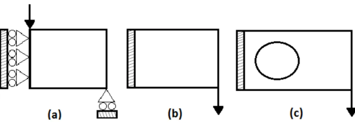
By taking different boundary conditions and making some changes in the code give rise to different topology optimization problems such as half of the "MBB beam", short cantilever beam and cantilever beam with a fixed circular hole. For all three optimization problems, the vertical unit force is shown in the Figure (2.1). Supports are implemented by eliminating fixed degrees of freedom from the linear equation which are obtained by finite element method. Both nodes and elements are num-bered column wise from left to right. For each iteration in the topology optimization loop, the code generates a picture of the current density distribution depending on the boundary conditions.
In MMA the move limit parameter is "0.2" for all problems. By taking move limit parameter "1.0" one gets Svanberg’s original MMA, the only purpose to choose move limit parameter "0.2" is to get a more stable solution process. In order to get a better convergent solution for both optimality techniques "0.01" termination criterion is used. It is observed that when these topology optimization problems are solved with MMA and OC, the optimality technique MMA took less iterations as compared to OC but CPU-time increased per iteration.
CHAPTER 2. TOPOLOGY OPTIMIZATION PROBLEM FOR COMPLIANCE MINIMIZATION
Figure 2.1. (a) Half MBB beam, (b) Short cantilever beam, (c) Cantilever beam
with a fixed hole.
2.6.1 Half MBB beam
The simply-supported Messerschmitt-Bölkow-Blohm (MBB) Beam: half design do-main with symmetry boundary conditions shown in the Figure (2.1(a)) is optimized for minimum compliance. Due to the overall symmetry, the computational model represents one half of the physical domain. The following boundary condition leads to the half MBB Beam problem.
F(2, 1) = −1; (2.7)
fixeddofs = union([1 : 2 : 2 ∗ (nely + 1)], [2 ∗ (nelx + 1) ∗ (nely + 1)]); The load is applied vertically in the upper left corner and there is symmetric boundary condition along the left edge and the structure is supported horizontally in the lower right corner.
Input line is: (nelx, nely, volfrac, penal, rmin) = (60, 20, 0.5, 3.0, 1.5),
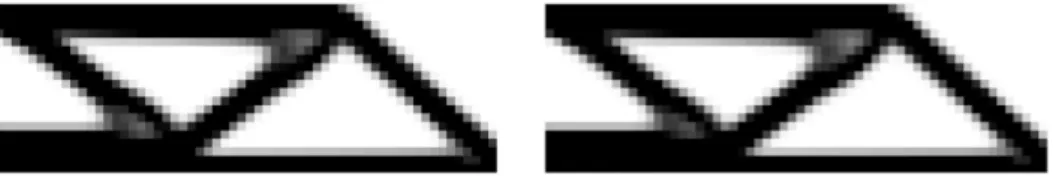
where nelx and nely are the number of elements in the horizontal and vertical di-rections, respectively, volfrac is the volume fraction, penal is the penalization power, rmin is the filter size (divided by element size) [19]. The topology optimization problem for half MBB beam solved with OC and MMA is shown in Figure (2.2). The filtered optimal topology of OC is obtained after 94 iterations with objective value 203.3061 whereas in case of MMA it takes 70 iterations with objective value 203.2381.
2.6. TOPOLOGY OPTIMIZATION PROBLEMS
Figure 2.2. Half MBB beam solved by OC on left and MMA on right
Figure 2.3. Short cantilever beam solved by OC on left and MMA on right
2.6.2 Short cantilever beam
For short cantilever beam optimization problem as shown in the Figure (2.1(b)), the boundary condition is:
F(2 ∗ (nelx + 1) ∗ (nely + 1), 1) = −1; (2.8) fixeddofs = [1 : 2 ∗ (nely + 1)];
where the command F(2, 1) = −1 is a vertical unit force in the lower right corner and fixeddofs are the fixed degrees of freedom. The Figure (2.3) shows the compari-son of cantilevered beam with those based on the OC method on the left and MMA on the right for 40% volume. The results are based on the filtering radius of r = 1.2. In case of OC, 71 iterations are used to optimize the problem having objective value 57.3492 whereas in case of MMA 50 iterations are needed to have an optimal solu-tion of objective value 57.2722.
CHAPTER 2. TOPOLOGY OPTIMIZATION PROBLEM FOR COMPLIANCE MINIMIZATION
Figure 2.4. Cantilever beam with a fixed hole solved by OC on left and MMA on
right
2.6.3 Cantilever beam with a fixed hole
In the optimal topology for a cantilevered beam with a fixed circular hole as shown in the Figure (2.1(c)) some of the elements may be required to take the minimum density value. The hole is modeled using passive elements with a circle of radius nely/3. and center (nely/2., nelx/3.). The zeros at elements free to change and ones at elements fixed to be zero. The load is applied vertically in the lower right corner.
The added lines are:
x(find(passive)) = 0.001; for ely = 1 : nely
for elx = 1 : nelx
if q(ely − nely/2.)2+ (elx − nelx/3.)2 < nely/3.
passive(ely, elx) = 1; x(ely, elx) = 0.001; else passive(ely, elx) = 0; end end end
Figure (2.4) shows the comparison of OC on the left with MMA on the right. In case of OC the total number of iterations are 34 having objective value 52.1080 whereas in case of MMA it takes 22 iterations with objective value 53.0281. The resulting structure obtained with the input:
(nelx, nely, volfrac, penal, rmin) = (45, 30, 0.5, 3.0, 1.5).
2.7. CONTINUATION PROCEDURE
By solving the three topology optimization problems, it is observed that the optimal solution by both methods are almost the same but OC works better than MMA. This is because, OC is developed for these kind of problems where only single constraint is involved and secondly the filter which is used here do not calculate the derivatives exactly "correct". So may be MMA is more sensitive to such kind of filter than that of OC.
2.7
Continuation procedure
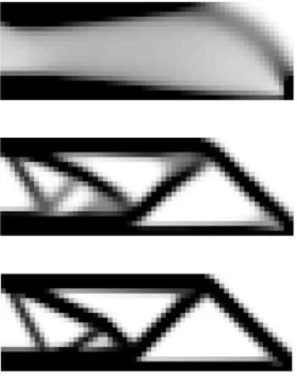
The purpose to solve topology optimization problem by using continuation proce-dure is to show the effect of penalization parameter by taking its value p = 1, 2 and 3. The continuation procedure is to start the problem by taking penalization parame-ter p = 1. Solve the problem to get the optimal solution. Let this optimal solution be the starting point of the problem for penalization parameter p = 2. Then solve the problem again and let the optimal solution be the starting point of the problem for penalization parameter p = 3. Solve this problem to get the final result. Figure (2.5) to (2.7) schematically shows the evolution of the topology during optimization process with MMA.
2.8
Results and Discussion
All three topology optimization problems which are stated in section (2.6) are solved by continuation procedure using method of moving asymptotes based optimizer.
2.8.1 MBB beam
A simply-supported Half MBB beam (2.7) with (nelx, nely, volfrac, penal, rmin) = (60, 20, 0.5, 3.0, 1.5), is optimized by continuation procedure using MMA is shown in the Figure (2.5). For p = 1 the number of iterations are 6 and the objective value is 164.7850, for p = 2 it takes 33 iterations to give optimal solution having objective value 199.3333. Finally, for p = 3 the number of iterations are 8 with objective value 203.1884.
2.8.2 Short cantilever beam
Short cantilever beam (2.8) is optimized with the same input as used in (2.6.2). For p = 1 the number of iterations are 6 and the objective value is 45.5047, for p = 2 it
CHAPTER 2. TOPOLOGY OPTIMIZATION PROBLEM FOR COMPLIANCE MINIMIZATION
Figure 2.5. Half MBB beam solved by continuation procedure with MMA
Figure 2.6. Short cantilever beam solved by continuation procedure with MMA
takes 19 iterations to give optimal solution having objective value 55.9763. Finally, for p = 3 the number of iterations are 12 with objective value 57.1348 shown in the Figure (2.6).
2.8. RESULTS AND DISCUSSION
Figure 2.7. Cantilever beam with a fixed hole solved by continuation procedure
with MMA
2.8.3 Cantilever beam with a fixed hole
Cantilever beam with a fixed circular hole is optimized by continuation procedure with those based on the MMA for a volume fraction of 50%. The results are based on the filtering radius of r = 1.5 (see 2.6.3). For p = 1 the number of iterations are 6 and the objective value is 49.6115, for p = 2 it takes 13 iterations to give optimal solution having objective value 51.5592. Finally, for p = 3 the number of iterations are 19 with objective value 53.0281 shown in the Figure (2.7).
By solving the three topology optimization problems, it is observed that in order to obtain true 0-1 (i.e. white and black) design the penalization parameter p = 3 is required. For this choice of p the intermediate densities are penalized as it is clearly seen in all the three Figures (2.5) to (2.7).
Chapter 3
Comparison of SIMP model and
alternative model
3.1
Introduction
In this chapter, An alternative interpolation scheme developed by Stolpe M and Svanberg K [21]; for minimum compliance topology optimization is compared with SIMP model. The implemented algorithm for both model is method of moving asymptotes. All three topology optimization problems of previous chapter half MBB beam, short cantilever beam and cantilever beam with a fixed hole are discussed here.
3.2
SIMP model
In SIMP (Solid Isotropic Material with Penalization) approach, a nonlinear inter-polation model for the material properties in terms of selection field is used. For each element, material properties are assumed constant and used to discretize the design domain. This interpolation is essentially a power law (3.1) that interpolates the Young’s modulus of the material to the scalar selection field, where the binary constraints are relaxed and intermediate values are penalized by replacing xj by
xpj for some given parameter p varies between [1, 3], in general, in the equilibrium equations. The intermediate values give very little stiffness in comparison to the amount of material used. The penalized compliance cp(x) in SIMP does not nec-essarily become a concave function, no matter how large p is chosen [22]. For the
CHAPTER 3. COMPARISON OF SIMP MODEL AND ALTERNATIVE MODEL
two-material problem the SIMP interpolation model can be expressed as:
Ep(xj) = E0+ xpj4E
satisfies Ep(0) = E0, Ep(1) = E1.
(3.1)
where 4E = E1− E0, while E0 and E1 are the Young moduli and it is assumed that E1 > E0 > 0. For a given parameter p ≥ 1, the SIMP problem is defined as:
min x∈Xp cp(x) = fTKp(x)−1f , where Kp(x) = n X j=1 Ep(xj)Kj.
3.3
Alternate model
Also in the alternate material model, the approach is to relax the zero-one con-straints and model the material properties by a law which gives non-integer solutions very little stiffness in comparison to the amount of material used. It was proved in [21]; that in this model the penalized compliance cq(x) becomes a concave function for sufficiently large q. For the two-material problem the alternative interpolation model can be expressed as:
Eq(xj) = E0+ xj/(1 + q(1 − xj))4E. (3.2)
satisfies Eq(0) = E0, Eq(1) = E1. (3.3)
where q is a penalty parameter, cq(x) is convex for q = 0 and concave for
q ≥ 4E/E0, see [21]. The penalized problem is defined as:
min x∈Xp cq(x) = fTKq(x)−1f , where Kq(x) = n X j=1 Eq(xj)Kj.
Let Eq(xj) denote the alternative interpolation model defined in (3.3) for a parameter q ≥ 0, i.e., Eq(xj) = E0+ xj (1 + q(1 − xj)) 4E. (3.4) 20
3.4. RESULTS AND DISCUSSION Differentiating Eq(xj) gives: Eq0(xj) = 4E(1 + q) [1 + q(1 − xj)]2 > 0 (3.5) and Eq00(xj) = 2q4E(1 + q) [1 + q(1 − xj)]3 ≥ 0. (3.6)
One of the major differences between the SIMP model and the alternative model is the behavior of the derivative of the material model at xj = 0, [21]. Evaluating the derivative of the alternative model and SIMP model at zero and one and comparing them shows that Ep0(0) is discontinuous in SIMP model in the parameter p whereas
Eq0(0) is continuous in the parameter q in alternative model.
Eq0(0) = 1 1 + q4E > 0 and E 0 q(1) = (1 + q)4E. (3.7) Ep0(0) = ( 4E if p = 1, 0 if p > 1, and Ep0(1) = p 4E. (3.8)
3.4
Results and Discussion
The topology optimization problems which discussed in chapter 2 solved again. Here considered four different scenarios, these problems are solved for SIMP model and also with alternate model objective function. And then considered alternate model and also solved with SIMP model objective function. The optimization technique used is method of moving asymptotes for all the possible cases.
3.4.1 MBB beam
Topology optimization problem of half MBB beam is solved for alternate model with penalized compliance q = 9.0, and in case of SIMP model penalization parameter is p = 3.0. The results obtained by both models is shown in the Table (3.1).
CHAPTER 3. COMPARISON OF SIMP MODEL AND ALTERNATIVE MODEL
Model SIMP objective function
Alternate objec-tive function
SIMP 203.2381 220.8406
Alternate 194.0418 205.9436
Table 3.1. Half MBB beam with alternate model and SIMP model
Model SIMP objective function
Alternate objec-tive function
SIMP 57.2722 61.0940
Alternate 53.8452 61.9126
Table 3.2. Short cantilever beam with alternate model and SIMP model
Model SIMP objective function
Alternate objec-tive function
SIMP 53.0281 56.2405
Alternate 51.3723 53.0245
Table 3.3. Cantilever beam with a fixed hole with alternate model and SIMP model
3.4.2 Short cantilever beam
When short cantilever beam is solved for alternate model with penalized compliance q = 9.0 and penalization parameter is p = 3.0 in case of SIMP model, the results obtained are shown in Table (3.2).
3.4.3 Cantilever beam with a fixed hole
Topology optimization problem of cantilever beam with a fixed hole is solved for alternate model with penalized compliance q = 9.0 and in case of SIMP model pe-nalization parameter is p = 3.0. The results obtained by both models is shown in the Table (3.3).
It is observed that in the three studied topology optimization problems, the obtained structures are very similar for both models in all cases. The optimal solution is slightly better for alternate model with SIMP model objective function for all three problems.
3.4. RESULTS AND DISCUSSION
Figure 3.1. Half MBB beam solved with alternate model
Figure 3.2. Short cantilever beam solved with alternate model
Chapter 4
Four node square elements, nine node
square elements and six node hexagonal
elements
4.1
Introduction
The purpose of this chapter is to compare three different types of finite elements for topology optimization. The reason of using nine node square elements and six node hexagonal elements is because of the checkerboard pattern that appeared in square four node elements when solved without filter. It is showed by Diaz AR and Sigmund O [6]; that the checkerboard pattern occurs because it has a numerically induced (artificially) high stiffness compared with a material with uniform material distribution. So possible ways to prevent checkerboard is to use some filter technique or to use higher order elements. This, however, increases the computational time.
4.2
Finite elements used
In this part of the report, the finite element equations for the stress analysis sub-jected to some external loads and support is solved. As discussed earlier, for sim-plicity all numerical examples in this thesis are two-dimensional. Therefore, the element used for the structural problems where the loading and the deformation occur within the plane is called a 2D solid element. In our case 2D solid element is square in shape for four node with bilinear shape functions and nine node with quadratic shape functions therefore the edges are straight as shown in Figure (4.4
CHAPTER 4. FOUR NODE SQUARE ELEMENTS, NINE NODE SQUARE ELEMENTS AND SIX NODE HEXAGONAL ELEMENTS
(a)). In case of six node it is hexagonal element with Wachspress shape functions. Order of the shape functions are used to determined the order of the 2D element. The equation system for 2D have following three steps:
1. Construction of shape functions matrix N that satisfies Delta function prop-erty and Partition of unity (Appendix A.3.1).
2. Formulation of the strain matrix B.
3. Calculation of stiffness matrix keby using shape function N and strain matrix
B in Eq. (A.4).
4.3
Four node square element
For square four node element the domain is discretized into a number of square
elements with four nodes and four straight edges. The nodes are numbered in counter-clockwise direction in each element as 1, 2, 3 and 4. The number of possi-ble directions that displacements or forces at a node can exist in is termed a degree
of freedom (DOF). The degrees of freedom (DOF) for each node is two, therefore
the total number of DOF is eight for square four node element.
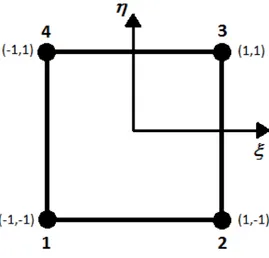
A local natural coordinate system (ξ, η) is defined with its origin located at the center of the element is shown in the Figure (4.1). The local node numbering is also shown in it. As discussed above, the very first task is to construct shape functions and that can be found in Appendix (B.1) for square four node. The shape functions satisfied the delta function property and partition of unity. The next step is to derive strain matrix required for computing the stiffness matrix of the element. The strain matrix is obtained with the use of shape function as: B = LN, where L is differential operator (see Appendix A.4). Once the shape function and strain matrix is obtained, the element stiffness matrix ke is obtained with the use
of equation (A.4).
4.4
Nine node square element
In case of square nine node element, the domain is discretized into a number of
square elements with nine nodes and four straight edges. The nodes are numbered
in counter-clockwise direction in each element as 1, 2, 3 and 4 on the corner of the square element. 5, 6, 7 and 8 are in the middle of the edges whereas 9 is in the
4.5. SIX NODE HEXAGONAL ELEMENT
Figure 4.1. The finite element four node in local coordinates (ξ, η). The local node
numbering is also shown.
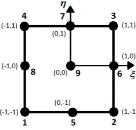
center of the element as shown in the Figure (4.2). The degrees of freedom (DOF) for each node is two, therefore the total number of DOF are 18 for each square nine node element.
Similarly, as in case of square four node a local natural coordinate system (ξ, η) is defined for square nine node with its origin located at the center of the element as shown in Figure (4.2). The local node numbering is also shown here. The shape functions constructed for square nine node can be found in Appendix (B.2). These shape functions also satisfies the delta function property and partition of unity. The strain matrix is obtained with the use of shape functions. After getting shape functions and strain matrix, the element stiffness matrix ke is calculated.
4.5
Six node hexagonal element
Six node hexagonal element (honeycomb) is one of the feasible alternative to avoid checkerboard pattern with Wachspress shape functions [27]. In our case mesh is uniform, so any two hexagonal elements that share an edge have two common ver-tices as shown in Figure (4.3). Thus there are two-node connections in hexagonal element which means that the two elements are either connected by two nodes or not connected at all. So it excludes the unwanted formation of checkerboard without
CHAPTER 4. FOUR NODE SQUARE ELEMENTS, NINE NODE SQUARE ELEMENTS AND SIX NODE HEXAGONAL ELEMENTS
Figure 4.2. The finite element nine node in local coordinates (ξ, η). The local node
numbering is also shown.
imposing any further restrictions (like filtration). The other feature of having uni-form mesh is that there are three edge-based symmetry lines per element as shown in Figure (4.4 (b)). This aspect allow to suffers less from directional constraint and allows for a more flexible arrangement of the final layout in the optimization process.
In this thesis Wachspress shape functions are used for hexagonal element (see Appendix B.3). These shape functions are bounded, non-negative and form a par-tition of unity. And also satisfy delta function property (A.3.1). For numerical integration, fully symmetric quadrature rules are developed for regions with regular hexagonal symmetry [26]. The list of quadrature points for various values of j can be found in Appendix (C.2).
4.6
Results and Discussion
The topology optimization problem for compliance minimization is solved for four node square elements with filter and without filter, nine node square elements and six node hexagonal elements with method of moving asymptotes based optimizer. In MMA move limit parameter "0.2" is used for all the cases to get a slightly more stable solution process in comparison with move limit "1.0". For all the three types of finite elements 40% volume and 50% volume taken into consideration, the penalization parameter, p, is 3 and the number of elements used to discretize the
4.6. RESULTS AND DISCUSSION
Figure 4.3. Square element mesh can display one node-connection while in a
hexag-onal mesh two connected elements always share two nodes through as edge connection
Figure 4.4. The square element has two edges-based-symmetry lines whereas
CHAPTER 4. FOUR NODE SQUARE ELEMENTS, NINE NODE SQUARE ELEMENTS AND SIX NODE HEXAGONAL ELEMENTS
Figure 4.5. Design Domain, loads and support for square element (a) and hexagonal
element (b)
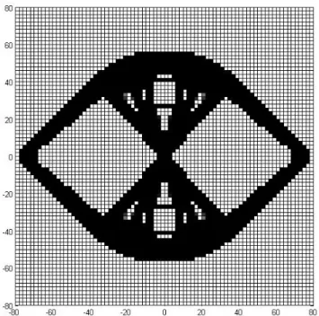
design domain, N, is 60×60 and 80×80. The structure is supported in the middle of the left and right sides not on the boundary of the structure but a little on the inside element of the structure which are fixed in both vertical and horizontal directions. The load is applied in the central element as shown in the Figure (4.5).
For four node square elements and nine node square elements when we say 40% volume and 50% volume it means 26% volume and 32.5% volume, respectively. The reason is that 40% of the hexagonal design space, in for example Figure (4.9), cor-responds to 26% of the square design space, in for example Figure (4.6) so that the area covered by the square finite element is comparable with the area covered by hexagonal finite element.
For a fair comparison of the three finite elements, the topology optimization problem is also solved for 100% volume for hexagonal finite element and 65% vol-ume for square finite elements (with the same reason as mentioned above) to get a black solution. Then taking the ratio of the compliance of obtained optimal solution for both 40% and 50% volume by the compliance of obtained black solution for all finite elements. This calculation is also shown in the Tables (4.1), (4.2), (4.3) and (4.4).
Another topology optimization problem is obtained by tilting the load (0, −1) in the center of the element to (−1/2, −1) while all the other parameters remains the same can be seen in Figure (4.5). The problem is solved for all the three finite
4.6. RESULTS AND DISCUSSION
Finite Elements Filter Number of iterations Optimal solution / Black solution Four node No 34 2.3512 Yes 76 2.3000 Nine node No 39 2.2159 Six node No 35 2.1049
Table 4.1. Volume 40%, Number of elements 60 × 60
elements with 40% volume and 50% volume and the number of elements used to discretize the design domain is 80 × 80.
4.6.1 40% Volume
Case I - 60×60
In Case I, the number elements used to discretize the design domain for 40% volume is 60 × 60. The topology optimization problem is solved with all the three finite elements are shown in Figures (4.6, 4.7, 4.8, 4.9). The results obtained by solving topology optimization problem is shown in Table (4.1).
CHAPTER 4. FOUR NODE SQUARE ELEMENTS, NINE NODE SQUARE ELEMENTS AND SIX NODE HEXAGONAL ELEMENTS
Figure 4.6. Four node square elements without filter; Volume 40%, N = 60 × 60
Figure 4.7. Four node square elements with filter; Volume 40%, N = 60 × 60
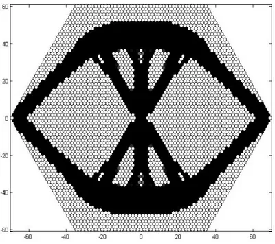
4.6. RESULTS AND DISCUSSION
Figure 4.8. Nine node square elements; Volume 40%, N = 60 × 60
CHAPTER 4. FOUR NODE SQUARE ELEMENTS, NINE NODE SQUARE ELEMENTS AND SIX NODE HEXAGONAL ELEMENTS
Finite Elements Filter Number of iterations Optimal solution / Black solution Four node No 29 2.2544 Yes 72 2.2018 Nine node No 44 2.1618 Six node No 32 1.9734
Table 4.2. Volume 40%, Number of elements 80 × 80
Figure 4.10. Four node square element without filter; Volume 40%, N = 80 × 80
Case II - 80×80
In Case II, the number of elements used to discretize the design domain is 80 × 80 while volume remain the same. By solving the topology optimization problem for four node square elements (with and without filter), nine node square elements and six node hexagonal elements the results obtained are shown in Table (4.2). The picture generated while solving the three finite elements are shown in Figures (4.10, 4.11, 4.12, 4.13).
4.6. RESULTS AND DISCUSSION
Figure 4.11. Four node square element with filter; Volume 40%, N = 80 × 80
CHAPTER 4. FOUR NODE SQUARE ELEMENTS, NINE NODE SQUARE ELEMENTS AND SIX NODE HEXAGONAL ELEMENTS
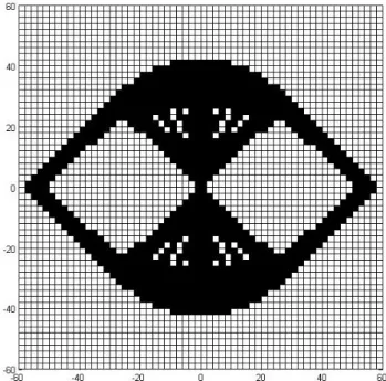
Figure 4.13. Six node hexagonal element; Volume 40%, N = 80 × 80
Finite Elements Filter Number of iterations Optimal solution / Black solution Four node No 41 1.8158 Yes 52 1.8103 Nine node No 32 1.7230 Six node No 32 1.6517
Table 4.3. Volume 50%, Number of elements 60 × 60
4.6.2 50% Volume
Case I - 60×60
In Case I, the number elements used to discretize the design domain for 50% vol-ume is 60 × 60. The topology optimization problem is solved with all the three finite elements are shown in Figures (4.14, 4.15, 4.16, 4.17). The results obtained by solving topology optimization problem is shown in Table (4.3).
4.6. RESULTS AND DISCUSSION
Figure 4.14. Four node square elements without filter; Volume 50%, N = 60 × 60
CHAPTER 4. FOUR NODE SQUARE ELEMENTS, NINE NODE SQUARE ELEMENTS AND SIX NODE HEXAGONAL ELEMENTS
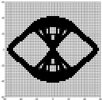
Figure 4.16. Nine node square elements; Volume 50%, N = 60 × 60
Figure 4.17. Six node hexagonal elements; Volume 50%, N = 60 × 60
4.6. RESULTS AND DISCUSSION
Finite Elements Filter Number of iterations Optimal solution / Black solution Four node No 28 1.7791 Yes 156 1.7661 Nine node No 42 1.7034 Six node No 39 1.5844
Table 4.4. Volume 50%, Number of elements 80 × 80
Figure 4.18. Four node square elements without filter; Volume 50%, N = 80 × 80
Case II - 80×80
In Case II, the volume remain the same but number of elements increased to 80 × 80 to discretize the design domain. The results obtained by solving the topology op-timization problem with four node square elements (with and without filter), nine node square elements and six node hexagonal elements are shown in Table (4.4). The picture generated in this case are shown in Figures (4.18, 4.19, 4.20, 4.21).
As discussed before, two elements in a hexagonal mesh either share one edge or not connected at all. Therefore, the geometric nature of hexagon Wachspress
CHAPTER 4. FOUR NODE SQUARE ELEMENTS, NINE NODE SQUARE ELEMENTS AND SIX NODE HEXAGONAL ELEMENTS
Figure 4.19. Four node square elements with filter; Volume 50%, N = 80 × 80
Figure 4.20. Nine node square elements; Volume 50%, N = 80 × 80
4.6. RESULTS AND DISCUSSION
Figure 4.21. Six node hexagonal elements; Volume 50%, N = 80 × 80
element can eliminate the severe error in the density representation that is observed with four node square elements in the form of checkerboard when solved without filter. Although the more accurate approximation of the displacement field may resolve the checkerboard problem for nine node square elements, but they may also suffer from one node hinges. With hexagonal mesh undesired small scale patterns may also be possible but still Wachspress element are more stable element for topol-ogy optimization.
As it is observed in all the cases that for four node square element checkerboard pattern appeared when it is solved without filter. Checkerboard pattern is avoided by using filtration. For nine node square elements and six nodes hexagonal elements no filtration is required and the resulting solid-void solution satisfies the imposed volume but in both cases a number of holes are observed. By taking the ratio of the compliance optimal solution to the compliance of black solution it is observed that six node hexagonal elements gives the lowest value in all the scenarios, so one can say that it gives a better optimal solution. Nine node square elements are better than four node square element with filter.
CHAPTER 4. FOUR NODE SQUARE ELEMENTS, NINE NODE SQUARE ELEMENTS AND SIX NODE HEXAGONAL ELEMENTS
To solve the topology optimization problem we used a machine with MATLAB version 7.10.0.499 (R2010a), 64-bit. The CPU is a Intel Core i3 M330 @ 2.13 GHz with 2.00 GB of 2.13 GHz RAM and observed that the nine node square elements are very expensive in computation as at least 200 minutes was taken by machine. For six node hexagonal elements 180 minutes, for four node square elements with filter 150 minutes and for four node square elements without filter 120 minutes.
We also solved the topology optimization problem by fixing the supports only in vertical direction and are free to move horizontally, while the load is applied vertically and fixed horizontally. All the three finite elements are solved for 40% and 50% volume, by taking penalization parameter p = 3, number of elements used to discretize the design domain are 60 × 60 and 80 × 80. The results are almost the same as calculated previously.
4.7
Another load condition
In order to obtained another optimization problem the load which is at (0, −1) in the center of the element changed by tilting it to (−1/2, −1) while the supports remains the same. All the three finite elements are solved for 40% volume and 50% volume, penalization parameter p is 3, the number of elements used to discretize the design domain is 80 × 80.
4.7.1 40% Volume - 80×80
In Case of 40% volume the topology optimization problem is solved for four node square elements (with and without filter), nine node square elements and six node hexagonal elements and the results obtained are shown in Table (4.5). The picture generated for all the cases can be seen in Figures (4.22, 4.23, 4.24, 4.25).
4.7. ANOTHER LOAD CONDITION
Finite Elements Filter Number of iterations Optimal solution / Black solution Four node No 52 2.1879 Yes 131 2.2489 Nine node No 52 2.1696 Six node No 39 2.0777
Table 4.5. Volume 40%, Number of elements 80 × 80
CHAPTER 4. FOUR NODE SQUARE ELEMENTS, NINE NODE SQUARE ELEMENTS AND SIX NODE HEXAGONAL ELEMENTS
Figure 4.23. Four node square elements with filter; Volume 40%, N = 80 × 80
Figure 4.24. Nine node square elements; Volume 40%, N = 80 × 80
4.7. ANOTHER LOAD CONDITION
CHAPTER 4. FOUR NODE SQUARE ELEMENTS, NINE NODE SQUARE ELEMENTS AND SIX NODE HEXAGONAL ELEMENTS
Finite Elements Filter Number of iterations Optimal solution / Black solution Four node No 42 1.7413 Yes 177 1.7721 Nine node No 54 1.6823 Six node No 48 1.6130
Table 4.6. Volume 50%, Number of elements 80 × 80
Figure 4.26. Four node square elements without filter; Volume 50%, N = 80 × 80
4.7.2 50% Volume - 80×80
In Case of 50% volume the topology optimization problem is solved for all the three finite elements as shown in Figures (4.26, 4.27, 4.28, 4.29). The results obtained by solving topology optimization problem is shown in Table (4.6).
When topology optimization problem is solved for another load condition it is observed that for four node square elements checkerboard pattern appeared when it is solved without filter and is avoided by using filtration. Also in this case six nodes hexagonal elements works better than the nine node square elements and four
4.7. ANOTHER LOAD CONDITION
Figure 4.27. Four node square elements with filter; Volume 50%, N = 80 × 80
CHAPTER 4. FOUR NODE SQUARE ELEMENTS, NINE NODE SQUARE ELEMENTS AND SIX NODE HEXAGONAL ELEMENTS
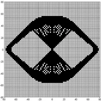
Figure 4.29. Six node hexagonal elements; Volume 50%, N = 80 × 80
node square elements with filter. As it can be seen from the Tables (4.5) and (4.6) that the ratio of the compliance of obtained optimal solution by the compliance of obtained black solution is less for six nodes hexagonal elements. But for such loading conditions a lot of holes appeared in six node hexagonal elements and nine node square elements. One can use filtration to remove these holes, but we left it for future work. In terms of time computation nine node square elements are still very expensive as compared to other two finite elements. Six nodes hexagonal elements takes much computation time than four node square elements with filter.
Chapter 5
Conclusion and future work
In this thesis topology optimization problems for minimum compliance solved with SIMP approach for four node square elements with bilinear shape function, nine node square elements with quadratic shape function and six node hexagonal ele-ments with Wachspress shape function.
5.1
Conclusion
The optimality techniques OC is compared with MMA solved for four node finite element with filter for three different topology optimization problems, namely half of the MBB beam, short cantilever beam and cantilever beam with a fixed hole. It is observed that MMA converge faster than OC but it takes much computation time per iteration. However, for such of kind of problems where a single constraint is involved OC works better and also by using gradient filtration technique the filtered derivatives are not exactly the correct derivatives and may be MMA is sensitive to this.
The topology optimization problems for minimum compliance are solved for al-ternate model and also with the same model but SIMP model objective function and compared the results obtained with SIMP model and also when it is solved with alternate model objective function. It is observed that in three studied topol-ogy optimization problems, the obtained structures are very similar for all scenarios but optimal value is slightly better for alternate model with SIMP model objective function.
CHAPTER 5. CONCLUSION AND FUTURE WORK
Finally, all the three finite elements are compared for SIMP model with MMA based optimizer. When the problem is solved with four node square elements with-out filter checkerboard pattern appeared in all the cases. As checkerboard pattern have artificially high stiffness, we use filtration. For nine node square elements and six node hexagonal elements no filtering is required as such and the resulting solid-void solution satisfies the imposed volume. But when the loading conditions are changed by tilting it, a number of holes are observed in the obtained structures of nine node square elements and six nodes hexagonal elements.
In all the cases six node hexagonal element with Wachspress shape functions give a better structure and optimized solution than the other finite elements. Nine node square elements is better than four node square elements with filter but it is very expensive in computation and use up more computation resources. As far as computation time is concern for six node hexagonal elements and four node square elements, six nodes takes more computation time than four node square elements with filter.
5.2
Recommendations for future work
Topology optimization for minimum compliance is solved with three different finite elements. Further studies however required to improve the convergence, using fil-tration in nine node square elements and six node hexagonal elements to remove the holes. One can also try to solve more technically interesting optimization prob-lems. Four node square elements and nine node square elements may be extended to three-dimensional structures but six node hexagonal element is a challenge to do so.
Appendix A
Finite element method procedure
The Finite Element Method have following key steps in order to analyze solid bodies [11].
A.1
Domain discretization
The very first step is to divide the solid body into Ne elements. The procedure is called meshing, performed using pre-processor. The role of pre-processor is to generates unique numbers for all elements and nodes in a proper manner. An element is formed by connecting its nodes. All the elements together form the entire domain of the problem without any gap or overlapping. The density of mesh depends upon the accuracy required for analysis.
A.2
Displacement interpolation:
To make it convenient in formulating the FEM equations for elements, local coor-dinate system is used. Which is defined for an element in reference to the global coordinate system (A.2.1) that is defined for the entire structure. The displacement at points (x, y) within the element is a polynomial interpolation:
Uh(x, y) =
nd
X
i=1
Ni(x, y)di = N(x, y)de (A.1)
where h is approximation, nd is the number of nodes forming an element, di is
the unknown nodal displacement to be computed and expressed in a general form as dTi = {dT1, dT2, . . . , dTnf} where nf is the number of degrees of freedom at a node.
APPENDIX A. FINITE ELEMENT METHOD PROCEDURE
And the vector de is the displacement vector for the entire element, and has the form dTe = {dT1, dT2, . . . , dTnd}. N is a matrix of shape functions for the nodes in the element.
A.2.1 Local and Global coordinates
Forces, displacements and stiffness matrices are often derived and defined for an axis system local to the member i.e. the coordinates apply to a single object. However there exist an overall axis system for the structure as a whole called global coordinate system or structure coordinate system i.e. the coordinates apply to everything uniformly [7].
A.3
Construction of shape function:
Construction of shape function depends on the geometry of the problem. Here 1-Dimensional case is explained but it can be extended to 2-Dimensional and 3-dimensional as well. Consider an element with nd nodes at xi (i = 1, 2, . . . , nd),
for 1-Dimensional xT = {x}. The displacement component is approximated in the form of a linear combination of nd linearly-independent basis functions pi(x).
uh(x) =
nd
X
i=1
pi(x)αi = pT(x)α (A.2)
where uh is the approximation of the displacement component, pi(x) is the
basis function of monomials in the space coordinates x, αi is the coefficient for the monomial pi(x). The vector α is defined as:
αT = {α1, α2, . . . , αnd}
The basis function pi(x) in Eq. (A.2) for 1-Dimensional has the form:
pT(x) = {1, x, x2, x3, . . . , xp}
The coefficient αi in Eq. (A.2) can be calculated by solving Eq. (A.2) to be equal to the nodal displacements at the ndnodes of the element. At node i it is of
the following form:
di= pT(xi) α i = 1, 2, . . . , nd