Impact of Macroeconomic Variables on the Stock Market Prices of the Stockholm Stock Exchange (OMXS30)

(1)

J

Ö N K Ö P I N G

I

N T E R N A T I O N A L

B

U S I N E S S

S

C H O O L

JÖNKÖPING UNIVERSITY

Impact of Macroeconomic Variables on the Stock Market Prices of the

Stockholm Stock Exchange (OMXS30)

Master´s Thesis within International Financial Analysis

Author: Joseph Tagne Talla

Tutors: Per-Olof Bjuggren, Louise Nordström Jönköping May 2013

(2)

2

Acknowledgments

I would like to thank my supervisors Professor Per-Olof Bjuggren and Louise Nordström for their invaluable contributions.

(3)

3

Abstract

The key objective of the present study is to investigate the impact of changes in selected macroeconomic variables on stock prices of the Stockholm Stock Exchange (OMXS30). To estimate the relationship, unit root test, Multivariate Regression Model computed on Standard Ordinary Linear Square (OLS) method and Granger causality test have been used. The time period examined is 1993-2012 and all the tests are conducted based on monthly data. Based on estimated regression coefficients and t-statistics, it is found that inflation and currency depreciation have a significant negative influence on stock prices. In addition, interest rate is negatively related to stock price change, but it is not significant in the model. On the other hand, money supply is positively associated to stock prices although not significant. No unidirectional Granger Causality is found between stock prices and all the predictor variables under study except one unidirectional causal relation from stock prices to inflation.

Keywords: Macroeconomics variables, stock prices, OLS, Granger Causality test.

Master´s thesis in International Financial Analysis

Title: Impact of Macroeconomic Variables on the Stock Market Prices of the Stockholm

Stock Exchange

Author: Joseph Tagne Talla

Tutors: Per-Olof Bjuggren, Louise Nordström

(4)

4

Abbreviations

ADF……… Augmented Dickey-Fuller APT……… Asset Pricing Theory

CAPM……… Capital Asset Pricing Model OMXS30………... OMX Stockholm 30

(5)

5

1 Introduction ...Erreur ! Signet non défini.7

1.1 Limitations ... 7

1.2 Outline ... 8

2 Theoretical Framework ... 9

2.1 The Efficient Market Hypothesis ... 9

2.2 The Arbitrage Pricing Theory. ... 10

3 Literature Review ... 12

4 Data and Methodology ... 17

4.1 Variables description and Expectation ... 17

4.2 Data ... 19

4.3 Methodology ... 20

5 Empirical Results ... 22

5.1 Unit Root Test ... 22

5.2 Regression Output (OLS) ... 24

5.3 Residuals diagnostics ... 26

5.3.1 Correlogram for the Residuals... 26

5.3.2 Serial Correlation LM Test ... 27

5.3.3 Heteroscedasticity Test ... 28

5.3.4 Normality Test ... 28

5.3.5 Granger Causality Test ... 29

6 Discussion and Conclusion ... 31

6.1 Further Research... 31

7 References ... 33

8 Appendix ... 37

8.1 Appendix 1: ADF Test ... 37

8.1.1 Stock Price (OMXS30) ... 37

8.1.2 Consumer Price Index (CPI) ... 39

8.1.3 Money Supply (MS) ... 41

8.1.4 Interest Rate (IR) ... 44

(6)

6

8.2 Appendix 2: Eviews output Ordinary Linear Square Test ... 47 8.3 Appendix 3: Eviews output Granger Causality Tests ... 48

(7)

7

1 Introduction

A stock exchange market is the center of a network of transactions where buyers and sellers of securities meet at a specified price. Stock market plays a key role in the mobilization of capital in emerging and developed countries, leading to the growth of industry and commerce of the country, as a consequence of liberalized and globalized policies adopted by most emerging and developed government. Many factors can be a signal to stock market participants to expect a higher or lower return when investing in stock and one of these factors are macroeconomic variables. The change in macroeconomic variables can significantly impact stock price return.

The results of this empirical research help the reader to understand whether the movement of stock prices of the Stockholm Stock Exchange (OMXS30) is subject to some macroeconomic variables change. Investors will find this study as a helpful tool for them to identify some basic economic variables that they should focus on while investing in stock market and will have an advantage to make their own suitable investment decisions.

The present research considers four macroeconomic variables: Consumer Price Index (CPI) as proxy for inflation rate, Exchange Rate (ER), Money Supply (MS), Interest Rate (IR) and on the other hand Stockholm Stock Exchange indices in the form of OMXS30. In the study we use the Ordinary Least Squared (OLS) to test the impact of macroeconomic variables on Stockholm Stock Exchange Indices and vice versa (using the Granger causality test), based on monthly data from January, 1993 to December, 2012. Besides, Augmented Dickey-Fuller (ADF) test to check the stationarity of the data and diagnostic checking to check if residuals from the regression are white noise.

The objective of this paper is to investigate the impact of macroeconomic variables on the stock market prices of the Stockholm stock exchange during the period 1993-2012. This paper is a complement to the existing literature. To our knowledge, the present research is the most recent one that focuses on the Swedish stock market.

1.1 Limitations

Another three important macroeconomic variables that are commonly used in research to explain changes in stock prices have been excluded from the present paper namely: Industrial Production,

(8)

8

Foreign Exchange Reserves and Oil Prices variables. The exclusion of the Industrial Production and Oil Price variables was due to the lack of consistent data for the study period. However, the Foreign Exchange Reserves variable was negative and insignificant when included in the regression model and there was not previous research to attest to this finding of negative relationship between foreign exchange reserves and stock prices. Besides, this result can be explained by the fact that Sweden has a fluctuating exchange regime. Based on that, foreign exchange reserves variable was excluded from the model and its exclusion did not affect the regression and the residual diagnostic testing results.

1.2 Outline

The thesis is organized as follows. Section 2 reviews the theoretical framework with respect to both efficient market hypothesis and arbitrage pricing theory. Section 3 provides a literature review and gives support to the variables considered in this research. Section 4 describes the data and methodology used in the research. Section 5 focuses on the empirical results and discussions of ADF test, regression analysis, diagnostic checking and Granger causality test. Section 6 provides a discussion as well as suggestions for further research and concludes this research.

(9)

9

2 Theoretical Framework

Different theoretical frameworks have been employed by many researchers to link changes in macroeconomic variables with stock market returns. These include the semi strong efficient market hypothesis developed by Fama (1970) and the Arbitrage Pricing Theory (APT) developed by Ross (1976). These theories are discussed in this section as they relate the macroeconomic variables to stock market return.

2.1 The Efficient Market Hypothesis

Popularly known as random walk theory, the efficiency market hypothesis assumes that market prices should incorporate all available information at any point in time. The term “efficient market” was first used by Eugene Fama (1970) who said that: “in an efficient market, on the average, competition will cause the full effects of new information on intrinsic values to be reflected instantaneously in actual prices”. Fama defined an efficient market as “a market where prices always reflect all available information”. Indeed, profiting from predicted price movements is unlikely and very difficult as the efficient market hypothesis suggests that the main factor behind price changes is the arrival of new information.

However, there are different kinds of information that affect security values. Consequently, the efficient market hypothesis is stated in three variations namely: the weak form hypothesis, semi strong form hypothesis and the strong form hypothesis depending on what the term “available information” means.

This paper focuses on the semi strong hypothesis since it is the most convenient for our study. As a matter of fact, the semi strong hypothesis states that all publicly available information is already incorporated into current prices; that is the asset prices reflect all available public information. Indeed, the semi strong hypothesis is used to investigate the positive or negative relationship between stock return and macroeconomic variables since it postulates that economic factors are fully reflected in the price of stocks. Public information can also include data reported in a company´s financial statement, the financial situation of company´s competitors, for the analysis of pharmaceutical companies. Hence, information is public and there is no way to make profit using information that everybody else knows. So the existence of market analysts is required to be able to understand the implication of vast financial information as well as to comprehend processes in product and input market.

(10)

10

2.2 The Arbitrage Pricing Theory.

Developed by Ross (1976), the Arbitrage Pricing Theory (ATP) is another way of linking macroeconomic variables to stock market return. It is an extension of the Capital Asset Pricing Model (CAPM) which is based on the mean variance framework by the assumption of the process generating security. In other words, CAPM is based on one factor meaning that there is only one independent variable which is the risk premium of the market. There are similar assumptions between CAPM and APT namely: the assumption of homogenous expectations, perfectly competitive markets and frictionless capital markets.

However, Ross (1976) proposes a multifactor approach to explaining asset pricing through the arbitrage pricing theory (APT). According to him, the primary influences on stock returns are some economic forces such as (1) unanticipated shifts in risk premiums; (2) changes in the expected level of industrial production; (3) unanticipated inflation and (4) unanticipated movements in the shape of the term structure of interest rate. These factors are denoted with factor specific coefficients that measure the sensitivity of the assets to each factor. APT is a different approach to determining asset prices and it derives its basis from the law of one price. As a matter of fact, in an efficient market, two items that are the same cannot sell at different prices; otherwise an arbitrage opportunity would exits. APT requires that the returns on any stock should be linearly related to a set of indexes as shown in the following equation:

(1) Where

= the expected level of return for stock i if all indices have a value of zero = the value of the jth index that impacts the return on stock i

= the sensitivity of stock i´s return to the jth index

= a random error term with mean equals to zero and variance equal to

According to Chen and Ross (1986), individual stock depends on anticipated and unanticipated factors. They believe that most of the return realized by investors is the result of unanticipated events and these factors are related to the overall economic conditions. In fact, although asset returns can also be affected by influences that are not systematic to the economy, returns on large

(11)

11

portfolios are mainly influenced by systematic risk because idiosyncratic returns on individual assets are cancelled out through the process of diversification.

(12)

12

3 Literature Review

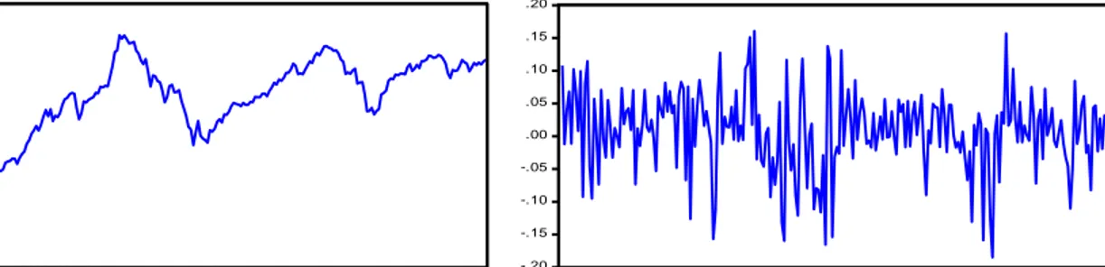
Founded in 1863, Stockholm Stock Exchange is the main securities market in Sweden. After merging with OMX in 1998, Stockholm Stock Exchange is held today by the Nordic division of the largest exchange holding company in the world, namely NASDAQ OMX. An overview of Stockholm Stock Price Index is represented on figure 1 from 1993 to 2012 (monthly representation). The measure of predictability and efficiency of stock returns has always been an interesting topic for researchers, investors and government agencies.

Figure 1: Stockholm stock Price Index (1993-2012)

Several researchers have centered their empirical studies on the relationship between stock market movement and macroeconomic variables and this has been intensively examined in both emerging and developed capital markets. Homa and Jaffe (1971), Hamburger and Kochin (1972) find a positive relationship between money supply and stock prices. This result follows the ideas of real activity economists who argue that if there is an increase in money supply; it means that money demand is increasing which is a signal of an increase in economic activity. This increase in economic activity implies higher cash flows, which causes stock prices to rise (Sellin, 2001).

Grossman and Shiller (1980) examine how historical movements can be justified by new information. Using historical data from 1890-1979, they show evidence that stock price movement can be attributed to real interest rate movement.

0 200 400 600 800 1,000 1,200 1,400 1,600 1994 1996 1998 2000 2002 2004 2006 2008 2010 2012

(13)

13

Another study is that of Chen, Roll and Ross (1986) who investigate the impact of macroeconomic variables on stock prices. They employ seven macroeconomic variables to test the multifactor model in the USA. They find that consumption market index and oil prices are not related to financial market while industrial production, change in risk premium and twist in the yield curve are significantly related to stock returns.

Gjerde and Saettem (1999) study the relation between stock returns and macroeconomic variables in Norway. Their results show a positive relationship between oil price and stock returns as well as real economic activity and stock returns. However, their study fails to show a significant relation between stock returns and inflation.

Bhattacharya et. al. (2001) analyze the causal relationship between the stock Market and three macroeconomic variables in India`s case using the Granger non-causality. These macroeconomic variables are: exchange rate, foreign exchange reserves and trade balance. The results suggest that there is no causal linkage between stock prices and the three variables under consideration.

In their study based on six Asian countries, Doong et al (2005) investigate the relationship between stocks and exchange rates using the Granger causality test. According to their results, there is a significantly negative relation between the stock returns and change in the exchange rates for all the included countries except one.

Uddin and Alam (2007) examine the linear relationship between share price and interest rate as well as share price and changes of interest rate. In addition, the also explore the association between changes of share price and interest rate and lastly changes of share price and changes of interest rate in Bangladesh. They find for all of the cases that Interest Rate has significant negative relationship with Share Price and Changes of Interest Rate has significant negative relationship with Changes of Share Price.

Geetha, Mohidin, Chandran and Chong (2011) investigate the relationship between stock market, expected inflation rate, unexpected inflation rate, exchange rate, interest rate and GDP in the case of Malaysia, US and China. They use cointegration test to determine the number of cointegrating vectors, which shows the long-run relationship between the variables while the short-run relationship was determined using the Vector Error Correction model. Their results indicate that there is a long run cointegration relationship between stock markets and those variables in

(14)

14

Malaysia, US and China. On the other hand, there is no short run relationship between the stock market, unexpected inflation, expected inflation, interest rate, exchange rate and GDP for Malaysia and US using VEC. However, China’s VEC result shows that there is a short-run relationship between expected inflation rates and China’s stock market.

Gay (2008) investigates the relationship between stock market index price and and the macroeconomic variables of exchange rate and oil price for emerging countries (Brazil, Russia, India, and China) using the Box-Jenkins ARIMA model. He finds no significant relationship between respective exchange rate and oil price on the stock market index prices in any of the emerging countries. He concludes that this result suggests that the markets of Brazil, Russia, India, and China exhibit the weak-form of market efficiency.

Mohammad (2011) uses Multivariate Regression Model computed on Standard OLS formula and Granger causality test to model the impact of changes in selected microeconomic and macroeconomic variables on stock returns in Bangladesh. He examines monthly data for all the variables under study covering the period from July 2002 to December 2009. The study finds a negative relationship between stock returns and inflation as well as foreign remittance while market Price/Earnings and growth in market capitalization have a positive influence on stock returns. However, no unidirectional Granger Causality is found between stock returns and any of the independent variables and the lack of Granger Causality reveals the evidence of an informally inefficient market.

Mahedi (2012) examines the long-run relationship and the short-run dynamics among macroeconomic variables and the stock returns of Germany and the United Kingdom. He uses the Johansen Co-integration test to indicate the co-integrating relationship between the stock prices and macroeconomic determinants. And then, he uses error-correction models to investigate both the short-and long-term casual relationships and each case is examined individually. For Germany case, the results show that the short-run causality runs from stock returns to inflation, from money supply to stock returns and from industrial production to stock returns. The long-run causality runs from inflation to stock returns and from exchange rate to stock returns. There is only one short-and long-run relationship, that is from the stock returns to industrial production. For the United Kingdom case, he finds that the short run causality run from stock returns to T-bill, from stock returns to money supply, from stock returns to exchange rate, exchange rate to

(15)

15

stock returns and stock returns to industrial production. The long run causality runs from inflation to stock returns. The short and long-run causal relationship runs from stock returns to inflation, from money supply to stock returns and from industrial production to stock returns. These results indicate the existence of short-run interactions and long term causal relationship between both Germany and the UK stock markets and the macroeconomic fundamentals.

Ray Sarbapriya (2012) uses a simple linear regression model and Granger causality test to measure the relationship between foreign exchange reserves and stock market capitalization in India. The results show that causality is unidirectional and it runs from foreign exchange reserve to stock market capitalization and that foreign exchange reserves have a positive impact on stock market capitalization in India.

Many other early studies of Lintner (1973), Jaffe and Mandelker (1977) and Fama and Schwert (1977) examine the relationship between inflation and stock prices. Most of these studies test the Fisher hypothesis which predicts a positive relationship between expected nominal returns and expected inflation and their findings are inconsistent with the Fisher hypothesis. They all report a negative linkage between stock returns and inflation. However, Firth (1979) observes a positive relationship between nominal stock returns and inflation when studying the relationship between stock market returns and rates of inflation in the United Kingdom.

Table 1: Impact of macroeconomic variables on stock market

Macroeconomic variables

Positive Negative Insignificant

Inflation Firth (1979) Lintner (1973)

Fama and Schwert (1977) Mandelker (1977) Geetha, Mohidin, Chandran and Chong (2011) Gjerde and Saettem (1999) Chen, Roll and Ross (1986)

Interest rate Uddin and Alam

(2007)

Geetha, Mohidin, Chandran and Chong (2011)

Exchange rate Geetha, Mohidin,

Chandran and Chong (2011) Doong et al (2005) Bhattacharya et. al.(2001) Robert D. Gay (2008)

(16)

16

Money Supply Homa and Jaffe

(1971)

Hamburger and Kochin (1972)

Mahedi (2012)

Oil price Gjerde and Saettem

(1999)

Chen, Roll and Ross (1986) Robert D. Gay (2008) Foreign exchange reserves Ray Sarbapriya (2012) Bhattacharya et. al.(2001)

Industrial production Mahedi (2012)

Chen, Roll and Ross (1986)

(17)

17

4 Data and Methodology

4.1 Variables description and Expectation

Dependent variable; OMX Stockholm 30 (OMXS30)

The OMX Stockholm 30 is a stock market index for the Stockholm Stock Exchange. It is the market value weighted index of the 30 stocks that have the largest trading volume on the Stockholm Stock Exchange.

Consumer Price Index (CPI)

Consumer price index is used as a proxy for inflation. The relationship between inflation and stock returns can be positive or negative depending on whether the economy is facing unexpected or expected inflation. Expected inflation happens when demand exceeds supply, causing an increase in prices to stimulate more supply. Since this is expected by the firms, increase in prices would also increase their earnings which would lead to them paying more dividends and hence increase the price of their stocks as well. On the other hand when inflation is unexpected, an increase in price will lead to the increase in cost of living and this will shift resources from investment to consumption. Indeed, as inflation increases, nominal interest rates will also increase. The discount rate used to determine intrinsic values of stocks will therefore increase, and thus this will reduce the present value of net income leading to lower stock prices. Moreover, if the price elasticity of demand for the firm´s products is high, a rise in inflation may cause a decline in a firm’s sales and net income, and thus its stock price.

This negative relationship between unexpected inflation and stock prices is hypothesized by Fama (1981) as a function of the relationship between unexpected inflation and real activity in the economy. This research is based on APT, which is built on the relationship between the unexpected changes in economy and stock returns, thus inflation is expected to be negatively associated to stock prices.

Interest Rate (IR)

The money market rate is considered as a proxy for interest rate. The money market is a segment of the financial market in which financial instruments with high liquidity and very short maturities are traded. The money market is used by participants as a means of borrowing and

(18)

18

lending in the short term, from several days to just under a year. An increase in the interest rate will result in falling stock prices due to the fact that high interest rate will increase the opportunity cost of holding money, causing substitution of stocks for interest bearing securities.

Interest rate is one of the important macroeconomic variables and is directly related to economic growth. From the point of view of a borrower, interest rate is the cost of borrowing money while from a lender’s point of view, interest rate is the gain from lending money. The interest rate is expected to be negatively associated to stock returns.

Exchange Rate (ER)

The next macroeconomic variable used in this study is the exchange rate which in this case is the bilateral nominal rate of exchange of the Swedish krona (SEK) against one unit of a foreign currency, Euro (€). The reason is that Eurozone countries are the main market for Swedish foreign trade. An increase in exchange rate (depreciation) will cause a decline in stock prices because of expectations of inflation. Moreover, heavy importer companies will suffer from higher costs due to a weaker domestic currency and will have lower earnings, and lower share prices. As a result, the stock market, which is a collection of a variety of companies, trends to react negatively to currency depreciation. However, domestic exporters benefit from currency depreciation because it causes domestic products to become cheaper to foreign clients. So on macroeconomic level, currency depreciation will boost the domestic export industry and depress the import industry. Overall, the effect of exchange rate on stock prices can be either a positive or a negative relationship. Based on Doong et al (2005) work, we assume the negative relationship is predominant.

Money Supply (MS)

The form of money supply called M0 is defined as the non-bank sectors holdings of notes and coins. It is calculated by subtracting the notes and coins held by banks from the total quantity of Riksbank notes and coins in circulation. An increase in the money supply is frequently assumed to positively affect stock prices. When money stock grows, it stimulates the economy which leads to greater credit being available to firms to expand production and then increases sale resulting in increased earnings for firms. This results in better dividend payments for firms leading to an increase in the price of stocks. However, money supply can also be negatively associated to stock prices. To illustrate this argument, we first go through the link between money supply and

(19)

19

inflation, since the expansion of the money supply is positively related to inflation in the economy which would increase the nominal risk free rate (Fama, 1981). This increase in the nominal risk free rate will lead to a rise in the discount rate which leads to a fall in return. A positive relationship between money supply and stock price is expected in this study.

Table 2: Regression Variables

Variables Explanations Data source and

Period

Expected sign of coefficient

Dependent variable

OMXS30 The OMX

Stockholm 30 is a stock market index for the Stockholm Stock Exchange, in Swedish Krona.

Nasdaq OMX, Jan 1993 - Dec 2012, monthly.

Na

Independent variables

CPI The Consumer Price

Index (CPI) is the most common measure of inflation. Index ranges from 0 to 100 with high rating means high inflation.

Statistics Sweden (SCB), Jan 1993 - Dec 2012, monthly.

-

IR Money market rate

as a proxy to interest

rate. Monthly

average of daily rates for day-to-day interbank loans (%) International Financial Statistics (IMF), Jan 1993 - Dec 2012, monthly. - ER Exchange rate, Swedish krona (SEK) against one unit of Euro (€). WM/Reuters, Jan 1993 - Dec 2012, monthly. - MS Money supply (M0), millions Swedish Krona. Sveriges Riksbank, Jan 1993 - Dec 2012, monthly. + 4.2 Data

The objective of this paper is to empirically examine the impacts of some macroeconomic factors on the stock market returns of the Stockholm stock exchange (OMXS30). In this study, stock price index (OMXS30) is considered as the dependent variable. On the other hand, based on

(20)

20

previous studies, four macro-economic variables namely Consumer Price Index (CPI), Call Money Rate (IR), Exchange Rate (ER) and Money Supply (MS) are used as predictor variables. The study examines monthly data for all the variables under study covering the period from January 1993 to December 2012 (240 monthly observations) which are collected from the Thomson Reuters FinancialDatastream.

Table 3 presents the summary of descriptive statistics for the selected dependent and independent variables under study. 240 monthly observations of all the variables have been examined to estimate the following statistics. The mean describes the average value in the series and Std. Deviation measures the dispersion or spread of the series. The maximum and minimum statistics

measures upper and lower bounds of the variables under study during our chosen time span.

Table 3: Descriptive statistics for 1993-2012

Mean Minimum Maximum Std.

Deviation LOMXS30 762,1750 174,1300 1433,080 308,3970 LCPI 275,8629 241,0000 315,4900 21,32207 LIR 3,895542 0,350000 10,90000 2,353708 LER 9,137867 8,139000 11,46000 0,519209 LMS 83 727,82 58 646,00 100 883,0 13 218,25 N 240 4.3 Methodology

Two main econometric models are conducted in this study: the Ordinary Least Squared (OLS) to test the relationship between the macroeconomic variables and the stock price index (OMXS30), and Granger Causality test to examine the relation between individual explanatory variables and OMXS30 (either unidirectional, bidirectional or no relation).

However, it is important to keep in mind that time series data analysis is subject to the problem of spurious regression if the data is non-stationary, resulting in unreliable results of the models constructed. So to avoid spurious regression, the unit root test (Augmented Dickey –Fuller test) will be conducted first to check if the time series data is stationary. If the test shows that the data is non-stationary, the first difference of the variables will be employed before conducting the

(21)

21

OLS method and the Granger Causality Test. The multivariate regression is developed in the following equation:

(2)

Firstly, all the variables under study are transformed into the logarithmic form. Then, because of the existence of a unit root in all the variables data series (Tables 4 and 5), the first difference of logarithm of all the variables and the second difference of the logarithm of money supply are used.

(22)

22

5 Empirical Results

5.1 Unit Root Test

When dealing with time series data, it is important to examine the existence of unit root in the data series. If the variable is not stationary, we can obtain a high although there is no meaningful relation between variables. A non-stationary process generates the problem of spurious regression between unrelated variables. Before running our linear regression and Granger causality test, we need to test for Unit root and make sure that we are dealing with stationary data before using it. There are numerous unit root tests and one of the most popular among them is the Augmented Dickey-Fuller (ADF) test. Augmented Dickey -Fuller (ADF) is an extension of Dickey -Fuller test.

The null and alternative hypotheses are as follows:

Unit root [Variable is not stationary] No unit root [Variable is stationary]

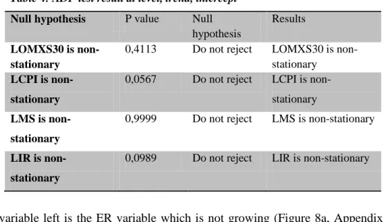
If the coefficient is significantly different from one (less than one) then the hypothesis that y contains a unit root is rejected. Rejection of the null hypothesis denotes stationarity in the series. If we don´t reject the null hypothesis, we conclude we have a unit root. Before running ADF test, we plot the variable to check if there is a trend and use the Elder and Kennedy unit root model selection approach. OMXS30, CPI MS and IR are growing as we can see respectively from figures 4a, 5a, 6a and 7a (Appendix 1). So the ADF test is run at level with trend and intercept as summarized in table 4.

By looking at the results, it appears that the p-values for all the included variables in our research are greater than the critical value (5%). So we cannot reject the null hypothesis and we must therefore conclude that four variables out of five which are growing are non-stationary, meaning that those variables follow a random walk with drift and no time trend. This implies that we need to take the first difference of those variables before they can be run in the regression model

(23)

23

The only variable left is the ER variable which is not growing (Figure 8a, Appendix 1). So we run the ADF test only at level, with intercept and no trend as we can see the result from table 5.

Table 5: ADF Test at level, intercept

LER 0,1356 Do not reject LER is non-stationary

Since the p-value (0.1356) is greater than the critical value (5%), we cannot reject the null hypothesis and we can conclude that ER variable is following a pure random walk.

Following the results from table 4 and 5, the remedy is to take the first difference of all the variables before using them in the regression model. Table 6 is the summary of such test. The p-values of four out of five variables included in our regression are less than the critical value (5%). In other words, the p-values of OMXS30, CPI, IR and EP are less than 5%, meaning that we reject the null hypothesis. We can conclude that those variables are stationary at first difference. It is easy to see that the trend on OMXS30, CPI and IR variables is removed when taking their first difference as we see in their respective figures 4b, 5b, 7b (Appendix 1).

However, the p-value for MS is greater than critical level, 25, 39% 5%, we cannot reject the null hypothesis and we conclude that MS is non-stationary at first difference and it follows a pure random walk at first difference since it is not growing (Figure 6b, Appendix 1).

Table 4: ADF test result at level, trend, intercept

Null hypothesis P value Null

hypothesis

Results

LOMXS30 is non-stationary

0,4113 Do not reject LOMXS30 is non-stationary

LCPI is non-stationary

0,0567 Do not reject LCPI is non-stationary

LMS is non-stationary

0,9999 Do not reject LMS is non-stationary

LIR is non-stationary

(24)

24

The results of ADF test at first difference conclude that all variables are stationary, except MS. So we need to run ADF test at second difference at level for MS variables since it follows a pure random walk at first difference. From table 7, we can see that the p-value (0%) is less than critical level (5%). We reject the null hypothesis and conclude that MS variable is stationary at second difference.

5.2 Regression Output (OLS) Our OLS equation is as follows:

Where D is the first difference and DD is the second difference. The model output is summarized in table 8.

Table 8: The Effects of Macroeconomic Variables on Stock Market Prices

Variable Coefficient t-Statistic Probability

C 0,008853 2,233070 0,0265

Table 6: ADF test at difference

Null hypothesis P-value Null

hypothesis

Results

LOMXS30 is not stationary

0,0000* Reject LOMXS30 is stationary

LCPI is not stationary

0,0135* Reject LCPI is stationary

LMS is not stationary 0,2539 Do not reject LMS is non-stationary

LER is not stationary 0,0000* Reject LER is stationary

LIR is not stationary 0,0002* Reject LIR is stationary

(*) means significant at 5% critical level

Table 7: ADF test at difference

Null hypothesis P value Null hypothesis Results

LMS is not stationary 0,0000* Reject LMS is

stationary

(25)

25 DLCPI – 2,066528 – 2,069061* 0,0396 DDLMS 0,119401 1,215672 0,2253 DLIR – 0,048940 – 1,043833 0,2976 DLER – 1,190890 – 5,493487* 0,0000 R-squared 0,128075 Adjusted R-squared 0,113106 F-statistic 8,556205 N 238

Note: DLOMXS30, DLCPI, DLIR and DLER denote the first difference of the log values of stock price index (OMXS30), consumer price index, interest rate, exchange while DDLMS denotes the second difference of the log value of money supply. (*) sign means significant at 5% critical level.

Table 8 presents the output of the Ordinary Least Square (OLS) method to show the impact of the macroeconomics variables on stock market prices. I can be noticed that both the predicted and all the predictor variables are log-transformed. This is associated with the price elasticity meaning that the percentage change in Y is caused by one percentage change in X. For example in the case of this study, 1% change in inflation will cause stock prices to decrease by 206%. The output from table 8 shows a significant relationship between inflation (DLCPI) and stock price index (since its p-value 0.0396 is less than 5%). The negative sign of the coefficients means that increase in inflation will cause stock price to fall. This is consistent with the previous evidence of a negative and significant linkage between inflation and stock returns (Lintner, 1973; Fama and Schwert, 1977). Another negative significant linkage is found between exchange rate and stock prices as it can be seen on its negative coefficient sign and its p-value (0.0000<0.05). This means that depreciation of currency will cause the stock price to fall and this result confirms early evidence (Doong et al, 2005). Although the other macroeconomic variables are not significant, their coefficient signs confirm our expectations. Indeed, the money supply coefficient is positive, meaning that an increase in money supply will cause the price to increase as well. The negative coefficient sign of the interest rate means that an increase in the interest rate will cause the stock price to decrease.

(26)

26

5.3 Residuals diagnostics

To confirm and trust the T-test results from our OLS regression, we have to make sure that the residuals are white noise. Residuals from a regression should never contain any systematic information, since this is a sign that this information is not included in the regression model.

5.3.1 Correlogram for the Residuals

Figure 2: correlogram for the Residuals

Date: 05/15/13 Time: 17:05 Sample: 1993M03 2012M12 Included observations: 238

Autocorrelation Partial Correlation AC PAC Q-Stat Prob .|. | .|. | 1 0.038 0.038 0.3533 0.552 .|. | .|. | 2 -0.007 -0.009 0.3660 0.833 .|* | .|* | 3 0.137 0.138 4.9348 0.177 .|. | .|. | 4 0.035 0.024 5.2256 0.265 .|. | .|. | 5 0.028 0.029 5.4179 0.367 .|* | .|* | 6 0.092 0.074 7.5181 0.276 .|. | .|. | 7 -0.047 -0.062 8.0672 0.327 .|. | .|. | 8 0.045 0.045 8.5731 0.380 .|. | .|. | 9 0.022 -0.007 8.6972 0.466 *|. | *|. | 10 -0.073 -0.066 10.049 0.436 .|. | .|. | 11 0.062 0.058 11.004 0.443 .|. | .|. | 12 0.067 0.052 12.134 0.435 *|. | *|. | 13 -0.107 -0.089 15.033 0.305 .|. | .|. | 14 -0.006 -0.017 15.042 0.375 .|. | .|. | 15 -0.040 -0.056 15.443 0.420 .|. | .|. | 16 0.019 0.053 15.540 0.486 .|. | .|. | 17 -0.029 -0.046 15.763 0.541 .|. | .|. | 18 -0.006 0.018 15.772 0.608 .|* | .|* | 19 0.074 0.091 17.194 0.577 .|. | .|. | 20 -0.028 -0.049 17.394 0.627 .|. | .|. | 21 -0.011 0.017 17.426 0.685 .|. | .|. | 22 0.023 0.000 17.570 0.731 .|. | .|. | 23 0.044 0.041 18.092 0.752 .|. | .|. | 24 0.034 0.033 18.404 0.783 .|. | .|. | 25 0.005 -0.004 18.412 0.824 .|. | .|. | 26 0.000 0.008 18.413 0.860 .|. | .|. | 27 -0.009 -0.038 18.433 0.890 *|. | *|. | 28 -0.140 -0.166 23.757 0.694 .|. | .|. | 29 -0.043 -0.016 24.271 0.715 .|. | .|. | 30 -0.019 -0.047 24.368 0.755 *|. | .|. | 31 -0.078 -0.046 26.054 0.719 .|. | .|. | 32 0.003 0.049 26.056 0.761 *|. | .|. | 33 -0.067 -0.060 27.295 0.747 .|. | .|. | 34 -0.007 0.054 27.308 0.785 .|. | .|. | 35 0.042 0.015 27.794 0.802 .|. | .|. | 36 -0.030 0.008 28.056 0.825

(27)

27

Figure 2 is the Eviews output of correlogram for the residuals. We cannot see any pattern in the SAC or SPAC which ensures the robustness of the results.

5.3.2 Serial Correlation LM Test

The presence of serial correlation is examined by Breusch-Godfrey Serial Correlation LM Test. Residuals for OLS output is tested for serial correlation, using the following hypothesis:

: No autcorrelation Autocorrelation

Table 9: Breusch-Godfrey Serial Correlation LM Test

F-statistic 0.180342 Prob. F(2,231) 0.8351

Obs*R-squared 0.371034 Prob. Chi-Square(2) 0.8307

Test Equation:

Dependent Variable: RESID Method: Least Squares Date: 05/15/13 Time: 17:07 Sample: 1993M03 2012M12 Included observations: 238

Presample missing value lagged residuals set to zero.

Variable Coefficient Std. Error t-Statistic Prob.

C -2.51E-05 0.003979 -0.006303 0.9950 DLER 0.006635 0.218884 0.030314 0.9758 DLIR 0.001296 0.047124 0.027493 0.9781 DDLMS -0.003736 0.098794 -0.037821 0.9699 DLCPI 0.034184 1.003992 0.034048 0.9729 RESID(-1) 0.039047 0.066153 0.590251 0.5556 RESID(-2) -0.008835 0.066265 -0.133322 0.8941

R-squared 0.001559 Mean dependent var -3.13E-18

Adjusted R-squared -0.024375 S.D. dependent var 0.057434 S.E. of regression 0.058130 Akaike info criterion -2.823294

Sum squared resid 0.780575 Schwarz criterion -2.721169

Log likelihood 342.9720 Hannan-Quinn criter. -2.782136

F-statistic 0.060114 Durbin-Watson stat 1.997244

Prob(F-statistic) 0.999126

Table 9 is the summary of the serial correlation LM test from Eviews. The p-value is 83.51% which is greater than critical value, 5%. We cannot reject the null hypothesis and we can conclude for the absence of autocorrelation.

(28)

28

5.3.3 Heteroscedasticity Test

This test is important to confirm the robustness of the OLS output since we cannot rely on them in the presence of heteroscedasticity. The hypotheses are:

No heteroscedasticity Heteroscedasticity

Table 10 summarizes the Eviews output from the Heteroscedasticity test. The p-value is 0, 7134 which is greater than critical value, 5%. So we cannot reject the null hypothesis and we can conclude that homoscedasticity is present, and thus OLS t-test results can be trusted.

Table 10: Heteroscedasticity Test: Breusch-Pagan-Godfrey

F-statistic 0.530595 Prob. F(4,233) 0.7134

Obs*R-squared 2.148355 Prob. Chi-Square(4) 0.7085

Scaled explained SS 2.649181 Prob. Chi-Square(4) 0.6181

Test Equation:

Dependent Variable: RESID^2 Method: Least Squares Date: 05/15/13 Time: 17:10 Sample: 1993M03 2012M12 Included observations: 238

C 0.003168 0.000363 8.730136 0.0000

DLER 0.020543 0.019840 1.035418 0.3015

DLIR -0.001944 0.004291 -0.453121 0.6509

DDLMS -0.004601 0.008989 -0.511804 0.6093

DLCPI 0.095540 0.091410 1.045175 0.2970

R-squared 0.009027 Mean dependent var 0.003285

Adjusted R-squared -0.007986 S.D. dependent var 0.005280 S.E. of regression 0.005301 Akaike info criterion -7.620884

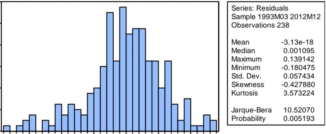
5.3.4 Normality Test

This test is important to find out whether the error term follows normal distribution and the hypotheses are stated as follows:

(29)

29

Residuals are normally distributed Residuals are not normally distributed

Figure 3 shows the Eviews output. The histogram shows that residuals are not normally distributed. The non-normality of residuals is also confirmed by the Jarque-Bera test since the p-value (0, 005193) is smaller than the critical p-value at the 5% level. So, the null hypothesis can be rejected, thus residuals are not normally distributed. The non-normal behavior observed can be explained by the fact that consumer price index increases continuously during the period of examination (appendix Figure 5a) compared to the other variables where we can observe some upward or downward movements over the 20-year time span.

Although the residuals are non-normally distributed, we can rely on our t-tests results since we use a reasonably large sample in our linear regression.

Figure 3: Histogram of residuals and Jarque-Bera test

From our diagnostic checking results, we can assume that residuals from our linear regression are white noise, meaning that they do not contain any systematic information. However, in reality it is hard to find a model with completely white noise residuals; this is confirmed by the normality test where we found that residuals are not normally distributed.

5.3.5 Granger Causality Test

The Granger Causality test is a statistical hypothesis test to determine whether one time series is significant in forecasting another. This test aims at determining whether past values of a variable help to predict changes in another variable (Granger, 1988). In addition, it also says that variable

0 4 8 12 16 20 24 -0.15 -0.10 -0.05 0.00 0.05 0.10 Series: Residuals Sample 1993M03 2012M12 Observations 238 Mean -3.13e-18 Median 0.001095 Maximum 0.139142 Minimum -0.180475 Std. Dev. 0.057434 Skewness -0.427880 Kurtosis 3.573224 Jarque-Bera 10.52070 Probability 0.005193

(30)

30

Y is Granger caused by variable X if variable X assists in predicting the value of variable Y (Sarbapriya, 2012).

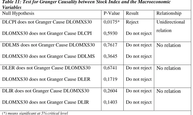
In our empirical research, the Granger Causality test is conducted to study the causal relationship between the macroeconomic variables and the Stockholm Stock Exchange. By applying the ADF test, the first difference of four variables and second difference MS is performed to obtain stationary variables before using them on Granger causality test. Table 11 below reports the Granger causality test results with a lag of 4 as the lag selection.

We can conclude that there is a unidirectional relationship between inflation rate (CPI) and stock price since we reject the null hypothesis that DLCPI does not Granger Cause DLOMXS30; the p-value (1,75%) is less that the critical value (5%). This means that that inflation Granger causes stock price.

The overall Granger Causality test reveals that only inflation granger causes the stock prices while the stock prices do not affect any of the four macroeconomic variables included in the research.

Table 11: Test for Granger Causality between Stock Index and the Macroeconomic Variables

Null Hypothesis P-Value Result Relationship

DLCPI does not Granger Cause DLOMXS30 DLOMXS30 does not Granger Cause DLCPI

0,0175* 0,5930 Reject Do not reject Unidirectional relation DDLMS does not Granger Cause DLOMXS30

DLOMXS30 does not Granger Cause DDLMS

0,7617 0,3645

Do not reject

No relation

DLER does not Granger Cause DLOMXS30 DLOMXS30 does not Granger Cause DLER

0,6741 0,1719

Do not reject

Do not reject No relation

DLIR does not Granger Cause DLOMXS30 DLOMXS30 does not Granger Cause DLIR

0,2604 0,1403

Do not reject Do not reject

No relation

(31)

31

6 Discussion and Conclusion

The role of the stock market in the economy is to raise capital and also to ensure that the funds raised are utilized in the most profitable opportunities. This empirical report performs the necessary analysis to answer whether changes in the identified macroeconomic variables affect stock prices of the Stockholm Stock Exchange. The research employs regression analysis and Granger causality test to examine these relationships. The linear regression test results show that high inflation and Swedish krona depreciation against the Euro are negatively and significantly related to the stock prices of the Stockholm Stock Exchange (OMXS30). Besides inflation and exchange rate, there is also a negative but insignificant relationship between interest rate and stock price.

The negative relationship between inflation and stock price can be explained by the fact that additional funds flow due to inflation increase the supply in the stock market while the demand side remains unaffected. This static condition on the demand side of the security market puts downward pressure on the stock price. It is important for investors to follow the CPI because periods of high inflation make difficult the market conditions. Besides, deprecation of Swedish krona (exchange rate) and high interest rate decrease the flow of capital and this will also decrease the additional funds flowing in the stock market. On the other hand, a positive relationship is found between stock price and money supply although it is insignificant. Furthermore, the Granger causality test shows that inflation is the only macroeconomic variable that causes stock price while stock price has no effect on any of the macroeconomic variables.

On the basis of the above overall analysis, it can be concluded that two out of the four selected macroeconomic variables are relatively significant and likely to influence the stock prices of the Stockholm Stock Exchange. These macroeconomic variables are inflation and exchange rate. The evidence of this study is consistent with other similar studies. However, the results from this empirical research should not be a conclusive indicator for investment.

6.1 Further Research

Besides macroeconomic conditions, there are many other factors that affect the prices of stocks and its movements. A host of such factors are found in the microeconomic variables. The idea is

(32)

32

that the performance of particular companies and their results matter in determining the price of a stock. Indeed, high corporate profits lead to higher stock prices due to high demand. Moreover rumors of positive news for firms and the re-purchase of shares listed give a positive impact and lead to higher stock prices. Thus for further study, we could discuss the role of micro economic factors on stock price and how an investor can reduce microeconomic risk by undertaking a strong portfolio diversification strategy

(33)

33

7 References

Abeyratna G., Anirut P., and David M. P. (2004) “Macro-economic Influences on the Stock Market Evidence from an Emerging Market in South Asia” Journal of Emerging Market

Finance, December 2004,, Vol. 3, no. 3, 285-304.

Ajayi R.A. and Mougoue M. (1996) “On the Dynamic Relation between Stock Prices and Exchange rates” The Journal of Financial Research 19, 193-207.

Avneet K. A., Chandni M., and Saakshi C. (2012) “A Study of the effect of Macroeconomic Variables on Stock Market: Indian Perspective”. Electronic copy available at: http://ssrn.com/abstract=2178481.

Bahmani-Oskooee M., and Sohrabian A. (1992) “Stock prices and the effective exchange rate of the dollar” Applied Economics, 24 (4): 459-64.

Bhattacharya B, Mookherjee J (2001), Causal relationship between and exchange rate, foreign exchange reserves, value of trade balance and stock market: case study of India. Department of

Economics, Jadavpur University, Kolkata, India.

Barro R. J. (1990) “The Stock Market and Investment” Review of Financial Studies 3, 115–131.

Barro R. J. (1974) “Are Government Bonds Net Worth?” Journal of Political Economy 82, pp. 1095-1117.

Blanchard O.J. (1987) “Vector Autoregressions and Reality: Comment” Journal of Business and

Economic Statistics, 1987, Vol. 5, No. 4, pp. 449-451.

Chen, N. F., Richard Roll and Stephen A. Ross (1986) “Economic Forces and the Stock Market”,

Journal of Business, 59, pp. 383-403.

Choi D., and Jen F. (1991) “The relation Between Stock Returns and Short-Term Interest Rates”

Review of Quantitative Finance and Accounting, 1991, Vol. 1, pp. 75-89.

Connor G., and Korajczyk A. R. (1993) “The Arbitrage Pricing Theory and Multifactor Models of Asset Returns” Working paper # 139.

(34)

34

Conover M. C., Jensen G. R., and Johnson R. R. (1998) “Monetary Environments and International Stock Returns”, Journal of Banking and Finance, 1999, Vol. 23, pp. 1357-1381.

Cooper, R.V. (1974) “Efficient Capital Markets and the Quantity Theory of Money”, Journal of

Finance, 24, pp. 887-921.

Darat, A.F. and Mukherjee T. K. (1987) “The Behaviour of a Stock Market in a Developing Economy”, Economic Letters, 22, 273-278.

Darrat, A. F. (1990a). “Stock Returns, Money and Fiscal Deficits”, Journal of Financial and

Quantitative Analysis 25, 387-398.

Dhakal, D., M. Kandil, and S. C. Sharma (1993) “Causality between the Money Supply and Share Prices: A VAR Investigation” Quarterly Journal of Business and Economics 32, 52–74. Dickey, D.A, Fuller, W.A. (1979) “Distributions of the Estimators for Autoregressive Time Series with a Unit Root”, Journal of American Statistical Association 74:366, pp. 427-481. Doong, S.-Ch., Yang, Sh.-Y., Wang, A., (2005) “The dynamic relationship and pricing of stocks and exchange rates: Empirical evidence from Asian emerging markets,” Journal of American

Academy of Business, Cambridge, Vol.7, No1, pp.118-23.

Elton, J. E., Gruber, M. J., Brown, S. J. and Goetzmann, W. N., (2010) “Modern Portfolio Theory

and Investment Analysis”, 8th International student edition, John Wiley & Sons.

Fama, E. (1970) “Efficient Capital Markets: A Review of Theory and Empirical Work” The

Journal of Finance, Vol. 25, No. 2, pp. 383-417.

Fama, E.F. (1981) “Stock returns, real Activity, Inflation, and Money”, The American Economic

Review, 71(4), 545-565.

Fama, E., F, (1990) “Stock returns, expected returns, and real activity”, The Journal of Finance 45, 1089-1108.

Fama, E. F. and K. R. French (1989) “Business Conditions and Expected Returns on Stocks and Bonds”, The Journal of Financial Economics 25, 23–49.

(35)

35

Fama, E.F. and Schwert, W., (1977), “Asset returns and inflation”, Journal of Financial

Economics, Vol. 5, pp. 115-46.

Firth, M., (1979), “The relationship between stock market returns and rates of inflation”, Journal

of Finance, Vol. 34, 743-49.

Geetha C., Mohidin R., Chandran V. V., and Chong V. (2011) “The Relationship between Inflation and Stock Market: Evidence from Malaysia, United States and China”. International

Journal of Economics and Management Sciences, Vol. 1, No. 2, 2011, pp. 01-16.

Gjerdr, Oystein and Frode Saettem (1999), “Causal Relation among Stock Returns and Macroeconomic Variables in a Small, Open Economy”, Journal of International Financial

markets, Institutions and Money, Vol. 9, pp. 61-74.

Gujrati, D.N. and D.C. Porter (2009) Basic Econometrics, Fifth Edition, McGraw Hill, USA.

Granger, C. W. J. (1981), “Some properties of Time Series Data and their use in Econometric Model Specification”, Journal of Econometrics, Annals of Applied Econometrics, 16: 121-30.

Granger, C.W.J (1986), “Developments in the Study of Cointegrated Economic Variables”,

Oxford Bulletin of Economics and Statistics, nr. 48.

Grossman, S.J and Shiller R.J. (1981) “The Determinants of the Variability of Stock Market Prices”, The American Review 1981, Vol. 71, No. 2, pp. 222-227.

Hamburger Michael J. and Levis A. Kochin (1971) “Money and Stock Prices: The Channels of Influences”, The Journal of Finance, 27(2): 231-249.

Homa, Kenneth E. and Dwight M. Jaffee. 1971. “The Supply of Money and Common Stock Prices”, Journal of Finance, 26(5): 1045-1066.

Jaffe, J.F. and Mandelker, G., (1977) “The ‘Fisher Effect’ for risky assets: An empirical investigation”, Journal of Finance, Vol. 32, 447-58.

Jensen G. R., Mercer J. M., Johnson R. R. (1995) ”Business Conditions, Monetary Policy, and Expected Security Returns”, Journal of Financial Economics, 1996, Vol. 40, pp. 213-237.

(36)

36

Lintner, J., (1973), “Inflation and common stock prices in a cyclical context”, National Bureau of

Economic Research Annual Report.

Mahedi Masuduzzaman (2012) “Impact of the Macroeconomic Variables on the Stock Market Returns: The Case of Germany and the United Kingdom”, Global Journal of Management and

Business Research.

Mohammad, B.A. (2011) “Impact of Micro and Macroeconomic Variables on Emerging Stock Market Return: A Case on Dhaka Stock Exchange (DSE)”, Interdisciplinary Journal of Research

in Business.

Roll, Richard (1977) “A critique of the asset pricing theory's tests”, Journal of Financial

Economics, March 1977, p. 129.

Roll, Richard and Stephen Ross (1980) “An empirical investigation of the arbitrage pricing theory”, Journal of Finance, Dec 1980, p. 1073.

Roll, Richard and Stephen Ross (1984) “The Arbitrage Pricing Theory Approach to Strategic Portfolio Planning”, Financial Analysts Journal, Vol. 40, No. 3 (May-June 1984), pp. 14-99 + 22-26.

Sellin, Peter (2001) “Monetary Policy and the Stock Market: Theory and Empirical Evidence.”,

Journal of Economic Surveys, 2001, 15 (4), pp. 491-541.

Sarbapriya, Ray (2012) “Foreign Exchange Reserve and its Impact on Stock Market Capitalization: Evidence from India”, Research on Humanities and Social Sciences, Vol.2, No.2, 2012.

Uddin, M. G. S. and Alam, M. M. (2007) “The Impacts of Interest Rate on Stock Market: Empirical Evidence from Dhaka Stock Exchange”, South Asian Journal of Management and

(37)

37

8 Appendix

8.1 Appendix 1: ADF Test

8.1.1 Stock Price (OMXS30)

Figure 4a: Data graph set at level Figure 4b: Data graph set at first difference

Table 12a: Unit Root test at level

Null Hypothesis: LOMXS30 has a unit root Exogenous: Constant, Linear Trend

Lag Length: 0 (Automatic - based on SIC, maxlag=14)

t-Statistic Prob.*

Augmented Dickey-Fuller test statistic -2.338122 0.4113

Test critical values: 1% level -3.996918

5% level -3.428739

10% level -3.137804

*MacKinnon (1996) one-sided p-values.

Augmented Dickey-Fuller Test Equation Dependent Variable: D(LOMXS30) Method: Least Squares

Date: 05/08/13 Time: 15:06

Sample (adjusted): 1993M02 2012M12 Included observations: 239 after adjustments

LOMXS30(-1) -0.028889 0.012356 -2.338122 0.0202

C 0.188962 0.073084 2.585527 0.0103

@TREND(1993M01) 6.18E-05 8.80E-05 0.702575 0.4830

Adjusted R-squared 0.025429 S.D. dependent var 0.061724 S.E. of regression 0.060934 Akaike info criterion -2.745581

4.8 5.2 5.6 6.0 6.4 6.8 7.2 7.6 1994 1996 1998 2000 2002 2004 2006 2008 2010 2012 LOMXS30 -.20 -.15 -.10 -.05 .00 .05 .10 .15 .20 1994 1996 1998 2000 2002 2004 2006 2008 2010 2012 DLOMXS30

(38)

38

Table 12b: Unit Root test at First Difference

Null Hypothesis: DLOMXS30 has a unit root Exogenous: Constant

t-Statistic Prob.*

5% level -2.873492

10% level -2.573215

Augmented Dickey-Fuller Test Equation Dependent Variable: D(DLOMXS30) Method: Least Squares

Date: 05/08/13 Time: 15:06

DLOMXS30(-1) -0.915322 0.064499 -14.19131 0.0000

C 0.006658 0.004012 1.659553 0.0983

R-squared 0.460440 Mean dependent var -0.000382

(39)

39

8.1.2 Consumer Price Index (CPI)

Figure 5a: Data graph set at Level Figure 5b: Data graph set at first difference

Table 13a: Unit Root test at level

Null Hypothesis: LCPI has a unit root Exogenous: Constant, Linear Trend

t-Statistic Prob.*

5% level -3.429745

10% level -3.138397

Augmented Dickey-Fuller Test Equation Dependent Variable: D(LCPI)

Method: Least Squares Date: 05/08/13 Time: 15:05

LCPI(-1) -0.062361 0.018453 -3.379350 0.0009 D(LCPI(-1)) 0.076480 0.061712 1.239306 0.2166 D(LCPI(-2)) -0.003993 0.062184 -0.064218 0.9489 D(LCPI(-3)) 0.060000 0.061247 0.979641 0.3284 D(LCPI(-4)) -0.041234 0.061320 -0.672441 0.5020 D(LCPI(-5)) 0.098577 0.059815 1.648046 0.1008 D(LCPI(-6)) 0.174093 0.060284 2.887886 0.0043 D(LCPI(-7)) 0.097530 0.061132 1.595390 0.1121 D(LCPI(-8)) -0.100681 0.061567 -1.635314 0.1035 D(LCPI(-9)) 0.008292 0.061434 0.134974 0.8928 D(LCPI(-10)) -0.065693 0.061549 -1.067324 0.2870 D(LCPI(-11)) 0.021451 0.061714 0.347587 0.7285 D(LCPI(-12)) 0.453105 0.062955 7.197310 0.0000 5.48 5.52 5.56 5.60 5.64 5.68 5.72 5.76 1994 1996 1998 2000 2002 2004 2006 2008 2010 2012 LCPI -.015 -.010 -.005 .000 .005 .010 .015 1994 1996 1998 2000 2002 2004 2006 2008 2010 2012 DLCPI

(40)

40

C 0.342300 0.101116 3.385223 0.0008

@TREND(1993M01) 6.78E-05 2.02E-05 3.357009 0.0009

Table 13b: Unit root test at first difference

Null Hypothesis: DLCPI has a unit root Exogenous: Constant

t-Statistic Prob.*

5% level -2.874143

10% level -2.573563

Augmented Dickey-Fuller Test Equation Dependent Variable: D(DLCPI)

DLCPI(-1) -0.723163 0.215339 -3.358253 0.0009 D(DLCPI(-1)) -0.165876 0.213223 -0.777947 0.4375 D(DLCPI(-2)) -0.202589 0.202566 -1.000116 0.3184 D(DLCPI(-3)) -0.192171 0.191045 -1.005894 0.3156 D(DLCPI(-4)) -0.266742 0.181621 -1.468670 0.1434 D(DLCPI(-5)) -0.212837 0.173083 -1.229685 0.2202 D(DLCPI(-6)) -0.053967 0.166606 -0.323918 0.7463 D(DLCPI(-7)) 0.025794 0.157323 0.163957 0.8699 D(DLCPI(-8)) -0.108493 0.143267 -0.757281 0.4497 D(DLCPI(-9)) -0.149503 0.125576 -1.190544 0.2352 D(DLCPI(-10)) -0.248080 0.108681 -2.282651 0.0234 D(DLCPI(-11)) -0.263714 0.089662 -2.941199 0.0036 D(DLCPI(-12)) 0.168842 0.069071 2.444470 0.0153 C 0.000767 0.000319 2.406206 0.0170

R-squared 0.675635 Mean dependent var -3.29E-06

(41)

41

8.1.3 Money Supply (MS)

Figure 6a: Data graph set at level Figure 6b: Data graph set at first difference

Figure 6c: Data graph set at second difference

Table 14a: Unit root test at level

Null Hypothesis: LMS has a unit root Exogenous: Constant, Linear Trend

t-Statistic Prob.*

Augmented Dickey-Fuller test statistic 1.153678 0.9999

5% level -3.429745

10% level -3.138397

Augmented Dickey-Fuller Test Equation Dependent Variable: D(LMS)

10.9 11.0 11.1 11.2 11.3 11.4 11.5 11.6 1994 1996 1998 2000 2002 2004 2006 2008 2010 2012 LMS -.08 -.04 .00 .04 .08 .12 1994 1996 1998 2000 2002 2004 2006 2008 2010 2012 DLMS -.20 -.15 -.10 -.05 .00 .05 .10 1994 1996 1998 2000 2002 2004 2006 2008 2010 2012 DDLMS