FROM STRUCTURAL EQUATION MODELING TO MACROSCOPIC
FUNDAMENTAL DIAGRAMS: INVESTIGATING THE IMPACT OF
ROAD SEGMENTS SAFETY ON NETWORK LEVEL EFFICIENCY
Justin P. Schorr
The George Washington University Science and Engineering Hall, Room 3810 800 22nd Street, NW, Washington, DC 20052
Phone: +1-202-994-6652 E-mail: justin11@gwmail.gwu.edu
Co-authors(s); Samer H. Hamdar, The George Washington University; Seungmo Kang, Korea University; Kitae Jang, Korea Advanced Institute of Science and Technology; Hussein Kachouch, American University of Beirut
ABSTRACT
The main objective of this research is to expand upon the link between network flow (mobility) and safety through the estimation of Macroscopic Fundamental Diagrams (MFD) and Structural Equation Models (SEM) with different levels of disruptions caused by different surrounding driving conditions. Analysis begins with the aggregation of microscopic level loop detector data and collision data provided by The Korea Expressway Corporation (KEC). The KEC operates highway tolls throughout South Korea and continues to expand upon the nearly 4000 km of high-speed motorways it provides. The rich, detailed collision and traffic flow data collected on these roadways makes the region an ideal candidate for the new analysis technique that is presented in this study. Three specific types of non-recurrent disruptions, as suggested by SEM results, (inclement weather conditions; increased holiday demand; increased number of collisions) are analyzed and compared in this study. By estimating and comparing MFDs for these specific cases, the differences in network level disruptions caused by these events are visualized, quantified and discussed. Additionally, by using SEM to quantify the impact of these disruptive events on safety and impedance at the link level, spatial and temporal analysis can be conducted – establishing a link between the microscopic event-based data (mainly collisions) and the macroscopic network performance measures of safety and traffic mobility.
1.
INTRODUCTION AND OBJECTIVES
Modernization of transportation systems and infrastructure is a major initiative championed by individual countries throughout the global community. South Korea is no exception as there is constant updating of infrastructure from highways, railways and public transport systems (Ro, 2002). The Korea Highway Corporation operates highway tolls and provides over 1800 miles of both high speed motorways and national highways (KEC, 2015). Cities have intercity and intracity bus services providing efficient mobility to the public, as well as an expanding high speed rail and subway networks from technological progress.
Despite the country’s high quality of roadways and infrastructure, South Korea’s traffic fatality rate is 14.1 per 100,000 people ranking it 104th worldwide with an average 6,784 casualties per year (WHO,
2015). While the number of collisions (from 290,938 to 223,656), fatalities (from 10,236 to 5,392) and injuries (from 426,984 to 344,565) have all decreased from 2002 to 2012, South Korea’s traffic related fatality rate still ranks it 30th out of the 31 countries that comprise the Organization for Economic
Cooperation and Development (OECD) (YNA, 2014). Traffic conditions can be summarized as very congested due to the rapid increase of vehicles and licensed drivers in the country (Park, 2008) where a majority of the congestion concentrates in Seoul along the Namsan Tunnel 1 and Namsan Tunnel 3 (AngloINFO Seoul, 2015). Enforcing congestion charges however for non-carpooling vehicles in the Namsan Tunnels has shown significant drops in traffic volumes during the time the charge is applied (12% increase before the charge time and 20% increase after the charge time) (Bae, 2013).
Linking network flow (mobility) and safety, traffic management and control measures are often applied to regulate congestion levels while maintaining the safety of users in the system (RGB Spectrum, 2008). Proper application of these measures requires knowledge of potential impacts on individual network links as well as the entire system’s average flow and density. One approach to look into the system’s flows and densities, as an aggregate outcome of individual links’ performance, is through the use of macroscopic fundamental diagrams (MFDs). Estimation of network level macroscopic flow diagrams (MFD) is, however, challenging as ideal traffic flow conditions are not universally observed on all links throughout the entire network (Mohan & Ramadurai, 2013). Thus, a statistical model can be estimated prior to building the MFDs such as to provide a basis for data selection and results interpretation. For this study a structural equation model (SEM) is introduced as this type of model allows for a dimentional grouping or variables that can be used both in the selection of data for MFD estimation and in the interpretation of said estimations.
In other words, the main objective of this paper is to further expand on the link between network flow (mobility) and safety through the estimation of macroscopic fundamental diagrams and structural equation models. In both estimations, consideration will be given to the intertwining relationship of safety and flow. Specifically, the tasks to be realized in this study are as follows:
Estimate a structural equation model using collision data provided by the KEC
Based on the achieved SEM, select specific days that correspond to the associated dimentional groupings
Estimate MFDs for the selected days
Analyze the achieved MFDs both on their own and within the context of the achieved SEM In line of the aforementioned tasks, Section 2 offers a brief background related to the macroscopic fundamental diagram (MFD) and its use to understand network level traffic phenomena. Using data from the Korean Highway Network, Section 3 presents the structural equation model that classifies the types of disruptions impacting the safety and the mobility performance of the different roadway links
studied in this paper. Such classification motivates the data mining and modification used in Section 4 to estimate the MFDs during different times of the year. The numerical results are then presented and analyzed in Section 5 before concluding with some future research needs.
1.1. Background and Motivation
Fundamental Diagrams of traffic flow are the cornerstone of traffic flow theory, but until recently they have been estimated for specific links (microscopic level). On the microscopic level, speed, flow and density characteristics can be measured for each link within the transportation network by collecting data from field tests. Field tests can be achieved where observers perform vehicular counts or observe the time interval it needs for vehicles to traverse a certain distance on a roadway segment (Mathew & Rao, 2006; Jia et al., 2014). Collecting the raw data from the field allows the data to be aggregated for concluding relations on how microscopic traffic flow behaves. From a macroscopic perspective, roadway links operate in a conjoined manner, meaning that link specific characteristics impact and are impacted by those of the other links throughout the entire transportation network. Daganzo (2007) and expanded this application, suggesting that networks facing homogeneous conditions will operate under a Macroscopic Fundamental Diagram (MFD) that relates the production to the accumulation, and can also correlate traffic production with the rate at which vehicles enter and leave a network. By obtaining such a relationship, the author suggests the possibility of predicting future traffic conditions based on the functionality of the entire network from a fixed generalization that can be obtained from further testing and research.
A significant amount of recent studies have focused on the estimation of MFDs, as well as the challenges and breakdowns that require attention. Modeling traffic in large urban regions using aggregated outputs from pre-timed traffic signals can allow the estimation of the average MFD (Daganzo & Geroliminis, 2008). Simulating networks can also reproduce MFDs by defining origin-destination (O-D) zones and deriving the macroscopic model from the microscopic one (Ji et al., 2010). MFDs have also been more accurately approximated by collecting raw data through simulation tools and combining it with vehicle trajectory data retrieved from probes and loop detectors (Leclercq et al., 2014).
Collecting and analyzing data from a region under study may suggest the existence of an MFD, but it does not necessarily prove this existence; often due to disruptions in homogeneous traffic conditions which are considered ideal for estimation purposes (other challenges for estimation include weather, geometric and collision based disruptions of ideal traffic conditions) (Geroliminis & Daganzo, 2008; Geroliminis & Sun, 2011; Wang et al., 2015; Geroliminis et al., 2014). Traffic conditions become homogeneous when considering lengthy straight roadways with specific widths due to the constant driving patterns that different drivers endure (Daganzo & Geroliminis, 2008). Environmental surroundings also contribute to MFD behavior where poorer weather and lighting conditions cause the formation of a hysteresis loop in the diagram as opposed to clear weather settings (Ji et al., 2010). Moreover, collisions have found to create bottlenecks on arterials which produced flow disruptions and heterogeneous traffic conditions that caused hysteresis loop formations in the MFD (Ji et al., 2010; Geroliminis et al., 2014).
Corrections for heterogeneity have been applied by various authors to produce an approximate estimate of the MFD in the region under study (Daganzo & Geroliminis, 2008; Leclercq et al., 2014; Knoop et al., 2013). MFD plots showed disordered scattering upon congestion which had to be accounted for by further testing and better traffic signalization for minimizing errors produced due to heterogeneity (Daganzo & Geroliminis, 2008). GPS equipped taxis that would conduct trips in the network would also help better approximate estimated MFDs from loop detectors which would
account for the generated errors (Geroliminis & Daganzo, 2008). As other studies also showed, disordered traffic conditions would generally cause overestimations in the MFDs (Leclercq et al., 2014, Knoop et al., 2013). Critical density values would cause enlargements in MFD flow which would result in inadequate approximations deviating from the real value which would need adjustments by more accurate simulations (Knoop et al., 2013).
Given the aforementioned challenges estimating MFDs when traffic disruptions and heterogeneity (in link characteristics) are encountered, this paper utilizes structural equation modeling to study traffic safety issues and disruptions. Such safety issues (represented by roadway collisions) and disruptions (associated with inclement weather conditions and high demand) encountered on the Korean Highway Network are then linked to different MFDs estimated during different times of the year.
2.
STRUCTURAL EQUATION MODELLING
Collision data provided by the KEC featured 29,873 individual collisions occurring between 2011 and 2013. The initial dataset had 79 descriptive variables for each collision, and a guide to the variables used for analysis as well as how they were coded is provided in Appendix A. After filtering out data with missing variables, the set used for analysis consisted of 14,286 complete collision records (3584 from 2011; 4845 from 2012; 5857 from 2013) and 56 descriptive variables.
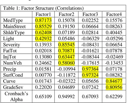
Formulation of the SEM model follows that of Hamdar et al. (2008) – which begins by conducting a factor analysis and ends with the estimation of an SEM. For this study, the proposed endogenous variables all related to the disruption in traffic caused by the collision (total closed time, total turnaround time, time to first arrival, total traffic blocking time). Continuing, a factor analysis was conducted based on the following proposed exogenous dimensions: L1 – Driver Related Characteristics (speed, gender, age, driver condition), L2 – Collision Related Characteristics (severity, number of injuries, number of fatalities, number of vehicles) L3 – Weather Related Characteristics (precipitation, surface condition, lighting), and L4 – Infrastructure Related Characteristics (curve, grade, median type, shoulder type, location of collision). After multiple estimations it was clear that the driver characteristics’ dimension needed to be dropped from the model due to consistently low factor scores. Furthermore, the remaining variables and their associated scores (after the removal of the driver characteristics) suggested new dimensional groupings. The rotated factor structure based on the remaining variables is as follows:
Table 1: Factor Structure (Correlations)
Factor1 Factor2 Factor3 Factor4 MedType 0.87173 0.15078 0.02252 0.15576 MainStreet 0.85529 0.19150 0.06664 0.08263 ShldrType 0.62408 0.07189 0.02814 0.40445 Light 0.42932 0.05486 -0.06329 -0.05296 Severity 0.13933 0.85545 -0.08431 0.06654 FatTot 0.02018 0.70871 -0.01621 0.07878 InjTot 0.13080 0.63447 -0.08344 -0.02469 NumVeh 0.24662 0.58060 -0.17615 -0.13453 Precip 0.01581 -0.10994 0.97364 0.07178 SurfCond 0.00770 -0.11872 0.97324 0.08282 Curve 0.01743 -0.02322 0.05656 0.84677 GradeSev 0.22020 0.04689 0.07242 0.80956 Cronbach’s Alpha 0.65109 0.94992 0.67093 0.62299
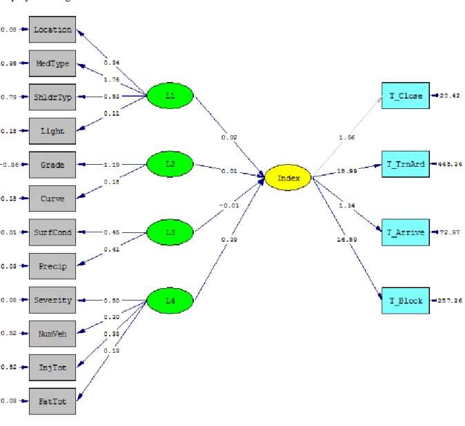
Factor scores on the order of 0.1 were considered for analysis (Hamdar et al., 2008). The achieved factor structure suggested the following dimensions which were used to estimate the SEM: L1 – Traffic Related Characteristics (location of collision, median type, shoulder type, lighting), L2 – Collision Related Characteristics (severity, number of injuries, number of fatalities, number of vehicles) L3 – Weather Related Characteristics (precipitation, surface condition), and L4 – Infrastructure Related Characteristics (curve, grade). In an attempt to confirm the results of the factor analysis and check the internal consistency of the model, Cronbach’s alpha was utilized (Cortina 1993). The cutoff for statistical significance is 0.7 (Sijtsma 1999), a threshold that is nearly reached by the L1, L3, and L4 dimensions and is exceeded by the L2 dimension – indicating that the model is sufficiently stable as suggested by Sijtsma (2009) (alpha is typically calculated when variables are either dichotomous or have the same scale and even then only assesses the degree to which variables are inter-related. Several structures were then tested based on these new dimensions ultimately leading to the statistically significant converging model (computed using the LISREL software) displayed in Figure 1.
Figure 1: Structural Equation Model
As suggested by Golob (2001), in models with large sample sizes (such as this, N=14286) chi-squared tests often encounter problems; thus the goodness of fit was assessed based on the root mean square
error of approximation (RMSEA) (Golob 2001). For the model above, the RMSEA was 0.051 and the 90% confidence interval was 0.050; 0.052. The entire confidence interval is around the threshold of 0.05 indicating that the model is statistically significant and has a good fit (Golob 2001; Hu and Benlter 1998). For further support, the standardized root mean square residual (SRMR) has a value of 0.039; values less than 0.08 are generally considered to indicate a good fit (Hu and Bentler 1998). Additional fit statistics such as the Goodness of Fit Index (GFI = 0.97) and Adjusted Goodness of Fit Index (AGFI = 0.96) indicated that the model was statistically significant as well. Lastly, for an alpha of 0.05, t-values greater than1.96 or less than -1.96 are considered significant – a threshold at which only two paths marginally did not achieve (L2 to INDEX: t-value of 1.53; L3 to INDEX: t-value of -0.91). T-values indicate that we can be more confident in some paths than others, and all t-values in the model were either significant or on the close to being so.
The impact of exogenous variables on the endogenous time related variables is interpreted based on two main values – the coefficient of variation and the contribution to the index from a one standard deviation change in the variable. Using these two measures speaks to both how much the variable is changing throughout the dataset (coefficient of variation) and the impact that those changes have on the time-related INDEX (deviation contribution). The most influential variables in the model come from the L4 dimension (Collision Related Characteristics), led by injury total and fatality total – an expected result as major collisions with multiple injuries and fatalities are likely to require more time to clear them from the roadway. Other notable results from the SEM estimation are: in terms of the Infrastructure Related Characteristics (L2), roadway curvature has a larger impact on the INDEX than grade; and for the Traffic Related Characteristics, median type and location have less of an impact on the INDEX than shoulder type and lighting. Finally, the only counterintuitive results in the model come from the L3 dimension (Weather Related Characteristics) where both surface condition and precipitation are indicative of a reduction in the time related variables. While this result may be due to an overabundance of non-weather related collision in the dataset, it may also be due to a reduction in traffic demand on days with heavy precipitation – allowing for faster response and ultimately a reduction in the time the vehicles remain on the roadway. This result, along with the other results from the SEM estimation, will be discussed in further detail after the MFDs are estimated.
Based on the achieved structural model, it is clear that additional consideration needs to be given to the disruptions caused collisions (expressed by the endogenous variables presented in Figure 1) and their relation to high demand and weather conditions (possibly clarifying the counterintuitive result discussed above). Thus the selection of the days for which MFD estimation will be conducted is done based on the achieved SEM, and will include multiple days featuring different high collision rates, different precipitation levels and different demand levels.
3.
MFD ESTIMATION
As proposed by Daganzo, MFDs relate the average production (flow) with the average accumulation (density) in the network (Daganzo, 2007). Since each highway segment consists of different flows, densities and lengths, the weighted average must be computed. First, given the flow and length of individual roadway segments, the average weighted flow at a given time t is:
𝑞𝑎𝑣𝑔,𝑡 = ∑ 𝑞𝑖,𝑡𝐿𝑖 𝑖
∑ 𝐿𝑖 𝑖
⁄ Equation 1
Where: qavg is the average weighted flow in vehicles per 5 minutes per lane (v/5min/l); qi is the flow
rate of each roadway segment in vehicles per 5 minutes per lane (v/5min/l), and Li is the roadway
𝑘𝑎𝑣𝑔,𝑡 = ∑ 𝑘𝑖,𝑡𝐿𝑖 𝑖
∑ 𝐿𝑖 𝑖
⁄ Equation 2
Where: kavg is the average weighted density in vehicles per kilometers per lane (v/k/l); ki is the density
of each roadway segment in vehicles per kilometer/lane (v/k/l); and Li is the roadway length under
consideration in kilometers (km). By obtaining the average flow and density, values are aggregated to construct the flow-density relationships for the roadway network. Thus, the fundamental behavior of the three diagrams (flows vs. density, speed vs. density, and speed vs. flow) can be deduced. Upon deducing these relationships, the models can be compared to one another for potential similarities between them and possible MFD behavior governing the network.
3.1. Data Description
The dataset used for analysis featured loop detector data for the majority of the South Korean highway network for seven specific days in 2013. These days were selected based on the achieved structural model as to best capture the differences in the three non-recurrent disruptions (weather related, congestion/demand related and collision related). The four days with the most collisions in 2013 were selected (two weekdays: February 4th – 90 collisions, no precipitation and November 27th - 87
Collisions, light precipitation; two weekend days: September 29th – 71 collisions, moderate
precipitation and September 14th – 70 collisions, light precipitation). Additionally, the two days with
the most precipitation were selected (October 8th – rain, 61 collisions and December 14th – snow, 28
collisions) as well as a day during the Chuseok holiday (September 19th – which features an increase in
congestion throughout the network, as well as 20 collisions and no precipitation).
The most challenging aspect of the data set are the troubles that are inherent to dealing with over 30 million lines of data. Complicating matters, three datasets needed to be combined in order to aggregate all data needed for analysis. In the first two files, speed and volume, data is coded as follows: date, time interval, transponders (detector id), lane number (if there are three lanes, this would correspond to three lines of data for the same detector id), and either the speed or volume. The third file was organized based on detector id, post-kilometer, longitude, and latitude. Only complete records were used for analysis – that is only detectors that contained both speed and volume data at a given time, as well as only those that could be located based on their geographic coordinates.
Further complications arise when considering the manner in which the detector identification numbers were coded. An example detector id is as follows: “0010VDE00100”, where the first four numbers “0010” correspond to the link number, the next three “VDE” correspond to the direction (East in this case, South is coded as “VDS”), and the final five characters “00100” correspond to the detector id within the corresponding link (“0010”). Using the geographic locations of the detectors, manual inspection of the dataset revealed a number of issues with the identification numbers. Figure 2 shows the first of these problems.
Figure 2: Example of a Discontinuous Link
Here, the link “0120” is coded as a singular link based on the associated identification number, but as the figure shows – this is clearly not the case. Not only is this link discontinuous over a large geographic area, but the beginning portion of the link (left side of the figure) crosses over another major link in the highway network. As such, manual inspection of all links was conducted using the ArcGIS software such that they could be separated into segments. Segments were divided in a logical, consistent and organized fashion based first on the intersection with other links in the network, and then by restricting the maximum segment length to approximately 10 kilometers (aggregation was conducted at both levels). Another illustrative example of this separation process is provided for link “0100” in Figures 3A and 3B below.
Figures 3A and 3B: Link Segmentation Example (left) and Transponder Identification Example (right)
As mentioned above, each segment created along the link in consideration constitutes a section of uninterrupted flow along the link (i.e. no major highways or arterials intersect the individual segments). Manually choosing the starting and ending transponders of the created segment allowed for the required analysis variables to be aggregated and defined appropriately (Figure 3B). In addition to separating the links into segments, manual inspection of all links helped in:
1. Verifying that sequentially numbered detectors were part of the same segment (which was not the case for all detectors). To combat this, segments were defined such that the detectors were assigned to the correct segment and placed in the correct order.
2. Identifying instances where detectors occupied the same postmile, which occured when on and off ramps featured detectors. These detectors were dropped from the dataset as they often featured values of 0 or -1, and were generally troublesome in the estimation process.
3. Identifying an overabundance of instances where detectors were zero-valued. While many of these instances certainly corresponded to unoccupied lengths of roadway – manual inspection demonstrated that a large amount corresponded to malfunctioning detectors. These detectors were dropped from the dataset – with the exception of instances where more than four consecutive detectors were zero-valued.
Although tedious, was certainly necessary in order to minimize and aggregation error as much as possible. The level of aggregation has a definite impact on the resulting MFD and should be given due consideration in the estimation process.
4.
RESULTS AND ANALYSIS
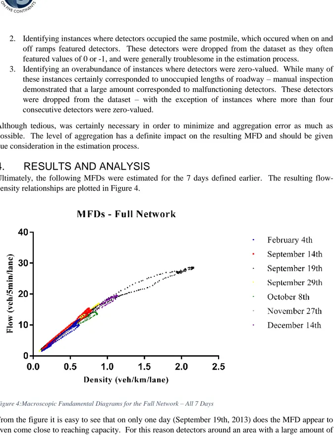
Ultimately, the following MFDs were estimated for the 7 days defined earlier. The resulting flow-density relationships are plotted in Figure 4.
Figure 4:Macroscopic Fundamental Diagrams for the Full Network – All 7 Days
From the figure it is easy to see that on only one day (September 19th, 2013) does the MFD appear to even come close to reaching capacity. For this reason detectors around an area with a large amount of demand (Seoul – a large metropolitan city) were isolated as seen in Figure 5.
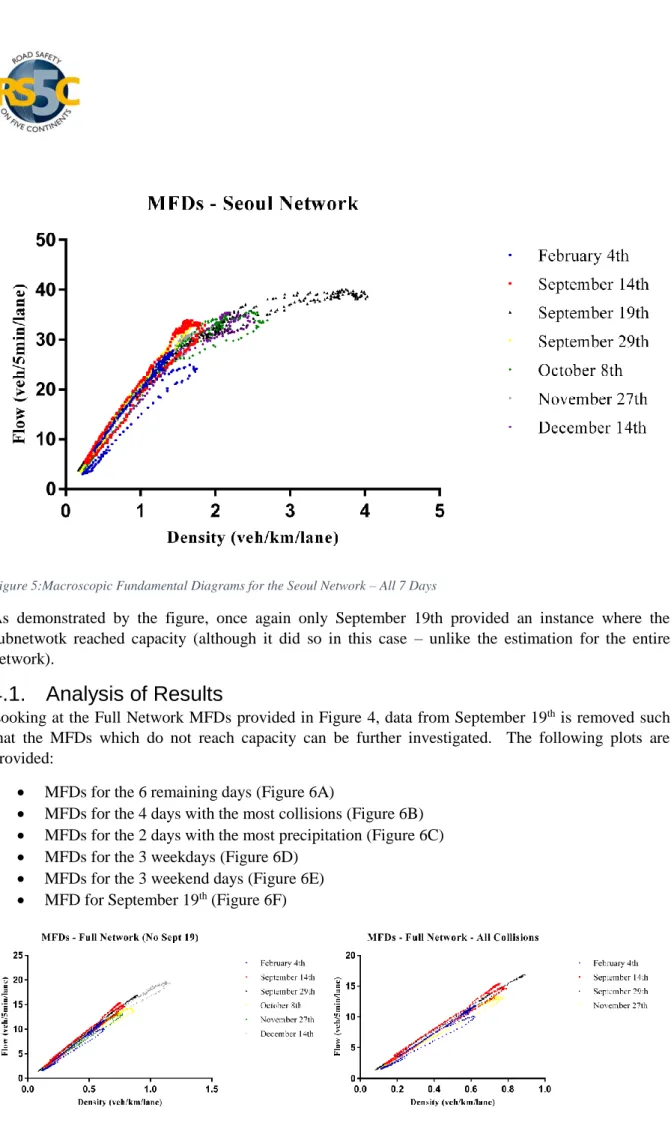
Figure 5:Macroscopic Fundamental Diagrams for the Seoul Network – All 7 Days
As demonstrated by the figure, once again only September 19th provided an instance where the subnetwotk reached capacity (although it did so in this case – unlike the estimation for the entire network).
4.1. Analysis of Results
Looking at the Full Network MFDs provided in Figure 4, data from September 19th is removed such
that the MFDs which do not reach capacity can be further investigated. The following plots are provided:
MFDs for the 6 remaining days (Figure 6A)
MFDs for the 4 days with the most collisions (Figure 6B) MFDs for the 2 days with the most precipitation (Figure 6C) MFDs for the 3 weekdays (Figure 6D)
MFDs for the 3 weekend days (Figure 6E) MFD for September 19th (Figure 6F)
Figure 6A-6F:Comparison of Macroscopic Fundamental Diagrams for the Full Network
Observation of Figure 6A demonstrates that for all days in which network capacity was not reached, the resulting MFD featured a “figure-eight” shaped hysteresis loops – which, as mentioned by Gayah and Daganzo (2011), are not as common a clockwise hysteresis loops, but not as rare as counter-clockwise loops. These loops occur when observed flows are higher during loading for high densities and lower during loading for low densities (Gayah & Daganzo, 2011); a phenomenon that makes logical sense when considering a highway network operating at flow conditions that do not reach network level capacity. For September 19th (the only day where the observed flow approached network
level capacity), the resulting hysteresis loop was clockwise (the most common and expected shape (Gayah & Daganzo, 2011)), and the resulting shape of the MFD was directly in line with expectation and previous research (Geroliminis & Sun, 2011). Additional investigation into the temporal nature of the estimated MFDs reveals that for the “figure-eight” hysteresis loops, the flow-density relationship follows the lesser slope between the hours of approximately 3 AM and 10 AM, continues to operate near the highest achieved flow/density values until approximately 6 PM at which the curve follows the higher slope back to its minimum achieved flow/density values. This temporal nature exhibited by the hysteresis loop is consistent with previous studies (Buisson & Ladier, 2009; Wang et al., 2015). Moving to Figure 6B, it is readily apparent that the two weekend days with the most collisions also featured the achievement of higher flow rates – most certainly due to the increased demand on these days (as compared to their weekday counterparts). The same can be observed in Figure 6C where the weather day that falls on a weekend (December 14th) exhibits a higher achieved flow rate. This result
is specific to the Full Network estimation, as expectation is that inter-city travel demand will increase on the weekends while intra-city demand should be more consistent regardless of the day of the week. Finally, inspection of Figures 6D and 6E indicates that in both cases the day featuring the most precipitation and the least number of collisions achieved the highest flow rates. Furthermore, comparison of these two figures demonstrates that the size and location of the hysteresis loop in the MFD changes based on the amount of demand. Increased demand “pushes” the hysteresis loop further up the flow – density curve and also reduces the size of the loop in the uncongested regime. This
result is further solidified through comparison with Figure 6F – where the network appears to be approaching capacity.
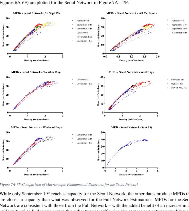
After having the MFD results presented for the Full Network in conformity with previous findings, the focus is then directed towards the Seoul Network only; data from September 19th is removed from the
Seoul Network and the six plot types outlined for the Full Network (above, see the definition of Figures 6A-6F) are plotted for the Seoul Network in Figure 7A – 7F.
Figure 7A-7F:Comparison of Macroscopic Fundamental Diagrams for the Seoul Network
While only September 19th reaches capacity for the Seoul Network, the other dates produce MFDs that
are closer to capacity than what was observed for the Full Network Estimation. MFDs for the Seoul Network are consistent with those from the Full Network – with the added benefit of an increase in the uniformity of daily demand across this subnetwork (reaffirming the comparison between weekday and weekend MFDs in the Full Network estimation). These results further support the analysis conducted above; indicating that days with increased collisions feature the largest disruptions in the MFD as well as the lowest achieved maximum daily flow rates across the network. Now, referring back to the estimated SEM, the initially counterintuitive result surrounding weather conditions is better understood. While weather may cause some disruption in the MFD – weather related events do not
restrict the maximum achieved flow rate on the network the way that an abundance of collisions or an increase in demand do. Furthermore, while infrastructure and traffic related characteristics also play a role in MFD disruption – these disruptions are again minimal when compared with those caused by collision, holiday or weather events.
5.
CONCLUSIONS AND FUTURE WORK
Research conducted in this study began with the estimation of a structural equation model based on collision data from 2011 to 2013 for the highway network in South Korea. The resulting model indicated that collisions and weather both had impacts on the time-dependent endogenous variables and based on these findings 7 specific days in 2013 were selected for additional investigation (days corresponding to the highest collision totals / precipitation totals plus one day corresponding to a large increase in network demand). Macroscopic Fundamental Diagrams were estimated for these 7 days by aggregating data from millions of loop detectors along the highway network in South Korea. Results demonstrated that on only one occasion (the day with the most demand, September 19th) did the Full
Network appear to nearly reach capacity. The shapes of all resulting estimations were then analyzed, and these plots demonstrated consistency with previous studies both in the general case of the shape and in the specific pattern of the hysteresis loops that formed within (clockwise for the day approaching capacity and figure-eight shaped elsewhere). In order to push the network towards capacity, additional estimation was conducted by isolating loop detector data around the city of Seoul. The MFDs estimated for the Seoul Network were consistent with those estimated for the Full Network and allowed for more detailed insights to be made (as the network operated at flow rates closer to capacity as compared to the Full Network estimations). Furthermore, results of the estimation conducted for the Seoul Network reaffirmed the findings of the structural model – as collisions had a greater impact on MFD disruption than did weather events.
MFD estimation is an area of research that is expanding rapidly; aided mainly by improvements in computing ability. Network level data such as that used for this study made up of millions of lines of data and is extremely difficult to work with – especially if there are inconsistencies in the dataset. Furthermore, given that MFD estimation is a relatively new practice – some questions still remain from a theoretical perspective. Future work should focus around creating a generalized estimation procedure as well as addressing some of the theoretical and analytical challenges such as the proper way to treat empty links within the network.
6.
ACKNOWLEDGEMENT
This material is based upon work partially supported by the National Science Foundation under Grant No. 1351647. Further support has been provided by the Simon Lee Endowment dedicated to encourage collaborative research between the George Washington University and Korea University. Any opinions, findings, and conclusions or recommendations expressed in this material are those of the author(s) and do not necessarily reflect the views of the National Science Foundation. The authors would also like to thank the Korea Highway Corporation for providing the data.
REFERENCES
AngloINFO Seoul (2015). Traffic congestion in Seoul City.
Bae, C (2013). Congestion pricing scheme in Seoul, Korea. http://blogs.ubc.ca/cindybae/2013/03/22/congestion-pricing-scheme-in-seoul-korea/. Accessed Jul. 21, 2015.
Buisson, C. and C. Ladier (2009). Exploring the Impact of Homogeneity of Traffic Measurements on the Existence of Macroscopic Fundamental Diagrams. Transportation Research Record: Journal of the Transportation Research Board, No. 2124, Transportation Research Board of the National Academies, Washington, D.C., 2009, pp. 127–136.
Cortina, J. (1993). What is Coefficient Alpha? An Examination of Theory and Application. Journal of Applied Psychology, 78(1), pp. 98-104.
Daganzo, C. (2007). Urban gridlock: Macroscopic modeling and mitigation approaches. Transportation Research Part B: Methodological, Vol. 41, No. 1, 2007, pp. 49–62.
Daganzo, C. F, and N. Geroliminis (2008). An analytical approximation for the macroscopic fundamental diagram of urban traffic. Transportation Research Part B, Vol. 42, 2008, pp. 771-781. Gayah, V. and C. Daganzo (2011). Clockwise hysteresis loops in the Macroscopic Fundamental Diagram: An effect of network instability. Transportation Research Part B: Methodological, Volume 45, Issue 4, May 2011, Pages 643–655.
Geroliminis, N., and C. F. Daganzo (2008). Existence of urban-scale macroscopic fundamental diagrams: Some experimental findings. Transportation Research Part B: Methodological, Vol. 42.9, 2008, pp. 759-770.
Geroliminis, N., and J. Sun (2011). Properties of a well-defined macroscopic fundamental diagram for urban traffic. Transportation Research Part B, Vol. 45, 2011, pp. 605–617.
Geroliminis, N., N. Zheng, and K. Ampountolas (2014). A three-dimensional macroscopic fundamental diagram for mixed bi-modal urban networks. Transportation Research Part C: Emerging Technologies, Vol. 42, 2014, pp. 168-181.
Golob, T. F. (2001). Structural Equation Modelling for Travel Behavior Research, Irvine: Institute of Transportation Studies, University of California Irvine.
Hamdar, S. H., H. S. Mahmassani and R.B. Chen (2008). Aggressiveness Propensity Index for Driving Behavoir at Signalized Intersections. Accident Analysis and Prevention, Volume 40, pp. 315 - 326. Hu, L. and P.M. Bentler (1998). Fit Indices in Covariance Structure Modeling: Sensitivity to Underparameterized Model Misspecification. Psychological Methods, pp. 424 - 453.
Ji, Y., W. Daamen, S. Hoogendoorn, S. Hoogendoorn-Lanser, and X. Qian (2010). Investigating the Shape of the Macroscopic Fundamental Diagram Using Simulation Data. In Transportation Research Record: Journal of the Transportation Research Board, No. 2161, Transportation Research Board of the National Academies, Washington, D.C., 2010, pp. 40-48.
Jia, E. C., W. Jianqiang, and D. Ni (2014). An Efficient Methodology for Calibrating Traffic Flow Models Based on Bisection Analysis. Journal of Applied Mathematics, 2014.
Knoop, V. L., S. P. Hoogendoorn, and J. W. C. Van Lint (2013). The impact of traffic dynamics on macroscopic fundamental diagram. Presented at the 92nd Annual Meeting Transportation Research Board, Washington, DC., 2013.
Korean Expressway Corporation (KEC) (2015). Expressway Construction. http://www.ex.co.kr/site/com/pageProcess.do; Accessed July, 2015
Leclercq, L., N. Chiabaut, and B. Trinquier (2014). Macroscopic Fundamental Diagrams: A cross-comparison of estimation methods. Transportation Research Part B, Vol. 62, 2014, pp. 1-12.
Mathew, T. V., and K. V. K., Rao (2006). Microscopic traffic flow modeling. Introduction to Transportation Engineering, 2006.
Mohan, R., and G. Ramadurai (2013). Heterogeneous Traffic Flow Modelling Using Macroscopic Continuum Model. Procedia-Social and Behavioral Sciences, Vol. 104, 2013, pp. 402-411.
Park, S. Road Accidents in Korea. IATSS research, Vol. 32.2, 2008, pp. 118-121.
RGB Spectrum (2008). New South Korean traffic management center keeps highway traffic flowing. http://www.rgb.com/fr/node/572. Accessed Jul. 21, 2015.
Ro, J. Infrastructure development in Korea. Infrastructure Development in Pacific Region, Osaka, Japan, 2002.
Sijtsma, K. (2009). On the Use, the Misuse, and the Very Limited Usefulness of Cronbach’s Alpha. Psychometrika, pp. 107 - 120.
Wang, P. F., K. Wada, T. Akamatsu, and Y. Hara (2015). An Empirical Analysis of Macroscopic Fundamental Diagrams for Sendai Road Networks. Interdisciplinary Information Sciences, Vol. 21.1, 2015, pp. 49-61.
World Health Organization (WHO) (2015). Road traffic deaths data by country. http://apps.who.int/gho/data/node.main.A997; Accessed July, 2015.
Yonhap News Agency (YNA) (2014). S. Korea road fatality rate second highest in OECD members. http://english.yonhapnews.co.kr/business/2014/07/07/99/0501000000AEN20140707002300320F.html ; Accessed July, 2015.
APPENDIX A: VARIABLE CODING FOR STRUCTURAL MODEL
Variable Description Details
General
Location Location of collision by
infrastructure
1: Main Line 0: Else 98: Blank
Severity Level Intensity of collision 1: A
2: B 3: C 4: D Collision Factor Technical cause of collision 1: Driver
2: Vehicle 3: Other 98: Blank Collision Type Variable corresponding to type of
collision involved 1: Vehicle-Vehicle 2: Vehicle-Person 3: Vehicle-Facility 98: Blank 99: Etc. Infrastructure
Road Pavement Type of pavement on roadway 0: Concrete 1: Asphalt Horizontal Alignment Type of horizontal curve 0: Straight
1: Curve Over 100 2: Curve 500-1000 3: Curve Under 500 Vertical Gradient Grade of incline/decline 0: Flat
1: Upgrade <1% 2: Upgrade 1-3% 3: Upgrade >3% 11: Downgrade <1% 12: Downgrade 1-3% 13: Downgrade >3% Pavement Condition Pavement material 0: Normal
1: Cracked, Plastic Deformation 2: Pot hole
98: Blank 99: Etc. Median Type Type of median on roadway 0: No Median
1: Green Area 2: Guardrail 3: Moving Wall 4: Protective Wall (81 cm) 5: Protective Wall (127 cm) 98: Blank 99: Etc. Shoulder Type Type of shoulder barrier on
roadway
0: None
1: Fence for Falling Stones 2: Guardrail, Guard Cable, Guard Pipe, Guard Fence
3: Concrete Wall 98: Blank 99: Etc.
Environmental
Precipitation Type of weather conditions present during collision
0: No Precipitation and No Fog 1: Precipitation or Fog
98: Blank Day and Night Variable corresponding to time of
day during collision
0: Day 1: Night 98: Blank Surface Condition Moisture conditions on surface
from weather
0: Dry 1: Wet, Snow 99: Etc. Lighting Variable corresponding to lighting
conditions
0: Daytime, on
1: Malfunction, no light 98: Blank
Driver and Vehicle
Vehicle Type at Fault/Victim Type of vehicle involved 1: Sedan 2: Van 3: Trailer 4: Freight 98: Blank 99: Special, Etc. Gender of Driver Variable corresponding to driver’s
gender
0: Male 1: Female Age of Driver Variable corresponding to driver’s
age 1: Under 20 2: 20 – 30 3: 30 – 40 4: 40 – 50 5: 50 – 60 6: 60+ 98: Blank 99: Other, Etc. Driver’s Condition Level of alertness or physical
condition of driver
0: Normal
1: Drug Use, Alcohol
2: Watching DMB, Cell Phone, Equipment Manipulation 3: Fatigue
4: Disease, Mental Disorder 5: No License
98: Blanks 99: Etc.