COMADEM 2014
2 7t h I n t e r n a t i o n a l C o n g r e s s o f C o n d i t i o n M o n i t o r i n g a n d D i a g n o s t i c E n g i n e e r i n g
Optimum inspection interval for hidden functions during extended life
Alireza Ahmadi
a1, Behzad Ghodrati
bAmir.H S.Garmabaki
cand Uday Kumar
dabcd Luleå University of Technology, Luleå, Sweden
———
1 Corresponding author. Tel.: +46-920-493047; e-mail: alireza.ahmadi@ltu.se
P A P E R T E X T
The methodology proposed in this paper aims to provide a mathematical model for defining optimal Failure Finding Inspection (FFI) interval, during the extended period of the replacement life. It considers the maintenance strategy of “a combination of FFI, and a discard action after a series of FFI”. A cost function (CF) is developed to identify the cost per unit of time associated with different FFI intervals, for the proposed extended period of life, i.e. postponement period. The Mean Fractional Dead Time (MFDT) concept is used to estimate the unavailability of the hidden function within the FFI intervals. The proposed method concerns as-bad-as-old (ABAO) inspection and repairs (due to failures found by inspection). This means that the unit keeps the state which it was in just before the failure, that occurred prior to inspection and repair. It also considers inspection and repair times, and takes into account the costs associated with inspection and repair, the opportunity cost of lost production due to maintenance downtime created by inspection and repair actions, and also the cost of accidents due to the occurrence of multiple failure.
Notation and Acronyms α scale parameter β shape parameter
φ demand rate for the hidden function per hour CA cost of an accident
CI cost of inspection
COC opportunity cost of lost production
Cr cost of repair
CRep cost of Discard
FFI Failure Finding Inspection F(t) unreliability function
FN(t) conditional probability of failure within the Nth FFI cycle
h(t) rate of occurrence of failure (ROCOF) H(t) cumulative ROCOF
K Number of scheduled FFI interval MFDT Mean Fractional Dead Time N number of extended FFI cycles R(t) reliability function
t local time within Nth inspection cycle
T inspection interval TI inspection time
TK scheduled discard life with TK=TS.K
TN extended discard life (postponement period) with TN=TP.N
TP FFI interval for the extended life period
TR repair timeTS original scheduled FFI
interval
1. Introduction
One aspect of maintenance programme analysis by Reliability-Centerd Maintennace (RCM) methodology, is to develop tasks to preserve and assure the availability of hidden functions (or off-line functions). These types of functions are used intermittently or infrequently, so their failure will not be evident to the operating crew during the performance of normal duties1. Examples are the failure of a pressure relief
valve, fire detector, fire extinguisher or emergency shutdown system. Termination of the ability to perform a hidden function is called hidden failure.
Hidden failures are analyzed as part of a multiple failure. A multiple failure is defined as “a combination of a hidden failure and a second failure or a demand that makes the hidden failure evident”. Hence, hidden failures are not known unless a demand is made on the hidden function as a result of an additional failure or second failure, i.e. a trigger event, or until a specific operational check, test or inspection is performed1-2.
Depending on the criticality and consequences of multiple failures and the demand rate, a specific level of availability of the hidden function is needed. Obviously, the probability of a multiple failure can be reduced by reducing the unavailability of the hidden function by performing a maintenance/ inspection task.
Hidden failures are divided up into the “safety effect” and the “non-safety effect” categories. The failure of a hidden function in the “safety effect” category involves the possible loss of the equipment and/or its occupants, i.e. a possible accident. The failure of a hidden function in the “non-safety effect” category may entail possible economic consequences due to the undesired events caused by a multiple failure (e.g. operational interruption or delays, a higher maintenance cost, and secondary damage to the equipment).
According to (RCM)1,3,4 a scheduled Failure Finding
Inspection (FFI) may be necessary to detect the functional failure of hidden functions that has already occurred, but is not evident to the operating crew. The FFI tasks are developed
to determine whether an item is fulfilling its intended purpose. In fact, if a hidden failure occurs while the system is in a non-operating state; the system’s availability can be influenced by the frequency at which the system is inspected5. If inspection
finds the system inoperable, a maintenance action is required to repair it.
When the unit is aging, it may not be possible to find a single FFI task which, on its own, is effective in reducing the risk of failure to a tolerable level for the whole life cycle. This is due to the fact that, in a long run, the unavailability of hidden functions within inspection interval may exceed the acceptable limit (see Section 3). Therefore, as a common practice, when a single FFI task is not effective, it is necessary to employ a replacement task after a series of FFI to reduce the risk of multiple failures. See 6,7 for further study .
In fact, due to operational restrictions, or a lack of resources, sometimes the operators cannot ground the equipment, to perform the replacement task, as scheduled. In these cases, the operators are willing to postpone the replacement task to the earliest possible opportunity so that their operation will not be affected. However, such a postponement would affect the risk and may incur unacceptable economical, operational or safety risks. Hence, a trade-off analysis is needed to evaluate whether the extension of the discard life is acceptable. If the life extension justified, the inspection interval, also should be adjusted for the period of life extension. Moreover, safety and risk management should also be based on cost-benefit analyses performed to support decision making on safety investments and the implementation of risk reducing measures. Cost-benefit analysis is seen as a tool for obtaining efficient allocation of resources, by identifying which potential actions are worth undertaking and how these actions should be carried out. Aven and Abrahamsen 8 argue that by adopting the
cost-benefit method the total welfare will be optimized.
The methodology proposed in this paper aims to provide a mathematical model for defining optimal FFI interval, during the extended period of the replacement life. It considers the maintenance strategy of “a combination of Failure Finding Inspection (FFI), and a discard action after a series of FFI”. A cost function (CF) is developed to identify the cost per unit of time associated with different FFI intervals, for the proposed extended period of life, i.e. postponement period. The Mean Fractional Dead Time (MFDT) concept is used to estimate the unavailability of the hidden function within the FFI intervals, see 9. The proposed method concerns as-bad-as-old (ABAO)
inspection and repairs (due to failures found by inspection). On the other hand, the unit keeps the state which it was in just before the failure that occurred prior to inspection and repair. It considers inspection and repair times, and takes into account the costs associated with inspection and repair, the opportunity cost of lost production due to maintenance downtime created by inspection and repair actions, and also the cost of accidents due to the occurrence of multiple failure.The rest of the paper is constructed as follow. In section 2, probabilistic models for repairable units is discussed and in section 3, proposed analytucal model is presented. The paper ends in chapter 4 with the conclusion. This paper is an extended version of Ahmadi, et al. 10.
COMADEM 2014 β β N(t) 1 exp (α 1)T ( α1)T t F TK N P TK N P
2. Probabilistic Models for Repairable Units
In actual fact, the failure of a unit may be partial, and a repair resulting from findings during FFI may be a partial repair and mostly concern adjusting, lubricating or cleaning the item. These types of repairs provide only a small additional capability for further operation, and do not renew the unit or system and may result in a trend of increasing failure rates11.
In this study, it is considered that repair resulting from findings during FFI will be partial repair, i.e. minimal repair, and hence the unit returns to an “as-bad-as-old” state after inspection and repair actions. On the other hand, the unit keeps the state which it was in just before the failure that occurred prior to inspection and repair, and the arrival of the ith failure is conditional on the cumulative operating time up
to the (i-1)th failure. Hence, in the present study the power law
process have been selected to model the reliability of such repairable units.
Under the imperfect repair assumption, the rate of occurrence of failure (ROCOF) and associated cumulative ROCOF of the power law are defined as 1213:
1 ( ) t h t (1) ( ) t H t (2)
where α and β denote the scale and shape parameters, respectively. Consequently, the failure probability (unreliability) and reliability functions at time “t” are defined as: ( ) ( ) H t exp t R t e (3) ( ) ( ) 1 ( ) 1 H t 1 exp t F t R t e (4)
In fact, if during the scheduled FFI, the unit is found functional (i.e. is found survived) at the (k-1)thinspection, the
conditional probability of failure at any time “t”, within the kth
inspection cycle is given by:
k ( 1) ( 1) F ( ) 1 expt K TS K TS t (5)
where “t” denotes the local time within the Nth inspection
cycle, and TS denotes the original scheduled FFI interval.
3. PROPOSED ANALYTICAL MODEL:
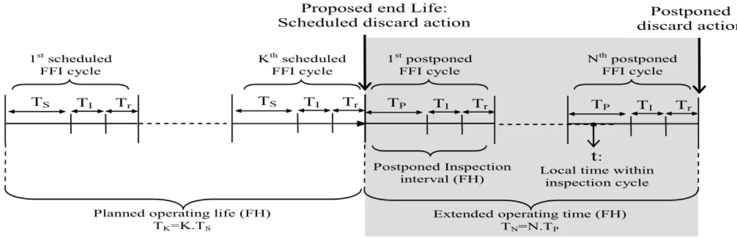
Figure. 1 shows a schematic description of maintenance events during the planned and extended operating times. During the initial planned operating life, the system must be grounded to perform an inspection task each time an accumulated number of operating hrs “TS” has been reached.
The first inspection is performed after “T” hours, and consequently the Kth inspection will be performed after “T
K”
operating hours. The inspection task takes TI hours and, in
the case of a finding which leads to a repair, the repair takes
Tr hours. Hence, an inspection cycle includes T, TI and Tr. An
expected operating hours, “TK”, is considered as the unit’s
planned operating life, and is divided into K inspection cycles with the inspection interval TS, so that TK=K.TS .
Based on the selected interval, when the item reaches the maximum allowable operating hours, after which it will exceed the allowable risk limit, the item should be restored to its original condition. In this situation, when the operator wants to have an extension time, TN, added to the planned
operating life (i.e. age, TK) the conditional probability of
failure at time “t” after TK and within the Nth inspection cycle
of the extended operating time, is given by:
(6) where, under the postponement strategy, “t” denotes the local time within the Nth inspection cycle, and T
P denotes the FFI
interval; both under postponement strategy.
The unavailability of hidden functions is usually measured by the mean fraction of time during which the unit is not operational as protection, i.e. the Mean Fractional Dead Time (MFDT)2 . If dormant failures occur while the system is
in a non-operating state, the system availability can be influenced by the frequency at which the system is inspected.
TS TI Tr TS TI Tr 1st scheduled FFI cycle K th scheduled FFI cycle TP TI Tr
Extended operating time (FH) TN=N.TP Nth postponed FFI cycle Postponed discard action TP TI Tr Postponed Inspection interval (FH) 1st postponed FFI cycle
Proposed end Life: Scheduled discard action
t:
Local time within inspection cycle Planned operating life (FH)
TK=K.TS
4
Note that inspection, cannot improve the reliability, but can only improve the function availability5. According to Rausand
and Vatn 9 and Vaurio 14, the function unavailability at time
“t” within the Nth inspection cycle is equal to the conditional
probability function, i.e. FN(t). Consequently, the mean
interval unavailability within the Nth inspection cycle of the
extended operating time, with FFI at every “T” hours, is given by: (T,N) 0 1 MFDT ( ) T N F T dt T
(7)3.1. Cost function for postponed FFI
The analytical model presented in this paper is based on the following assumptions:
1) The inspection and repair times associated with findings through FFI, i.e. Ti and Tr (constant values), do
not change with operating time.
2) The failures concerned are not evident to the operating crew and hence do not interrupt the operation when they occur.
3) The failures are completely detectable by inspection/testing.
4) The inspection does not create failure by the nature of the tasks involved.
5) The maintenance crew do not create failure by their own actions.
6) Postponement of a restoration task does not increase the degradation and restoration costs.
The following cost parameters are considered for cost modelling of FFI in the postponement scenario:
Direct cost of inspection task, Ci. This is considered as a
deterministic value and as a constant in consecutive inspection cycles.
Cost of possible repair due to a finding, Cr. As the system
is undergoing aging, the probability of failure will change in consecutive inspection cycles. Hence, the expected repair cost within the Nth postponed inspection cycle can
be estimated as: Cr . FN (TP).
Cost of an accident, due to multiple failures, CA. The
expected value of CA in the Nth inspection cycle depends
on the expected time during which the function is not available between two postponed inspections, “MFDT(T,N).T”, and the demand rate for the unit, φ, i.e.
“CA . φ .MFDT(TP,N) .T”. For the “safety effect” category,
CA refers to the cost of accidents, e.g. the possible loss of
the equipment and/or its occupants. For the “non-safety effect” category, CA may entail possible economic
consequences due to the undesired events caused by a multiple failure (e.g. operational interruption or delays, a higher maintenance cost, and secondary damage to the equipment.
Opportunity cost of the system’s lost production, Coc.
This cost is associated with the total system downtime due to inspection and repair, i.e. Ti and Tr. The expected
value can be estimated as: COC .[TI+Tr.FN(T)]
Summing up, the total cost for a series of “N” inspection cycles under the FFI postponement strategy can be estimated by:
P , Rep 1 (T , ) . ( ) . . ( ) . .MFDT . P N I r i P oc I r i P T N i A i P C C F T C T T F T C C C T
(8)and the cost rate function for the extended period of time can be estimated by:
( , )T NP ( , )T NP N
CRF C T (9)
MAPLE Software is used to enable variation of the parameters of (9) to identify the cost per unit of time considering a target operating time of TK=6000Hrs and
TN=1000, with the selected values of α=1000, β=3, CA.φ=1,
CI=10, Cr=15, COC=100, Ti=0.2, and Tr=0.3, CRep=2000.
As Fig. 9 shows, the CRF is not sensitive around absolute Top (i.e. 21,7Hrs), meaning that a range of inspection intervals,
i.e. Top ε [19Hrs-25Hrs], is reasonably acceptable.
Figure 2:
In fact, the CRF is just the additional cost per unit of time for the extended operating life. If the number of inspections during extended life period tends to infinity (N →∞), then the CRF can be expected as:
. . , 1 1 . . 1 . . lim . ( ) lim . . . lim . ( ) lim P oc i i r P P P C T Cr oc i T TP P oc r P Coc rT TP T N N N N oc I r N P i i i P P i N N C NT C C N NT NT T N oc r A N P i P N C T N NT Lim CRF C NC C Lim F T T NT NT NT C T C F T NT Re ( , ) 1 . 0 , N . (10) .( ) . P A P N s P T N i P P N N C i r oc i r A T P N C T MFDT NT NT C C C T T Lim CRF C T
COMADEM 2014
3.2. Optimum interval
In fact, the operating time TN is divided into N inspections
with the interval TP, so that TN=N.TP. The following equations
are valid under certain conditions for FN(T), as proved by
Vaurio 14: 0 ( ) ( ) K i K i F T H T
(11) 2 ) ( ) ( 0 ) , ( 0 K K i K T K i i T H MFDT T F
(12)Fi(T) represents the conditional probability of having just
one failure in the ith inspection interval, provided that the unit
found functional at (i-1)th inspection. H(T
K) represents the
mean number of failures over an interval of (0,TK). Hence, it
is evident that H(TN) overestimates ΣFi(T). It shold ne noted
that for larger α, and smaller β values, the H(TK) and FN(T)
become more close, and tend to lead to more accuracy in the estimation, while smaller α and larger β values tend to lead to more deviation in the estimation. Moreover, selecting larger T values increases the inaccuracy in the estimation.
Similarly, we can express the mean number of failures within the extended operation time TP as follow:
0 ( ) ( ) ( ) N i K P P j F T H T T H T
(13) (13) ( , ) 0 0 ( ) ( ) ( ) 2 N N K P P i T K i i H T T H T F T MFDT
(14) Likewise, using the method introduced by Vaurio 14, by
substituting (13) and (14) into (9), and denoting TP.N as TN,
the following CRF can be derived as a function of the inspection interval T, and the operating time TP:
The optimum inspection interval, TOP, that can minimize
the CRF, by a fixed operating time, TN (Hrs), can be found
through this derivative [CRF(T,N)/dTP]=0:
(16)
In accordance with (16), and considering a target operating time of TK=6000Hrs, extended operating time of TN=1000,
and with the selected values used in Fig. 2, the optimum inspection interval is estimated to Top=25.xx Hrs, which leads to CRF=$0.209 with N=40 [1000/25=40].
However, in case of the “safety effect” category of failure, the postponement process requires adequate proof of risk reduction which satisfies the risk limits. Since such a postponement may increase the cost rate and affect economy negatively, another tradef-off analysis is needed to evaluate
whether the postponement idea is economical and is acceptable or not.
In the case of the “safety effect” category of failure, the limit conditions for the risk of multiple failures may be dictated through the policies authorities or the companies themselves. Considering Rmax as the maximum permissible
risk limit for the probability of multiple failures, then the postponement process needs to limit the risk of failure under the following supplementary constraint:
(T, ) max ( , ) max
.MFDT N R MFDT T N R /
(17)
4. Conclusions
This paper introduces a methodology to identify the optimum Failure finding inspection (FFI) interval during extended operating life of a nunit. In this study, a cost function (CF) has been developed to identify the cost per unit of time associated with different FFI intervals, for the proposed extended period of life. Moreover, a mathematical model has been defined to obtain the optimal FFI interval, during the extended period of the replacement life. Following this methodology, the optimum FFI interval that generates the lowest cost per unit of time, can be obtained.
The interval unavailability behavior has been discussed and MFDT has been used to identify the limits by which the risk of failure can be eliminated. This approach makes it possible to recognize the real effect of postponement on the total maintenance cost and to evaluate whether performing postponement provides benefits. Following proposed methodology enhance one’s capability to take correct and effective decisions on the postponement of discard tasks. Bibliography
Dr. Alireza Ahmadi is an Associate Professor at the Division of Operation, Maintenance Engineering, Lulea University of Technology, Sweden, where he got his PhD and did his postdoctoral research in the area of reliability and maintenance engineering. He developed, led and participated in several research projects, within the areas of reliability, maintainability, maintenance program development and dependability. He is supervising a number of doctoral students and has published a number of papers in peer-reviewed journals and conferences. His research interests include reliability engineering and system safety assessment; maintenance program development and optimization; and Reliability Centered Maintenance. Alireza has more than 12 years of experience in civil aviation maintenance as senior licensed engineer and served as manager with Production Planning and Control department in airlines.
Dr. Behzad Ghodrati, is Associate Professor at Lulea University of Technology, Division of Operation and Maintenance Engineering. He holds a Ph.D. in Reliability and Product support from the same university, Sweden. Dr. Ghodrati's work is directed to reliability based product support. His main focus is on the forecasting and estimation of required spare parts for industrial systems.
Dr. Garmabaki is Assistant Professor at the Department of Computer Science, Islamic Azad University, Nour Branch. He currently joined to Lulea University Technology, Sweden as post-doctoral researcher. He obtained his PhD and M.Sc.
2 1 . . ) . ( . 2 ) H(T ) T H(T C T C C T T K N K A I oc I N OP
Re (15) 2 r K N K I T,N P N oc r K N K oc I P N p A P K N K N N C H(T T ) H(T ) C CRF T T C .T . H(T T ) H(T ) C .T T T C C . .T . H(T T ) H(T ) T T 6
degrees from the University of Delhi, India in 2013 and University of Kerman, Iran in 2001. He has published several papers in international journals and conferences proceedings. His research interests include Reliability Engineering, Software Reliability, Marketing, and Fuzzy Optimization.
Dr. Uday Kumar is Professor of Operation and Maintenance Engineering at Luleå University of Technology, Luleå, Sweden. His research and consulting efforts are mainly focused on enhancing the effectiveness and efficiency of maintenance processes at both the operational and the strategic levels, and visualizing the contribution of maintenance in an industrial organization. He has published more than 175 papers in peer-reviewed international journals and conference proceedings, as well as chapters in books. He is a reviewer and member of the Editorial Advisory Boards of several international journals. His research interests are maintenance management and engineering, reliability and maintainability analysis, and life cycle cost.
Acknowledgments
We would like to acknowledge gratefully the financial support provided by the Luleå Railway Research Center to perform this study.
References and notes
1. Moubray, J., Reliability Centered Maintenance. Oxford:
Butterworth-Heinemann, 1997.
2. Rausand, M.; Høyland, A., System Reliability Theory:
Models, Statistical Methods, and Applications. Wiley: Hoboken, NJ
2004.
3. IEC, 60300 (3-11): Application Guide - Reliability Centred Maintenance. International Electrotechnical Commission: Geneva, 1999.
4. SAE-JA1012, A Guide to the Reliability-Centered Maintenance (RCM) Standard,. Society of Automotive Engineers: Warrendale, 2002.
5. Ebeling, C. E., An Introduction to Reliability and
Maintainability Engineering. 2 ed.; Waveland Press: 2010.
6. Ahmadi, A.; Kumar, U., Cost Based Risk Analysis to Identify Inspection and Restoration Intervals of Hidden Failures Subject to Aging. Reliability, IEEE Transactions on 2011, 60 (1), 197-209.
7. Ahmadi, A. Aircraft Scheduled Maintenance Program Development: Decision Support Methodologies and Tools. Luleå University of Technology, 2010.
8. Aven, T.; Abrahamsen, E., On the use of cost-benefit analysis in ALARP processes,. International Journal of
Performability Engineering 2007, 3 (3), 345-353.
9. Rausand, M.; Vatn, J., Reliability modeling of surface controlled subsurface safety valves. Reliability Engineering &
System Safety 1998, 61 (1–2), 159-166.
10. Ahmadi, A.; Ghodrati, B.; Rantatalo, M. In Optimum
Failure Finding Inspection During Extended Operation Life, In
proceeding of the 3rd International Conference on Recent Advances in Railway Engineering (ICRARE), Tehran, Iran, , Apr 30- May 1; Tehran, Iran, , 2013.
11. Modarres, M., Risk Analysis in Engineering: Techniques, Tools, and Trends. Taylor & Francis: Boca Raton, USA, 2006.
12. Ascher, H.; Feingold, H., Repairable Systems Modelling,
Inferences, Misconceptions and their causes. Marcel Decker: New
York, 1984.
13. Klefsjo, B.; Kumar, U., Goodness-of-fit tests for the power-law process based on the TTT-plot. Reliability, IEEE
Transactions on 1992, 41 (4), 593-598.
14. Vaurio, J. K., On time-dependent availability and maintenance optimization of standby units under various
maintenance policies. Reliability Engineering & System Safety 1997,