www.transportekonomi.org
The impact of cumulative tonnes on track failures: An
empirical approach
Kristofer Odolinski, VTI
Working Papers in Transport Economics 2019:1
Abstract
Cost-benefit analysis is often used in appraisal of rail infrastructure investments. A corresponding decision support is, however, not available for rail infrastructure maintenance and renewal. To for example decide whether to renew or continue to maintain an infrastructure asset, a relationship between cumulative traffic and infrastructure failures is required. This relationship is established in this paper, using an empirical (top-down) approach on Swedish data for years 2003 to 2016. It is shown that the average elasticity for track failures with respect to cumulative tonnes is 0.32, and that the elasticity varies for different levels of traffic and for different infrastructure characteristics. The results in this paper can for example be used to calculate the impact cumulative tonnes have on train delay costs, which together with a relationship between cumulative traffic and infrastructure maintenance costs are essential in an economic optimization of maintenance and renewal activities.
Keywords
Rail infrastructure; Track failures; Cumulative traffic; Infrastructure management
JEL Codes
1
The impact of cumulative tonnes on track failures: An empirical
approach
Kristofer Odolinski, the Swedish National Road and Transport Research Institute, VTI; Box 55685; 102 15 Stockholm, Sweden (kristofer.odolinski@vti.se)
Abstract
Cost-benefit analysis is often used in appraisal of rail infrastructure investments. A corresponding decision support is, however, not available for rail infrastructure maintenance and renewal. To for example decide whether to renew or continue to maintain an infrastructure asset, a relationship between cumulative traffic and infrastructure failures is required. This relationship is established in this paper, using an empirical (top-down) approach on Swedish data for years 2003 to 2016. It is shown that the average elasticity for track failures with respect to cumulative tonnes is 0.32, and that the elasticity varies for different levels of traffic and for different infrastructure characteristics. The results in this paper can for example be used to calculate the impact cumulative tonnes have on train delay costs, which together with a relationship between cumulative traffic and infrastructure maintenance costs are essential in an economic optimization of maintenance and renewal activities.
JEL codes: H54, L92, R49.
2 1. Introduction
Ensuring economically efficient transport services requires a rail infrastructure manager (IM) to efficiently allocate its resources with respect to the expected benefit of (rail) transport and the expected costs. The costs comprise investment, maintenance and renewal costs, as well as the railway users’ transport time costs. A determining factor for these costs is the condition of the railway assets, controlled by the IM. That is, a certain asset condition implies a certain level of costs for a given traffic volume. Hence, to minimize the costs over an asset’s life cycle, the IM needs information on the impact that asset condition has on transport time costs as well as maintenance and renewal costs.
What are proper measures on asset condition in this respect? This may differ for the different parts of the railway infrastructure, such as the track superstructure, substructure, signalling system, telecommunication and energy supply. In general, proper measures should be applicable as input in the prediction of an event (defects, failures, train delays etc.) and its associated costs. For track superstructure, measurements of the damage mechanisms wear, rolling contact fatigue, component fatigue and track settlement can provide a view on the asset’s current status (see for example Öberg et al. (2007)). It is (mainly) traffic accumulating over time that has caused these damages, which can vary depending on the characteristics of the railway and thus require different activities to minimize costs. Still, the damage mechanisms are to a large extent correlated (with traffic) and establishing their relative contribution to events and costs may therefore be difficult (see for example Smith et al. (2016)). Moreover, the maintenance activities that are carried out to rectify the damages do not restore the infrastructure asset to its original condition; maintenance is prolonging the lifetime of the asset, but the asset is still coming closer to the end of its life cycle as traffic is accumulating, with increasing maintenance and transport time costs (delay costs). Cumulative traffic may therefore serve as a useful indicator for track superstructure condition.
The events considered in this paper are track failures. In particular, the purpose of this study is to estimate the impact of cumulative tonnes on track failures. The aim is that the results can be used as input in a maintenance and renewal strategy, improving the allocative efficiency of infrastructure provision.
The Swedish infrastructure manager (Trafikverket) has requested results on the impact of cumulative tons on track failures for tracks with different track quality classifications – that is, tracks with different line speeds and different requirements on track geometry standards. Such results may be useful in a maintenance and renewal strategy if they can show the impact traffic has on the expected number of track failures when changing the quality classification on a track with a certain cumulative tonnage. Estimations in this paper are therefore carried out for different quality classifications. Moreover,
3 interactions with other technical aspects of the infrastructure are considered in the estimations, namely sleeper type and weight of the rails.
There is a wide literature on the prediction of railway failures, using either a mechanistic (bottom-up) approach or an empirical (top-down) approach. Examples of the former are Orringer et al. (1988), Jeong (2003), Hokstad et al. (2005), Podofillini et al. (2006), while examples of the latter are Dick et al. (2003), Schafer and Barkan (2008), Arasteh Khouy et al. (2014), Parra et al. (2012) and Zarembski et al. (2016). Many of these studies consider one type of track failures, such as deviations in track geometry (Arasteh Khouy et al. (2014), Zarembski et al. (2016)), broken rails (Dick et al. 2003, Hokstad et al. (2005), Schafer and Barkan (2008)), weld failures (Zhao et al. (2006)), and use predictions of failures to calculate optimal intervals for inspections and/or maintenance activities carried out to fix the specific defect or failure. Indeed, there are various failures and defects that can occur due to the different damage mechanisms (see for example Trafikverket (2014) or UIC (2002) for an overview of rail defects). In this paper, we include all damages that has resulted in a track superstructure failure. That is, in addition to rail failures and track geometry deviations, we also include failures related to sleepers, the fastening system, joints and ballast (however, failures on switches and crossings are not included). Hence, this paper analyses track failures at a high level of aggregation, with results that can be used in an overall maintenance and renewal strategy rather than being used for optimizing the timing of specific maintenance activities such as grinding or tamping. Our approach is more in line with the study by Gaudry et al. (2016), who consider the overall track degradation, where the marginal productivity of maintenance activities is reduced as the number of activities increases, which eventually makes a renewal necessary.
Specifically, the results in this paper are intended to be used in an economic optimization model for track maintenance and renewals. A strategy for developing such a model for the Swedish road and rail infrastructure was set out by Andersson et al. (2011), while Andrade and Teixeira (2011), Gaudry et al. (2016) and Sousa et al. (2018) are examples of models developed for railway infrastructure. In particular, the impact cumulative tonnes have on train delaying failures can be used to predict the train users’ delay costs (which however requires a model for how a train delaying failure affects train delays; see for example Jiang and Persson (2016)). Together with the effect cumulative tonnes have on track maintenance costs, the results can be used to assess the optimal timing of a track renewal. The impact cumulative traffic has on non-train delaying failures with respect to different infrastructure characteristics, such as line speeds and rail weights, may also be useful when planning the level of maintenance resources for different parts of the railway network.
4 A contribution of our paper is that we use cumulative tonnes in the estimation of track failures. We have access to a long panel dataset with track failures and infrastructure characteristics for the Swedish state-owned railway network (years 2003 to 2016), as well as traffic data from years 1900 to 2016 (yet, at different levels of aggregation, see section 2 below). Here we can note that Gaudry et al. (2016) also used cumulative tonnes in their study, based on current traffic levels in the first period of their dataset (1999) and multiplied by time (age of rails), while annual traffic for years up to 2007 are used to calculate cumulative traffic for years after 1999. The method and dataset used in our paper to calculate cumulative tonnes is more detailed (see section 2). Furthermore, a contribution of this paper is that we separate train-delaying failures and non-train delaying failures and estimate the impact cumulative traffic has on each of these types of failures.
The paper is organised as follows. In section 2, the calculation of cumulative tons is described, while the data is presented in section 3. The method and the model specifications are provided in section 4. Results are presented in section 5, while section 6 concludes.
2. Calculation of cumulative tonnes1
The Swedish railway network includes rail that were laid as early as around year 1900. To calculate cumulative traffic, it is necessary to have information about traffic since that year. However, the level of detail of the available traffic data varies, with data for years 1900-1998 at the national level and 1999-2016 at the track section level. Hence, for sections of rail that were laid earlier than 1999, we need to extrapolate the tonnage based on data at the national level. The basis for this extrapolation is the relative size of the national traffic volumes for years 1900-1998 with respect to the national traffic volume in year 1999. We account for variations in the size of the Swedish railway network by using total track length to calculate tonne densities (tonne-km/track-km) for the entire network. Specifically, for year 𝑡 = 1900, … , 1998, the tonne density for each section is calculated as
𝑄𝑖𝑡𝑑𝑒𝑛=
∑ 𝑄𝑁𝑖 𝑖𝑡𝑑𝑒𝑛 ∑ 𝑄𝑁 𝑖1999𝑑𝑒𝑛
𝑖 𝑄𝑖1999
𝑑𝑒𝑛 , (1)
where 𝑖 = 1, … , 𝑁 track sections and 𝑄𝑑𝑒𝑛 is tonne density. Thus, ∑ 𝑄𝑁𝑖 𝑖𝑡𝑑𝑒𝑛 represents tonne density
for the entire railway network. Information on rail age is available at a more disaggregate level than
5 track sections; each section comprise on average about 14 segments with rails inserted at various dates.
The traffic volumes available at the national level are freight gross tonne-km and passenger-km, where the former is used in extrapolating freight gross tonnes and the latter in extrapolating the passenger gross tonnes. Clearly, passenger-km is not ideal to use in this approximation. However, a correlation coefficient at 0.96 between passenger-km and passenger tonne-km (based on data for years 2005 to 2017) 2 indicates that passenger-km is adequate for an approximation of cumulative use in this respect.
Clearly, the use of traffic at the national level prior to year 1999 adds uncertainty to the calculation of cumulative tonnes, where older rails imply more uncertainty. However, in year 1999 and onwards, a majority of the tracks had been inserted after 1979. Table 1 presents the average year when the rail was inserted together with shares of tack lengths for different intervals for when the rail was inserted. Furthermore, there are rails that have been reused, which is not indicated in (most of) the available rail data. However, in year 2016, the rail data indicates the construction year along with the year the rail was inserted. When the difference between the construction year and the installation year is significant, one can infer that the rail is reused. If we consider a 10-year difference or longer to be an indication of a reused rail, then about 3 per cent of the tracks in year 2016 in our sample have been reused. The weighted average of the difference between construction year and installation year for rails with at least a 10-year difference is almost 28 years. There is no information available for where this rail was inserted before it was reused. We are therefore not able to calculate the cumulative tonnage prior to the them being inserted on the new location. Hence, for these rails, the actual cumulative tonnage is underestimated.
2 Official statistics on the gross tonne-km of passenger wagons from 2005 and onwards are made available by
6
Table 1. Year when rail was inserted, observed rail data in years 1999 to 2016. Year when rail
data is observed
Year when rail was inserted, weighted average
Per cent of rail inserted in year
1900-1919 1920-1939 1940-1959 1960-1979 1980-1998 1999- 1999 1982 0.3% 0.4% 3.5% 32.9% 62.6% 0.2% 2000 1983 0.0% 0.4% 3.0% 30.1% 64.5% 2.0% 2001 1984 0.0% 0.3% 2.9% 27.6% 65.7% 3.6% 2002 1985 0.0% 0.3% 2.6% 26.5% 65.4% 5.3% 2003 1985 0.0% 0.3% 2.3% 25.7% 64.7% 7.0% 2004 1986 0.0% 0.1% 2.2% 24.4% 64.0% 9.4% 2005 1987 0.0% 0.0% 2.1% 23.3% 63.0% 11.5% 2006 1987 0.0% 0.0% 2.0% 22.4% 62.3% 13.2% 2007 1988 0.0% 0.0% 1.9% 21.6% 61.3% 15.2% 2008 1988 0.0% 0.0% 1.9% 21.1% 60.6% 16.4% 2009 1988 0.0% 0.0% 1.6% 20.6% 59.5% 18.3% 2010 1989 0.0% 0.0% 1.5% 19.9% 59.2% 19.4% 2011 1989 0.0% 0.0% 1.4% 19.0% 58.6% 21.0% 2012 1990 0.0% 0.0% 1.1% 17.6% 58.2% 23.1% 2013 1992 0.0% 0.0% 0.9% 15.2% 57.3% 26.6% 2014 1993 0.0% 0.0% 0.9% 13.8% 56.6% 28.6% 2015 1993 0.0% 0.0% 0.7% 13.1% 56.0% 30.1% 2016 1994 0.0% 0.0% 0.7% 11.5% 54.7% 33.0% 3. Data
The Swedish state-owned railway network comprises about 14 100 km of tracks. The dataset available in this study covers about 12 500 km of tracks, where marshalling yards, heritage railways, and track sections closed for traffic have been excluded. Moreover, as described in the previous section, data on total track length and aggregated traffic volumes for the entire railway network during years 1900-to 1998 is used in the calculation of cumulative tons (note that we consider differences in total track length of the railway network in the calculation of cumulative tonnes). This information has been retrieved from Statistics Sweden and their Journal of Official Statistics (years 1900 to 1913) and Statistical Abstracts of Sweden (years 1914 to 1998).
Data on failures, infrastructure characteristics and traffic has been retrieved from Trafikverket. Descriptive statistics of the data are provided in Table 2. The information covers years 1999 to 2016 with different levels of detail (however, information on failures covers the years 2003 to 2016 and is therefore the period in our estimation sample). For example, information on infrastructure characteristics are available for links of the tracks, which in some cases can be a few metres long, while it is indicated at which (or between which) operational sites (termed segments in this study) each failure is located. Furthermore, traffic data is available at the track section level, where each section comprise on average about 14 segments. Traffic data during years 1999-2002 was originally collected
7 from train operators (see Andersson (2006)), while information on years 2003 to 2016 is collected from Trafikverket (however, the data for years 2003 to 2006 are based on traffic growth coefficients calculated on track access charges declarations by train operators; see Andersson et al. (2016)).
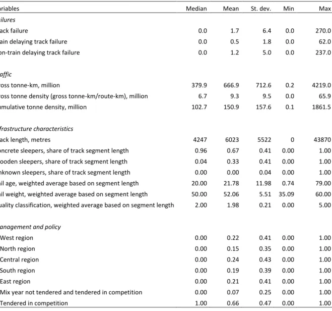
Table 2. Descriptive statistics, data per track segment and year (2003–2016), 27 012 obs.
Variables Median Mean St. dev. Min Max
Failures
Track failure 0.0 1.7 6.4 0.0 270.0
Train delaying track failure 0.0 0.5 1.8 0.0 62.0
Non-train delaying track failure 0.0 1.2 5.0 0.0 237.0
Traffic
Gross tonne-km, million 379.9 666.9 712.6 0.2 4219.0
Gross tonne density (gross tonne-km/route-km), million 6.7 9.3 9.5 0.0 65.9
Cumulative tonne density, million 102.7 150.9 157.6 0.1 1861.5
Infrastructure characteristics
Track length, metres 4247 6023 5522 0 43870
Concrete sleepers, share of track segment length 0.96 0.67 0.41 0.00 1.00
Wooden sleepers, share of track segment length 0.04 0.33 0.41 0.00 1.00
Unknown sleepers, share of track segment length 0.00 0.00 0.04 0.00 1.00
Rail age, weighted average based on segment length 20.00 21.78 11.98 0.74 79.00
Rail weight, weighted average based on segment length 50.00 52.06 5.51 35.09 60.00 Quality classification, weighted average based on segment length 2.00 1.98 0.21 0.00 5.00
Management and policy
D.West region 0.00 0.22 0.41 0.00 1.00
D.North region 0.00 0.15 0.35 0.00 1.00
D.Central region 0.00 0.24 0.43 0.00 1.00
D.South region 0.00 0.19 0.39 0.00 1.00
D.East region 0.00 0.21 0.41 0.00 1.00
D.Mix year not tendered and tendered in competition 0.00 0.07 0.25 0.00 1.00
D.Tendered in competition 1.00 0.66 0.47 0.00 1.00
The failures included in this study comprise failures on the track. Specifically, any defect on the track superstructure that is considered to be urgent (needs to be fixed immediately or within two weeks) are defined as a track failure. Switch failures are excluded from this study, considering that the age of switches often differ from the other parts of the track, which requires a separate analysis for the impact of cumulative traffic on switch failures as well as calculation of cumulative traffic on switches. Moreover, track failures caused by exogenous factors such as weather, sabotage or animals are excluded.
8 The track failures can be divided into two groups: failures that have caused train delays and failures that did not cause train delays. Evidently, the former set of failures are more urgent, requiring immediate attention so that traffic delays are minimized. The proper maintenance strategy may therefore differ between these types of failures. There is thus reason to also analyse them separately. In doing so, we need to acknowledge that the definition of a failure causing train delays has changed over the years. In years 2003 to 2010, a failure causing more than 5 minutes of delay was defined as a failure causing train delays. In year 2011, this definition changed to 3 minutes. Hence, there are failures defined as causing train delays in years 2011 to 2016 that would have been defined as a failure not causing a train delay in years 2003 to 2010. In total, failures causing between 3 to 4 minutes delay comprise between 8 to 11 per cent of all failures causing train delays per year in years 2011 to 2016. In this paper, we define these failures as failures not causing train delays.
The infrastructure characteristics considered in this study are track length, sleeper type, quality classification, rail weight, and rail age. Quality classification, rail weight and rail age vary at a more disaggregate level than the track segment level. We therefore use weighted averages (based on track lengths) of these variables in the model estimations.
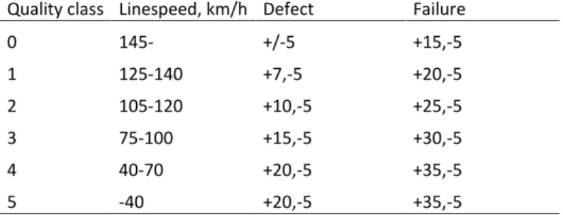
The quality classification ranges from 0 to 5, indicating high to low line speeds together with requirements on track geometry standard. Specifically, depending on the quality classification (and line speed), there are varying limits for deviations in track geometry indicating the type of maintenance activity to be carried out (or indicating the allowed deviation for newly built or renewed tracks). For example, this implies that a certain deviation can be defined as a failure on tracks with quality classification 0 (high line speed) but defined as a defect (can be rectified at a later stage) on tracks with quality classification 3 (lower line speed). An example on limits in deviations from a track gauge at 1435 mm for years 1999-2013 (a slight change is made in year 2014; see Trafikverket (2015)) is presented in Table 3.
Table 3. Limits in deviations from track gauge.
Deviation from track gauge 1435 mm Quality class Linespeed, km/h Defect Failure
0 145- +/-5 +15,-5 1 125-140 +7,-5 +20,-5 2 105-120 +10,-5 +25,-5 3 75-100 +15,-5 +30,-5 4 40-70 +20,-5 +35,-5 5 -40 +20,-5 +35,-5 Source: Trafikverket (1997)
9 4. Method
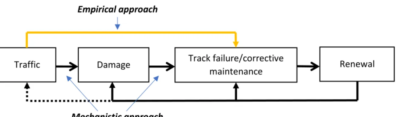
To establish a relationship between cumulative tonnes and track failures, we consider the empirical (top-down) approach in which we use observations of track failures and traffic data along with a set of control variables. An alternative is the mechanistic (bottom-up) approach that typically use simulations to predict the deterioration caused by traffic (see for example Öberg et al. (2007) who use this approach to calculate marginal costs for different vehicle types, or Smith et al. (2017) who combine the econometric and engineering approach). Figure 1 is an illustration of the approaches in the context of traffic and its relationship with track failures. The dotted line from maintenance/renewal indicates that these activities can have an impact on traffic, especially renewals that will determine the level of cumulative traffic.
Figure 1. Illustration of the empirical (top-down) and mechanistic (bottom-up) approaches in the context of traffic and track failures.
We acknowledge that both approaches have their merits and disadvantages. A strength of the empirical approach is that it uses actual frequencies of failures to establish relationships between traffic and changes in the number of failures (while controlling for confounders). A downside is that it struggles in identifying these relationships when the underlying mechanisms are complex and possibly highly correlated (and its predictive power can be questioned if there are underlying mechanisms or mediating variables that, when altered, could influence the established relationship). The mechanistic approach explicitly models these underlying mechanisms. But lack of data limits the use of this approach, and more mechanisms require more parameters that can add uncertainty to the model. Specifically, we use the empirical (top-down) approach and consider the number of track failures, 𝐹𝑖𝑡,
on track segment 𝑖 in year 𝑡 to be represented by Damage
Traffic Track failure/corrective Renewal
maintenance
Empirical approach
10 𝐹𝑖𝑡𝐽 = 𝑓(∑𝐾𝑘=1𝑄𝑘𝑖𝑡, ∑𝑚=1𝑀 𝑋𝑚𝑖𝑡, ∑𝐷𝑑=1𝑍𝑑𝑖𝑡, 𝛼𝑖), (2)
where the superscript 𝐽 indicates whether the failure caused a train delay (𝐽 = 𝐷), did not cause a train delay (𝐽 = 𝑁), or if both type of failures are included (𝐽 = 𝐵). ∑𝐾𝑘=1𝑄𝑘𝑖𝑡 is a vector of traffic variables,
∑𝑀𝑚=1𝑋𝑚𝑖𝑡 are the infrastructure characteristics and ∑𝐷𝑑=1𝑍𝑑𝑖𝑡 is a set of dummy variables such as
policy changes (introduction of competitive tendering) and year dummy variables intended to capture general trends for the entire railway network. 𝛼𝑖 is the unobserved track segment specific effect
To estimate the impact traffic has on the number of failures, we need to consider a functional form for equation 2 and choose a regression model. The distribution of failures can be of guidance in this selection (however, we base our model selection on the Akaike and Bayesian information criterions (AIC and BIC) and the estimated relationships between traffic and track failures). Figure 2 is a histogram of failures, including both failures causing train delays and other failures (𝐹𝑖𝑡𝐵). The frequency of failures
is a discrete variable (count-data) with a distribution skewed right. We therefore use count data models, namely the negative binomial and Poisson regression models. We also note that survival analysis is often used when studying track failures (see for example Lim et al. (2004), Arasteh Khouy et al. (2014), Audley and Andrews (2013)), but considering that we have multiple failures per track segment and year, we do not estimate survival models in this paper.
11 In our model specifications, the explanatory variables (except our dummy variables) are transformed with the natural logarithm. Specifically, we consider the probability of a failure, given our set of control variables and track segment specific effects (𝑃[𝐹𝑖𝑡𝐽 = 𝑓𝑖𝑡𝐽│ ∑𝐾𝑘=1𝑙𝑛𝑄𝑘𝑖𝑡, ∑𝑀𝑚=1𝑙𝑛𝑋𝑚𝑖𝑡, ∑𝐷𝑑=1𝑍𝑑𝑖𝑡, 𝛼𝑖])
where the conditional mean of our count data model is
𝐸[𝑓𝑖𝑡│ ∑𝐾𝑘=1𝑙𝑛𝑄𝑘𝑖𝑡, ∑𝑚=1𝑀 𝑙𝑛𝑋𝑚𝑖𝑡, ∑𝐷𝑑=1𝑍𝑑𝑖𝑡, 𝛼𝑖] =
𝛼𝑖𝑒𝑥𝑝 (∑𝐾𝑘=1𝛽𝑘𝑙𝑛𝑄𝑘𝑖𝑡)𝑒𝑥𝑝(∑𝑀𝑚=1𝛽𝑚𝑙𝑛𝑋𝑚𝑖𝑡)𝑒𝑥𝑝( ∑𝐷𝑑=1𝛽𝑑𝑍𝑑𝑖𝑡) (3)
where 𝛼𝑖 is the track segment specific effect. In estimating our models, we can used fixed or random
effects. The Poisson model can be estimated with conditional fixed effects. However, as stated by Allison and Waterman (2002), the conditional fixed effects negative binomial model (proposed by Hausman et al. (1984)) is not a true fixed effects estimator (indeed, time-invariant variables are not dropped when we estimate this model). We are therefore left with the random effects negative binomial model (note that using track segment dummy variables may lead to the incidental parameters problem (Neyman and Scott (1948)), which may be a problem for us considering that we have a large panel with 2129 segments in our dataset). The downside with the random effects model is that it will generate biased estimates if our regressors are correlated with the track segment specific effect 𝛼𝑖. A
solution to this problem is to use an approach proposed by Mundlak (1978), in which we add group averages of our variables (∑𝐾𝑘=1𝑙𝑛𝑄̅𝑘𝑖𝑡= 𝑇−1∑𝐾𝑘=1𝑙𝑛𝑄𝑘𝑖𝑡, ∑𝑀𝑚=1𝑙𝑛𝑋̅𝑚𝑖𝑡 =
𝑇−1∑𝑀𝑚=1𝑙𝑛𝑋𝑚𝑖𝑡, ∑𝑑=1𝐷 𝑍̅𝑑𝑖𝑡 = 𝑇−1∑𝐷𝑑=1𝑍𝑑𝑖𝑡), which means that the parameter estimates for our
time-varying versions of the variables are fixed effects (within track segment) estimates.
We include second order terms in our models. Moreover, cumulative tonnes may have an impact on track failures that vary with respect to the quality classification, or infrastructure characteristics such as rail weight, rail age and sleeper type. We therefore include interaction terms between cumulative tonnes and these variables. Specifically, we include the second order terms
1 2∑ ∑ 𝛽𝑘𝑘𝑙𝑛𝑄𝑘𝑖𝑡𝑙𝑛𝑄𝑘𝑖𝑡 𝐾 𝑘=1 𝐾 𝑘=1 , 1 2∑ ∑ 𝛽𝑚𝑚𝑙𝑛𝑋𝑚𝑖𝑡𝑙𝑛𝑋𝑚𝑖𝑡 𝑀 𝑚=1 𝑀
𝑚=1 and the interaction terms
∑𝐾𝑘=1∑𝑀𝑚=1𝛽𝑘𝑚𝑙𝑛𝑄𝑘𝑖𝑡𝑙𝑛𝑋𝑚𝑖𝑡 and ∑𝑘=1𝐾 ∑𝐷𝑑=1𝛽𝑘𝑑𝑙𝑛𝑄𝑘𝑖𝑡𝑍𝑑𝑖𝑡.
Note that the coefficients for our log-transformed variables can be interpreted as elasticities: In the count data model, we have 𝜕𝐸[𝑓|∙]𝜕𝑙𝑛𝑄 = 𝛽𝑘𝐸[𝑓| ∙], and thus, the elasticity is 𝛽𝑘 =
𝜕𝑙𝑛𝐸[𝑓|∙]
𝜕𝑙𝑛𝑄 , where we use
the fact that 𝜕𝐸[𝑓|∙]
𝜕𝑙𝑛𝑄 1 𝐸[𝑓|∙]=
𝜕𝑙𝑛𝐸[𝑓|∙]
𝜕𝑙𝑛𝑄 . With second order effects and interaction terms with other
12 𝜕𝑙𝑛𝐸[𝑓|∙] 𝜕𝑙𝑛𝑄 = 𝛽𝑘+ 2 ∙ 𝛽𝑘𝑘𝑙𝑛𝑄𝑘+ ∑ 𝛽𝑘𝑚𝑙𝑛𝑋𝑚𝑖𝑡 𝑀 𝑚=1 , (4) 5. Results
The count data models considered were the Poisson model and the negative binomial model, estimated with either fixed or random effects. The estimation results are presented in Tables 4 and 5 below and in the appendix. All estimations are carried out with Stata 12 (StataCorp.2011).
The Poisson conditional fixed effects model has a lower AIC and BIC than the negative binomial model random effects model estimated using the approach proposed by Mundlak (1978) to get fixed (within track segment) effects: 64997 and 65202 compared to 75019 and 75364 when considering all track failures. On the other hand, the Poisson random effects model has higher AIC and BIC than the negative binomial random effects model (81359 and 81613 compared to 75191 and 75453 when considering all track failures). Furthermore, the Poisson conditional fixed effects model results in failure elasticities that are decreasing with cumulative tonnes (this effect is captured by the negative coefficient for the interaction term between quality classification and a second order term for cumulative tonnes, which is -0.0891). Estimating the model with either failures causing train delays or failures not causing train delays show that it is the latter type of failures that generate this effect. Specifically, it is the track segments with quality classifications between 2 and 5 (lower line speeds and lower track standard requirements) that have downward sloping curves, while segments with a quality classification between 0 and 2 have elasticities that increase with cumulative tonnes. This relationship is also found when estimating the random effects model for failures not causing train delays, yet the decreasing relationship is less dramatic, which can explain why the random effects model with all types of failures does not indicate a downward sloping curve.3 In fact, the Poisson conditional fixed effects model
generate negative elasticities for the failures not causing train delays for a large share of segments with quality classification between 2 and 5, which is not the case for the negative binomial random effects model. Hence, we prefer the negative binomial random effects model.
3 The interaction terms between quality classification and cumulative tonnage and squared cumulative tonnage
are 0.0036 and -0.0164 in the random effects model, while the corresponding estimates are -0.0971 and -0.0891 in the fixed effects model.
13 Estimations results for all track failures are presented in section 5.1., followed by a presentation of the results for failures causing train delays and failures not causing train delays in section 5.2. Section 5.3 summarises the estimated elasticities with respect to cumulative tonnes.
5.1. Estimation results, track failures
The estimation results for the Poisson conditional fixed effects model and the negative binomial random effects model are presented in Table 4. Both models result in rather similar coefficients for most of the included variables. However, as described previously, a significant difference is that the fixed effects model generates negative elasticities for track segments with a quality classification between 2 and 5. We therefore focus on the random effect model results (despite its higher AIC and BIC), however, it should be noted that these may be biased if they correlate with unobserved track section specific effects (𝛼𝑖).
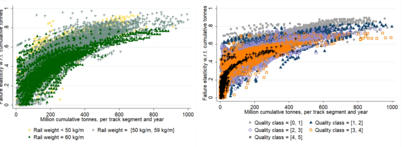
First, we can note that the first order coefficient for cumulative tonnes is 0.3858, with a second order effect at 0.1454 (both statistically significant at the 1 per cent level). This implies that the failure elasticities are increasing with cumulative tonnes, but at a decreasing rate. This is illustrated in Figures 3a and 3b below, which also show how the elasticities vary depending on the (weighted average) rail weight on segments, and their quality classifications. As shown by the interaction term between rail weight and cumulative tonnage (as well as by Figure 3a), the failure elasticity with respect to cumulative tonnage is lower for segments with heavier rails. Moreover, the segments with higher quality classifications (lower line speeds) have slightly lower failure elasticities. Recall that the differences in track standard requirements imply that a certain deviation can be defined as a failure on tracks with a low quality classification (high line speed) but defined as a defect (can be rectified at a later time) on tracks with higher quality classifications (lower line speed) (see section 3 and Table 3). Therefore, the higher elasticities for high line speeds may (partly) be explained by higher track standard requirements.
14
Table 4. Estimation results, track failures: Poisson conditional fixed effects and Negative binomial random effects.
Poisson cond. F.E. Negative Binomial R.E.
Coef. Rob. Std. Err. Coef. Std. Err.
Constant - - 0.5064*** 0.0782 ln(track length) 0.0179 0.0486 0.2396*** 0.0126 Quality class 0.0608 0.0554 0.1403*** 0.0171 ln(rail weight) -2.4008*** 0.8081 -1.8216*** 0.2070 Concrete sleeper_share -0.3684** 0.1697 -0.2986*** 0.0524 Unknown sleeper_share -0.7922** 0.3645 -0.0533 0.2324 ln(cumulative tonnes) 0.4808*** 0.1149 0.3858*** 0.0417 ln(cumulative tonnes)^2 0.1712* 0.0956 0.1454*** 0.0210
ln(rail weight)ln(cumulative tonnes) -1.5014*** 0.2946 -1.0468*** 0.1148
Quality classln(cumulative tonnes) -0.0971*** 0.0315 0.0036 0.0119
Quality classln(cumulative tonnes)^2 -0.0891*** 0.0308 -0.0164*** 0.0061
D.Mix_tendNotend 0.0309 0.0447 0.0113 0.0324 D.Tend_in_comp -0.0131 0.0501 -0.0554** 0.0275 D.North region - - -0.0140 0.0576 D.Central region - - -0.0224 0.0482 D.South region - - -0.0998* 0.0525 D.East region - - 0.3260*** 0.0503
Year dummies Yes - Yes -
Log-likelihood -32473.6 - -37563.3 -
AIC 64997.2 - 75190.7 -
BIC 65202.3 - 75453.2 -
No. of obs. 27012 - 27012 -
***, **, *: Significance at the 1%, 5%, 10% level. Continuous variables have been divided by their sample median prior to the logarithmic transformation. Thus, first order coefficients are estimates at the sample median.
The estimates show that concrete sleepers are associated with fewer track failures, the estimate being -0.2986, with standard error 0.0524 (wooden sleepers is the baseline).4 The variables for sleeper type
are expressed as share of track length and have not been log-transformed (otherwise, sections with only concrete or wooden sleepers would be lost due to its zero value). Hence, to interpret the first order coefficient, we can use ∆𝐹𝐹 = 100 ∙ [exp (𝛽̂𝑠∆𝑋𝑠) − 1], where 𝛽̂𝑠 is the parameter estimate for
variable 𝑋𝑠. This gives us the percentage change of the predicted number of failures (𝐹) when variable
4 An interaction term between sleeper type and cumulative tonnes was also tested but is not included in the final
model specifications as it to a large extent captures the impact of rail weight in the fixed effects specification (generating a negative and not statistically significant effect). Still, we can note that the coefficient is -0.1140 (standard error 0.0324) in the random effects model (and the interaction term between rail weight and cumulative tonnes changes from -1.0468 to -0.7901, both statistically significant).
15 𝑋𝑠 changes. If the share of concrete sleepers increases with 10 per cent on a track segment, the
number of track failures is expected to decrease with 100 ∙ [exp(−0.2986 ∙ 0.10) − 1] = 2.94 per cent, which implies an elasticity estimate at (-2.94/10=) -0.2942.5
Figure 3a and 3b: Track failure elasticities with respect to cumulative tonnes, per track segment and year, for different rail weights (3a, holding quality class constant) and quality classifications (3b, holding rail weight constant) (results from the negative binomial random effects estimator).
5.2 Estimation results, track failures not causing train delays and track failures causing train delays.
The track failures analysed in the previous section did not make a distinction between failures causing train delays and failures not causing train delays. Considering that the former type of failures is more urgent than the latter and may have a different relationship with traffic, we analyse them separately. The estimation results using the negative binomial random effects estimator are presented in Table 5 (see appendix for the Poisson conditional fixed effects results).
5 The elasticity varies depending on the change in variable 𝑋
𝑠 that is considered, with estimates ranging from
-0.2581 for a 100 per cent change to -0.2982 to a 1 per cent change in 𝑋𝑠 (that is, in the share of concrete
16
Table 5. Estimation results, track failures not causing train delays and track failures causing train delays: Negative Binomial random effects estimator.
Failures not causing train delays Failures causing train delays
Coef. Std. Err. Coef. Std. Err.
Constant 0.4227*** 0.0914 -0.1565 0.1159 ln(track length) 0.2392*** 0.0137 0.2238*** 0.0187 Quality class 0.1781*** 0.0205 0.2198*** 0.0242 ln(rail weight) -0.8108*** 0.2363 -0.7142*** 0.2768 Concrete sleeper_share -0.4842*** 0.0598 -0.2172*** 0.0702 Unknown sleeper_share -0.1298 0.2492 0.1480 0.4110 ln(cumulative tonnes) 0.3389*** 0.0414 0.3302*** 0.0554 ln(cumulative tonnes)^2 0.1565*** 0.0408 0.2498*** 0.0540
ln(rail weight)ln(cumulative tonnes) -1.2120*** 0.1244 -0.8168*** 0.1745
Quality classln(cumulative tonnes) -0.0193 0.0125 0.0269 0.0170
Quality classln(cumulative tonnes)^2 -0.0419*** 0.0109 -0.0438*** 0.0152
D.Mix_tendNotend -0.0048 0.0364 0.0217 0.0515 D.Tend_in_comp -0.0397 0.0307 -0.1289*** 0.0434 D.North region -0.1266** 0.0638 -0.0565 0.0745 D.Central region -0.0214 0.0530 -0.0669 0.0638 D.South region -0.0299 0.0573 -0.0084 0.0703 D.East region 0.3740*** 0.0552 0.4403*** 0.0648
Year dummies Yes Yes
Log-likelihood -31532.6 -18808.3
AIC 63129.2 37680.6
BIC 63391.0 37936.4
No. of obs. 26368 21920
***, **, *: Significance at the 1%, 5%, 10% level. Continuous variables have been divided by their sample median prior to the logarithmic transformation. Thus, first order coefficients are estimates at the sample median.
First, we note that both models have rather similar coefficients. Still, the second order effect for cumulative tonnes is smaller for failures not causing train delays, which turn out to be important for the failure elasticities for the different quality classifications: Track segments with a quality classification between 3 and 5 have failure elasticities that are decreasing with cumulative tonnes (see figure 4b).
17
Figure 4a and 4b: Elasticities for track failures not causing train delays, with respect to cumulative tonnes, for different rail weights (4a, holding quality class constant) and quality classification intervals (4b, holding rail weight constant), per track segment and year (results from the negative binomial random effects estimator).
Scatter plots of the elasticities for failures causing train delays, with respect to different rail weights and quality classifications, are presented in Figures 5a and 5b. A difference from failures not causing train delays is that there is an increasing relationship between the failure elasticities and cumulative tonnes for all quality classifications. Still, the curves indicate that the elasticities are higher for high quality classifications (low line speeds) when the track segments have low levels of cumulative tonnage (up to about 150 million cumulative tonnes), but that this relationship is reversed when the cumulative tonnage reaches around 200 million. In other words, for low levels of cumulative tonnage, a lower line speed and lower track standard requirements imply higher failure elasticities and vice versa.
18
Figure 5a and 5b: Elasticities for track failures causing train delays, with respect to cumulative tonnes, for different rail weights (5a, holding quality class constant) and quality classification intervals (5b, holding rail weight constant), per track segment and year (results from the negative binomial random effects estimator).
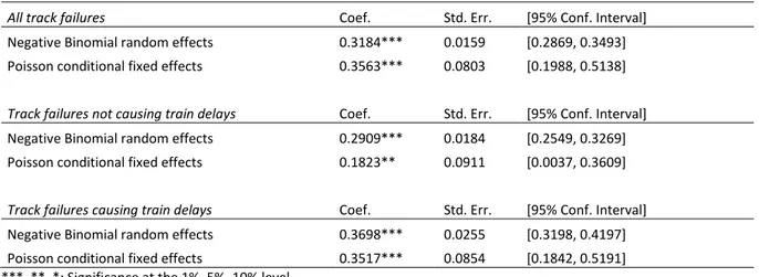
5.3 Summing up the elasticity estimates
The estimated failure elasticities with respect to cumulative tonnes are summarized in Table 6, with results from both the negative binomial random effects model and the Poisson conditional fixed effects model. There is not a big difference between the estimates from the different models, except for failures not causing train delays, where the random effect elasticity is 0.2909, while it is 0.1823 with fixed effects (however, the 95 per cent confidence intervals are overlapping).
The average elasticities differ significantly between failures not causing train delays and failure causing train delays, where the former elasticity (based on the random effects estimator) is 0.2909 and the latter is 0.3698, and the estimates have only slightly overlapping 95 per cent confidence intervals. Moreover, scatter plots of these elasticities show that their relationship with quality classification differ; the elasticities for failure not causing train delays are decreasing with cumulative tonnes for the lower line speeds, while elasticities for failure causing train delays are increasing for all quality classifications (see Figures 4b and 5b).
The elasticities for failures causing train delays are also increasing more dramatically with cumulative tonnes compared to failures not causing train delays (see Table 7 below). One reason can be that the probability of a defect becoming a failure that causes a train delay may depend on the traffic situation on the track segment. With a high traffic intensity, and failures that require long and consecutive time slots for maintenance, one could expect that the failure is more likely to lead to train delays compared to segments with low traffic intensity. This may partly explain the estimated differences between the
19 failure types, considering that the correlation coefficient between train density and cumulative tonnes is 0.70. That is, a higher level of cumulative tonnes is associated with a higher traffic intensity, which in turn is likely to imply a higher probability that a failure causes a train delay.
Table 6. Track failure elasticities with respect to cumulative tonnes.
All track failures Coef. Std. Err. [95% Conf. Interval]
Negative Binomial random effects 0.3184*** 0.0159 [0.2869, 0.3493]
Poisson conditional fixed effects 0.3563*** 0.0803 [0.1988, 0.5138]
Track failures not causing train delays Coef. Std. Err. [95% Conf. Interval]
Negative Binomial random effects 0.2909*** 0.0184 [0.2549, 0.3269]
Poisson conditional fixed effects 0.1823** 0.0911 [0.0037, 0.3609]
Track failures causing train delays Coef. Std. Err. [95% Conf. Interval]
Negative Binomial random effects 0.3698*** 0.0255 [0.3198, 0.4197]
Poisson conditional fixed effects 0.3517*** 0.0854 [0.1842, 0.5191]
***, **, *: Significance at the 1%, 5%, 10% level.
Descriptive statistics for the estimated failure elasticities with respect to different intervals of cumulative tonnes are presented in Table 7. Here it should be noted that we use elasticities that have been evaluated at the sample median of the interaction variables, that is, we exclude the impact from quality class and rail weight. Moreover, for the lowest levels of cumulative tonnes (less than 100 million tonnes), there are significant number of negative elasticities. These are also excluded in Table 7. In general, the negative binomial random effects model generates elasticities that have a smaller mean value compared to the Poisson conditional fixed effects model, except for failures not causing train delays. However, the differences in mean values between the random effects and fixed effects models are rather small in most cases.
20
Table 7. Track failure elasticities for different cumulative tonne intervals (excl. the effect of interaction terms).
All track failures Negative Binomial R.E. Poisson F.E.
Million cumulative tonnes interval Obs. Mean (std. err.) Mean (std. err.)
<100 6225a 0.2476 (0.0018) 0.3100(0.0022) [100, 200) 5879 0.4607 (0.0019) 0.5689 (0.0023) [200, 300) 3718 0.6054 (0.0013) 0.7392 (0.0016) [300, 400) 2013 0.6817 (0.0015) 0.8291 (0.0018) [400, 500) 946 0.7570 (0.0023) 0.9176 (0.0027) ≥500 1140 0.8365 (0.0022) 1.0113 (0.0026)
Track failures not causing train delays
Million cumulative tonnes interval Obs. Mean Std. Err.
<100 5301b 0.1725 (0.0013) 0.1855 (0.0011) [100, 200) 5744 0.4385 (0.0008) 0.4187 (0.0005) [200, 300) 3688 0.6068 (0.0006) 0.5243 (0.0004) [300, 400) 1992 0.7106 (0.0006) 0.5895 (0.0004) [400, 500) 939 0.7944 (0.0007) 0.6420 (0.0004) ≥500 1107 0.8969 (0.0017) 0.7064 (0.0011)
Track failures causing train delays
Million cumulative tonnes interval Obs. Mean Std. Err.
<100 2283c 0.1148 (0.0014) 0.1880 (0.0017) [100, 200) 5271 0.4042 (0.0014) 0.5341 (0.0013) [200, 300) 3440 0.6738 (0.0010) 0.8013 (0.0010) [300, 400) 1818 0.8386 (0.0010) 0.9647 (0.0009) [400, 500) 844 0.9731 (0.0011) 1.0979 (0.0011) ≥500 1051 1.1374 (0.0028) 1.2608 (0.0028)
a Negative elasticities are excluded (the Poisson model generated 6394 positive elasticities) b Negative elasticities are excluded
(the Poisson model generated 8364 positive elasticities). c Negative elasticities are excluded (the Poisson model generated
3445 positive elasticities).
6. Discussion and conclusion
In this paper, the impact of cumulative tonnes on track superstructure failures has been estimated. Failures causing train delays and failures not causing train delays are considered in the estimations, were these types of failures are added together as well as treated separately in the estimations. Specifically, the estimated track failure elasticities with respect to cumulative tonnes are increasing with the level of cumulative use, but at a decreasing rate. The effect is present for both types of failures. However, we find downward sloping curves with respect to cumulative tonnes for failures not causing train delays at track segments with lower line speeds. This relationship may be explained by an infrastructure management strategy that increases the (preventive) maintenance when track failures starts to turn up as the cumulative tonnage increases; quality issues are recognised and fixed
21 when more traffic is accumulated, thus improving their resilience against failures. Hence, this relationship can still be in line with a life cycle cost curve where maintenance costs increases with cumulative tonnes until it is beneficial to renew the asset.6 The difference between the quality classes
then suggests that the (increase in the) level of preventive maintenance when cumulative tonnage increases is relatively higher on track segments with lower line speeds, and to such an extent that the failure elasticities are decreasing with cumulative tonnes. Still, there can be other reasons for the downward sloping curves (in any case, our estimates may suffer from omitted variable bias).
One may also ask why we have certain segments with downward sloping curves for failures not causing train delays, while this is not the case for failures causing train delays. Is the latter type of failure caused by defects that are more difficult to detect (and thus prevent from becoming a train delaying failure), while the former originates from defects that are easier to spot during inspections and can be rectified before becoming a failure that causes train delays? Or are there other reasons? This is subject to future research.
Despite the differences between quality classes, the results indicate that the (average) failure elasticities are increasing with cumulative tonnes and that they vary for different track standards as measured by rail weight. The results in this paper can therefore serve as input in an economic optimization of maintenance and renewal activities. In particular, the estimated differences in the impact cumulative tonnes have on track failures with respect to different levels of cumulative use and infrastructure characteristics is useful when planning maintenance and renewal activities. For example, future research can use the results to predict the train users’ delay costs. Together with information on the impact cumulative tonnes have on track maintenance costs, the optimal timing of a track renewal can be assessed. This can improve the allocative efficiency of the infrastructure manager and, based on the current production efficiency in infrastructure provision, the results can help the government to set a proper budget constraint for rail infrastructure provision.
References
Allison, P. D., Waterman, R. P., 2002. Fixed-Effects Negative Binomial Regression Models. Sociological Methodology. 32, 247-265.
6 This suggests that we have omitted variable bias, as an increase in cumulative tonnage is expected to imply an
increase in the number of failures, ceteris paribus. We tested annual tonnage as a proxy for the maintenance activities carried out per year (especially for the number of inspections per year), but it did not change the estimated relationship.
22 Andersson, M., 2006. Marginal Cost Pricing of Railway Infrastructure Operation, Maintenance, and Renewal in Sweden: From Policy to Practice Through Existing Data. Transportation Research Record: Journal of the Transportation Research Board, No. 1943, 1-11. DOI: https://doi.org/10.3141/1943-01
Andersson, M., Björklund, G., Haraldsson, M., 2016. Marginal railway track renewal costs: A survival data approach. Transportation Research Part A: Policy and Practice, 87, 68-77. DOI: https://doi.org/10.1016/j.tra.2016.02.009
Andersson, A., Nyström, J., Odolinski, K., Wieweg, L., Wikberg, Å., 2011. Strategi för utveckling av en samhällsekonomisk analysmodell för drift, underhåll och reinvestering av väg- och järnvägsinfrastruktur. VTI rapport 706.
Andrade, A.R., Teixeira, P.F., 2011. Biobjective optimization model for maintenance and renewal decisions related to rail track geometry. Transportation Research Record: Journal of the Transportation Research Board, 2261, 163-170. DOI: https://doi.org/10.3141/2261-19
Arasteh Khouy, I., Larsson-Kråik, P-O., Nissen, A., Juntti, U., Schunnesson, H., 2014. Optimisation of track geometry inspection interval. Proceedings of the Institution of Mechanical Engineers, Part
F: Journal of Rail and Rapid Transit, 228(5), 546-556. DOI:
https://doi.org/10.1177/0954409713484711
Audley, M., Andrews, J.D., 2013. The effects of tamping on railway track geometry degradation. Proceedings of the Institution of Mechanical Engineers, Part F: Journal of Rail and Rapid Transit, 227(4), 376-391. DOI: https://doi.org/10.1177/0954409713480439
Dick, C.T., Barkan, C.P.L., Chapman, E.R., Stehly, M.P., 2003. Multivariate Statistical Model for Predicting Occurrence and Location of Broken Rails. Transportation Research Record, 1825(1), 48-55. DOI: https://doi.org/10.3141/1825-07
Gaudry, M., Lapeyre, B., Quinet, E., 2016. Infrastructure maintenance regeneration and service quality economics: A rail example. Transportation Research Part B, 86, 181-210. DOI: https://doi.org/10.1016/j.trb.2016.01.015
Hausman, J., Hall, B.H., Griliches, Z., 1984. Econometric Models for Count Data with an Application to the Patents-R & D Relationship. Econometrica. 52(4), 909-938.
Hokstad, P., Langseth, H., Lindqvist, B. H., Vatn, J., 2005. Failure modeling and maintenance optimization for a railway line. International Journal of Performability Engineering, 1(1), 51-64.
23 Jeong, D.Y., 2003. Analytical Modelling of Rail Defects and Its Applications to Rail Defect Management. U.S. Department of Transportation, Research and Special Programs Administration, Volpe National Transportation Systems Center, Cambridge, Massachusetts, January 2003.
Jiang, S., Persson, C., 2016. Malfunction in Railway System and Its Effect on Arrival Delay. In: Kumar U., Ahmadi A., Verma A., Varde P. (eds) Current Trends in Reliability, Availability, Maintainability and Safety. Lecture Notes in Mechanical Engineering. Springer, Cham. DOI: https://doi.org/10.1007/978-3-319-23597-4_18
Lim, W.L., McDowell, G.R., Collop, A.C., 2004. The application of Weibull statistics to the strength of railway ballast. Granular matter, 6(4), 229-237. DOI: https://doi.org/10.1007/s10035-004-0180-z Mundlak, Y., 1978. On the Pooling of Time Series and Cross Section Data. Econometrica. 46(1), 69-85. Neyman, J., Scott, E.L., 1948. Consistent estimation from partially con-sistent observations.
Econometrica, 16, 1-32.
Odolinski, K., 2016. The impact of cumulative tons on rail infrastructure maintenance costs. CTS Working paper 2016:28, Centre for Transport Studies, Stockholm.
Orringer, O., Tang. Y. H., Gordon, J. E., Jeong, D. Y., Morris, J. M., Perlman, A. B., 1988. Crack Propagation Life of Detail Fractures in Rails. U.S. Department of Transportation, Research and Special Programs Administration, Volpe National Transportation Systems Center, Cambridge, Massachusetts, Final Report, October 1988.
Parra, C., Crespo, A., Kristjanpoller, F., Viveros, P., 2012. Stochastic model of reliability for use in the evaluation of the economic impact of a failure using life cycle cost analysis. Case studies on the rail freight and oil industries. Proceedings of the Institution of Mechanical Engineers, Part O: Journal of Risk and Reliability. DOI: https://doi.org/10.1177/1748006X12441880
Podofillini, L., Zio, E., Vatn, J., 2006. Risk-informed optimisation of railway tracks inspection and maintenance procedures. Reliability Engineering and System Safety, 91, 20-35. DOI: https://doi.org/10.1016/j.ress.2004.11.009
Schafer, D. H., Barkan, C. P. L., 2008. A prediction model for broken rails and an analysis of their economics impact. Proceedings of the AREMA 2008 Annual Conference. Salt Lake City, Utah, United States.
Smith, A. S. J, Odolinski, K., Nia, S.H., Jönsson, P-A., Stichel, S., Iwnicki, S., Wheat P., 2016. Estimating the marginal cost of different vehicle types on rail infrastructure. CTS working paper 2016:26. Centre for Transport Studies: Stockholm.
24 Smith, A. S. J, Iwnicki, S., Kaushal, A., Odolinski, K., Wheat, P., 2017. Estimating the relative cost of track damage mechanisms: combining economic and engineering approaches. Proceedings of the Institution of Mechanical Engineers, Part F: Journal of Rail and Rapid Transit, 231(5), 620-636. Sousa, N., Alcada-Almeida, L., Coutinho-Rodrigues, J., 2018. Multi-objective model for optimizing
railway infrastructure asset renewal. Engineering optimization, DOI:
https://doi.org/10.1080/0305215X.2018.1547716
StataCorp 2011. Stata Statistical Software: Release 12. College Station, TX: StataCorp LP. Trafikanalys, 2010. Bantrafik 2009. Statistik 2010:21.
Trafikverket, 1997. Spårlägeskontroll och kvalitetsnormer – Central mätvagn STRIX. Föreskrift, BVF 587.02., 1997-08-18.
Trafikverket, 2014. BVH 524.100 – Katalog över rälsfel. TDOK 2014:0598. Version 1.0.
Trafikverket, 2015. Banöverbyggnad – Spårläge – krav vid byggande och underhåll. TDOK 2013:0347. Version 4.0.
UIC, 2002. Rail defects. UIC Code 712R. 4th edition, January 2002.
Zarembski, A.M., Einbinder, D., Attoh-Okine, N., 2016. Using multiple adaptive regression to taddress the impact of track gepometry on development of rail defects. Construction and Building Materials, 127, 546-555. DOI: https://doi.org/10.1016/j.conbuildmat.2016.10.012
Zhao, J., Chan, A.H.C., Roberts, C., Stirling, A.B., 2006. Assessing the economic life of rail using a stochastic analysis of failures. Proceedings of the Institution of Mechanical Engineers, Part F: Journal of Rail and Rapid Transit, 220(2), 103-111. DOI: https://doi.org/10.1243/09544097JRRT30 Öberg, J., E. Andersson, Gunnarsson, J. 2007. Track Access Charging with Respect to Vehicle
25 Appendix
Table 8. Estimation results, track failures not causing train delays and track failures causing train delays: Poisson conditional fixed effects estimator.
Failures not causing train delays Failures causing train delays
Coef. Rob. Std. Err. Coef. Rob. Std. Err.
ln(track length) 0.0655 0.0493 -0.0347 0.0570 Quality class 0.0527 0.0637 0.1173* 0.0700 ln(rail weight) -2.8064** 1.3344 -2.1386 1.3367 Concrete sleeper_share -0.5695*** 0.1973 -0.3031 0.2126 Unknown sleeper_share -0.9276** 0.4103 -0.8486** 0.4335 ln(cumulative tonnes) 0.3562*** 0.1213 0.4608*** 0.1355 ln(cumulative tonnes)^2 0.0982 0.0784 0.2476*** 0.0962
ln(rail weight)ln(cumulative tonnes) -2.5217*** 0.3386 -2.2924*** 0.4847
Quality classln(cumulative tonnes) -0.0953*** 0.0297 -0.0342 0.0317
Quality classln(cumulative tonnes)^2 -0.0725*** 0.0231 -0.0656** 0.0270
D.Mix_tendNotend 0.0249 0.0478 0.0739 0.0597
D.Tend_in_comp 0.0166 0.0565 -0.0456 0.0623
Year dummies Yes Yes
Log-likelihood -26383.4 -14686.1
AIC 52816.9 29422.2
BIC 53021.4 29622.1
No. of obs. 26368 21920
***, **, *: Significance at the 1%, 5%, 10% level. Continuous variables have been divided by their sample median prior to the logarithmic transformation. Thus, first order coefficients are estimates at the sample median.