2016, 2(3), 155-170
Published by the Scandinavian Society for Person-Oriented Research Freely available at http://www.person-research.org
DOI: 10.17505/jpor.2016.15
155
Local Associations in Latent Class Analysis:
Using Configural Frequency Analysis for Model Evaluation
Wolfgang Wiedermann
1and Alexander von Eye
21 University of Missouri 2 Michigan State University
Corresponding author:
Wolfgang Wiedermann, Statistics, Measurement, and Evaluation in Education, Department of Educational, School, and Counseling Psychology, College of Education, University of Missouri, 13B Hill Hall, Columbia, 65211, MO
Email: wiedermannw@missouri.edu
To cite this article:
Wiedermann, W., & von Eye, A. (2016), Local Associations in Latent Class Analysis: Using Configural Frequency Analysis for Model Evaluation Journal for Person-Oriented Research, 2(3), 155-170. DOI: 10.17505/jpor.2016.15.
Abstract
It is proposed to enrich the arsenal of methods for the evaluation of local independence within latent classes by methods from Configural Frequency Analysis (CFA). CFA provides researchers with two additional options. The first involves identifying those patterns of categories of manifest variables that contradict the assumption of local independence within a given class. If such patterns exist, local independence is viewed as violated not (only) at the level of relations among variables, but at the level of individual patterns that occur at rates significantly different than expected under the assumption of variable inde-pendence. The second option involves comparing classes at the level of individual patterns. The results of such a comparison of classes can be that outlying patterns are identified as class-specific. Second, it is possible that classes differ in the occur-rence rates of individual patterns (i.e., specific response patterns may be more likely to occur in certain classes). This can occur even when these patterns do not contradict the assumption of local independence. An empirical example is given using data on alcohol consumption behavior among college students. Extensions and applications of the proposed methods are discussed.
Keywords: Latent Class Analysis, Conditional Independence, Local Association, Configural Frequency Analysis
The modern person-oriented approach (cf. Bergman & Magnusson 1997; Bergman, von Eye & Magnusson, 2006; von Eye, Bergman, & Hsieh, 2015) considers the individual as a functioning totality and identifies individual patterns of information as the conceptual and analytic units (known as “pattern summary”). Prototypical patterns are assumed to occur frequently in practice and, thus, a small number of patterns may be sufficient to explain variation in empirical data (so-called “pattern parsimony”). In cross-sectional data settings, various statistical methods, such as cluster analysis, latent class analysis, latent profile analysis, and configural frequency analysis, have been called ideal-ly-suited to test person-oriented hypotheses. Latent class
analysis (LCA) has become the standard tool for mod-el-based classifications of observed categorical data.
The appropriateness of latent class models is usually evaluated using overall goodness-of-fit measures such as information indices, e.g., the Akaike information criterion (AIC), the Bayesian Information Criterion (BIC), and their derivatives, dissimilarity indices, or goodness-of-fit statis-tics such as the likelihood ratio statistic (see Morgan, 2015). In this article, we add to the arsenal of evaluation tech-niques Configural Frequency Analysis (CFA). CFA consti-tutes one of the main methods of person-oriented research (cf. Bergman, Magnusson & El-Khouri, 2003). The method allows one to identify the location of deviations from local
156 independence, that is, class-specific individual cells that contain numbers of cases that deviate from expectation. In addition, this method allows one to test specific hypotheses about the presence or absence of local independence in particular sectors of the class-specific data space. CFA can be applied when evaluating individual classes and when comparing classes. Both options are discussed in this article which is structured as follows. First, we review LCA and CFA. We then discuss methods of evaluation of LCA mod-els, and embed CFA into the canon of these methods. Third, we present two examples of latent class model evaluation using CFA in analyzing alcohol consumption patterns among young adults.
Latent Class Analysis
LCA, originally proposed by Lazarsfeld and Henry (1968; cf. Clogg, 1995; Goodman, 1974; Rindskopf, 1990; Vermunt, 1997), is a member of the general class of latent structure models. This class also includes factor analysis models, covariance structure models, latent profile models, latent trait models, and models used in Item Response The-ory (IRT). LCA uses categorical manifest variables to cre-ate ccre-ategorical lcre-atent variables (see Bartholomew & Knott, 1999, Table 1.1). Individual cases, all with class member-ship unknown prior to analysis, can be assigned to the classes of the latent variables.
The LCA Model
Using the formulation by Lazarsfeld and Henry (1968), the unrestricted latent class model for one latent variable can be described as
j g Y g Y Y Y G,1, 2,3,... j| ,where G denotes the latent variable, the Ys denote the man-ifest variables, πg is the latent probability of Class g, and
the conditional probabilities πYj|g (j = 1, …, k; with k
denot-ing the number of manifest variables) are called conditional
response probabilities. Parameters are estimated by means
of the expectation-maximization (EM) algorithm (Dempster, Laird & Rubin, 1977). The model equation implies that, within each latent class, the manifest variables are assumed to be independent from each other, thus reflecting the as-sumption of local independence (cf. the Axiom of local independence; see Clogg, 1995). If this assumption is met, the manifest variables should be independent of each other in each of the latent classes or, in more technical terms, the model of variable independence should prevail in each of the latent classes. Later, in this article, we will discuss CFA as a method that can be used to test this assumption.
Haberman (1979) showed that the unrestricted LCA model can equivalently be expressed as a log-linear model. For the model specified above, one obtains
i i Y G gj Y j G g j i g i im
,, ,... ,log
.This is a model for the G×Y1×Y2 ×Y3… cross-classification.
The latent variable, G, is unknown a priori. Therefore, this cross-classification is incomplete. Zero-sum restrictions are imposed on all parameters for identification purposes.
Measuring Fit
The expected frequencies are obtained as
,... , , ,... , ,
ˆ
gi jn
gi jm
.These values can be compared with the observed frequen-cies, mg,i,j,…. Usually, researchers employ, for this
compar-ison, members of the Cressie-Read power divergence fam-ily, e.g., the Pearson goodness-of-fit statistic
l l l lm
m
m
ˆ
)
ˆ
(
2 2 ,where l goes over all cells of the cross-classification, or the likelihood ratio statistic
l l l lm
m
m
LR
ˆ
log
2
2 ,for ml > 0. Remember that programmers keep the
conven-tion that log(0) = 0; this has the effect that cells with m = 0 will not prevent LR χ2 from being calculated, and that χ2
and LR χ2 are, occasionally, far from one another. Because
asymptotic conditions for these χ2 statistics may not be met
for sparse cross-tables, large deviations of LR χ2 and
Pear-son’s χ2 statistic are indicative for biased p-values. In these
cases, several authors suggested to use parametric boot-strapping techniques (e.g., Agresti, 1992; Collins at al., 1993; von Davier, 1997).
A number of fit statistics is not directly linked to the χ2
distribution. Examples include the index of dissimilarity and information criteria. Methods to assess local fit of a latent class model (see Garrett & Zeger, 2000; Hagenaars, 1988; Vermunt & Magidson, 2000) are typically based on the comparison of pairwise observed and model-predicted cross-classification frequencies. Higher association of pairwise items in the observed 2 × 2 table than in the ex-pected 2 × 2 table is indicative for violations of the condi-tional independence assumption. Qu, Tan, and Kutner (1996) considered continuous latent variables in an attempt to assess residual correlations (for a generalization, see Uebersax, 1999; for a discussion of this generalization in relation of multiple latent classes and the need to consider multiple residual correlations, see Aspahourov & Muthén, 2015).
Practically, all of these statistics are overall measures. That is, they represent the entire cross-table. The added correlations between manifest variables and the residual
157 correlations, both discussed by Aspahourov and Muthén (2015), are estimated based on the entire range of possible scores of the indicator variables. In the present article, we propose also looking at individual cells of the cross-classification of the manifest and the latent variables (see also Maydeu-Olivares & Liu, 2015). Specifically, we present CFA as a method that allows one to inspect indi-vidual cells or groups of cells, and we focus on statistics that are linked to some sampling distribution.
Configural Frequency Analysis
CFA (Lienert, 1968; von Eye, 2002; von Eye & Gutiér-rez-Peña, 2004; von Eye, Mair, & Mun, 2010) allows re-searchers to determine whether an individual cell in a cross-classification comes with an observed frequency that is discrepant from the frequency that was expected for this cell. Specifically, consider Cell l for which a researcher asks whether the difference between ml and is
signifi-cant. The null hypothesis under which this question is an-swered is where, as in the last section, l goes over all cells of the cross-classification, E[ml] is the
expectancy for Cell l, and is the expected frequency for Cell l under a base model (see von Eye & Gutiérrez-Peña, 2004; von Eye & Mun, 2016). A first reason for this null hypothesis to be rejected is that Cell l constitutes a CFA
Type. In this case, it is rejected because the binomial
proba-bility of an observed cell frequency, given the sample size n, is
(
1
)
1
, l nm
B
l ,where πl is the probability of Cell l and α is the nominal
significance level (e.g., 5%). In words, Cell l constitutes a CFA Type if it contains more cases than expected. In the second case, the null hypothesis is rejected because Cell l constitutes a CFA Antitype. In this case, it is rejected be-cause
(
)
, l nm
B
l .In words, Cell l constitutes a CFA Antitype because it con-tains fewer cases than expected. In the third case, the null hypothesis prevails because the number of observations in Cell l is consistent with the base model.
CFA Tests for Individual Configurations
A large number of tests has been proposed for CFA. Here, we focus on two tests (for more detail and more tests, see Lehmacher, 1981; von Eye & Mair, 2008; von Eye, 2002). The first test to be described here is the binomial test. It can be employed under any sampling scheme (multinomial, product-multinomial sampling). Given ml, the exact tail
probability of ml and more extreme frequencies is
e a j j n j l lp
q
j
n
m
B
(
)
, Where q = 1 – p, a = 0 if and a = ml if , e = ml if a = 0, and e = n if a = ml. Unless it isknown a priori, the value of p is estimated from the sample. The binomial test is exact. Given the base model (to be explained below), the probability of each frequency is cal-culated and added to the total. The binomial test is recom-mended in particular when a sample is so small that the approximation properties of approximate tests are doubtful.
The second test to be reviewed here is the z-test. Com-parisons with other CFA tests suggest that the z-test has desirable properties (in terms of statistical power and Type I Error robustness) even under adverse conditions (see von Weber, von Eye, & Lautsch, 2005). It is
npq
np
m
z
l
,with z approximating the standard normal distribution. The
z-test can also be applied under any sampling scheme.
The CFA Base Model
CFA base models are probability models in which re-searchers specify variable relations and other effects. Emergence and interpretation of CFA Types and Antitypes vary with these specifications (Mellenberg, 1996). Most base models can be expressed as log-linear models, but there are exceptions such as the model of axial symmetry or the model of point symmetry (von Eye, 2002). In this arti-cle, we focus on models that can be expressed as log-linear models.
CFA base models have three main characteristics (von Eye, 1988, 2004):
1. they represent theoretical assumptions concerning the nature of the variables as either of equal status or members of groups such as predictors, media-tors, or criteria;
2. they consider the sampling scheme under which the data were collected; and
3. they include in the model specification all effects the researchers are not interested in.
In the present context, the third of these characteristics is most important. We illustrate this characteristic using two base models. Specifically, these are the model of first-order CFA and the model for two-group CFA. To illustrate the first-order base model – this is the one that was originally proposed for use in CFA (Lienert, 1968) –, we use the four variables Y1, Y2, Y3, and Y4. The base model is that of
varia-ble independence. All it contains is the variavaria-bles’ main ef-fects. It can be written as
158 4 3 2 1
log
m
Y
Y
Y
Y ,where the superscripts indicate that the effects of individual variables are included, that is, the main effects. When this model is rejected, variable interactions must exist, and re-searchers have two options. One option is to identify the interactions that exist in the space of the variables included in the model. Pursuing this option is routine in log-linear modeling. The other option is to identify those cells that reflect particularly strong or significant deviations from the base model, in the form of Types or Antitypes. These cells show where, in the cross-classification, “the action is.” The second option is pursued when CFA is applied (von Eye & Gutiérrez-Peña, 2004). The base model of first-order CFA can be extended by also considering all two-way interactions (2nd order CFA), all three-way interactions (3rd order CFA)
etc., or by including covariates or special effects. The search for important variable interactions is routinely performed in
variable-oriented research. The search for outstanding cells
is usually performed in person-oriented research (see Bergman & Magnusson, 1997; von Eye & Bergman, 2003; von Eye, Bergman, & Hsieh, 2015). Naturally, these two lines of research can be pursued in tandem.
To illustrate the base model for two-group CFA, consider the variables G, Y1, Y2, and Y3, where G is the grouping
variable and the Y variables are used to discriminate between the two groups. The base model for this analysis is
,
log
3 2 1 3 2 3 1 2 1 3 2 1 Y Y Y Y Y Y Y Y Y Y Y Y Gm
where the double-superscripted terms indicate two-way interactions, and the triple superscripted term indicates the three-way interaction among all three discrimination varia-bles (Y1, Y2, and Y3). This model can be rejected only if
interactions between the grouping variable, G, and combi-nations of the discrimination variables exist, that is, when the groups differ in the sub-tables spanned by the discrimi-nation variables. This model is saturated in the discrimina-tion variables. The interacdiscrimina-tions among the discriminadiscrimina-tion variables must not be the reasons why the model fails, and thus reflect the third of the above characteristics of CFA base models.
The two-group CFA base model can also be extended, for example, by increasing the number of groups or the number of grouping variables, or by also including covariates or special effects. The relations of this model to the log-linear model for logit analysis have been discussed by von Eye, Mair, and Bogat (2005).
Protection of the Nominal Significance Level α
In practically all applications of CFA, exploratory and confirmatory, the observed frequencies in multiple cells are subjected to a CFA test. It has been shown that, depending on the size of the table, these tests are, to a certain degree,
dependent upon each other. One extreme is that the tests are completely dependent. When a 2 × 2 table is examined under the base model of first-order CFA, only the result of the first test is open. The following three tests are completely de-termined (von Weber, Lautsch, & von Eye, 2003). As the size of a table increases, the degree of dependence decreases, but CFA tests are never fully independent (Krauth, 2003; von Eye et al, 2010).
Methods of protection of the nominal significance level α take this dependence into consideration, to various degrees. The best known method, Bonferroni protection, only con-siders the total number of tests. Positing that the α level be the same for each test, the protected α threshold is α* = α/h,
where h indicates the total number of tests, usually the size of the table. Relaxing the requirement that the α level be the same for each tests, Holm (1979) proposes taking into con-sideration both the total number of tests and the number of tests already performed before the current, the ith test. The resulting protected threshold then is
1
*
i
h
,where i is the rank of the size of the residual under test, in descending order. Holm's α protection suggests less con-servative statistical decisions than the Bonferroni procedure. Even less conservative decisions are suggested by Holland and Copenhaver's procedure (1987). The authors propose, for the ith test,
1 1 *
)
1
(
1
h i .This procedure is clearly less restrictive than the Bonferroni protection. It is also (slightly) less restrictive than Holm's (1979) procedure (for comparisons of procedures for the protection of α, see Olejnik, Li, Supattathum, and Huberty, 1997; von Eye, 2002).
Specifically developed for use in CFA are the α protection procedures by Hommel, Lehmacher, and Perli (1985; cf. Hommel, 1988, 1989). Proposing modifications of Holm's procedure that can be used when two- and three-dimensional tables are explored, these authors use the result that, under certain conditions, the hypotheses tested in single cells can be viewed as intersections of a number of other hypotheses. Therefore, in a sequence of CFA tests, a certain number of tests can be performed at the same protected α level. By implication, this level is less restrictive than the one result-ing from the original Holm procedure. The Hommel et al. (1985) procedure that results, for instance, for a table of size 3 × 3 or larger leads to the following values of protected αs:
159
.
,
2
,
7
,
6
,
4
...
,
/
* * 1 * 8 * 7 * 6 * 5 * 2 * 1
h hh
h
h
h
As for the procedures by Holm (1979) and Holland and Copenhaver (1987), the test statistics must be ranked in descending order before the tests are performed. In all pro-cedures that require ranking of test statistics, the procedure concludes as soon as the first null hypothesis prevails.
Using CFA to Test Local Associations in
LCA
We now discuss the application of CFA in the examination of local independence in latent classes. As was mentioned above, three groups of tests are generally used to evaluate local independence. These groups differ in the amount of information they use in each particular test. The first group uses global tests. It includes overall goodness-of-fit tests such as the Pearson χ2-test or the LR χ2-test. The well-known
information criteria (such as AIC, cAIC, BIC, or adjusted BIC) are also members of the group of overall model eval-uation, and so is the measure of dissimilarity. In the second group, we find tests that allow one to compare pairs of items or questions. Members of this group include χ2-tests and the
odds ratio. Methods for discovering residual associations between the manifest variables in LCA have been proposed by Aspahourov and Muthén (2015). In the third group, in-dividual residuals are used. Examples of measures in this group include the Pearson χ2-component and the
standard-ized residual. Any other residual measure could be used as well.
Here, we propose using the arsenal of CFA methods to test hypotheses that are compatible with local independence. To define local independence, we use concepts and definitions that are discussed in test theory and LCA. In classical test theory (Lord & Novick, 1968), local uncorrelatedness (see also Su & Ullah, 2009) is among the key characteristics of a psychometric test. When this characteristic obtains, a tes-tee’s responses to test items are uncorrelated. Violations have the effect that the equations become invalid that are generally used to establish psychometric properties of a test. In probabilistic test theory or IRT, items must be locally
independent. This implies that not only linear relations, as
they are assessed using measures of correlation, but also any other form of dependence must not exist. This definition is also used in LCA.
More specifically, items show local stochastic
independ-ence, if
j j kg
P
Y
g
Y
Y
P
[(
11
)
...
(
1
)
|
]
(
1
|
)
,where P(Yj = 1) indicates the probability that Item j (j = 1, …,
k) in Class g is responded to in the affirmative. This applies
accordingly when items have more than two response cat-egories. In LCA, stochastic independence is the goal of analysis in every class. This implies, in the present context, that the latent class solution accounts for item associations in every class, and items are unrelated to each other. We now propose two CFA models that can be of use when local independence is tested. The first model is applied to each latent class. The second model serves to compare two or more latent classes.
Local Independence in a Latent Class
From a log-linear perspective, the above definition of local independence implies that the items are independent. When local independence exists, the log-linear main effect model will prevail, that is, the model
k Y Y Y j
m
...
log
1 2 ,where j indexes the variables again and k is the number of items. This is also the model of first-order CFA that was introduced above. Here, we propose employing first-order CFA to evaluate local independence in each class.
Using first-order CFA to evaluate local independence comes with all the benefits that come with CFA. These benefits include
1. There is an overall Pearson χ2- or likelihood ratio
χ2-test that is equivalent to the tests reported for LCA;
2. cell-specific deviations can be significant even when the overall test suggests variable independence; 3. there exists a large number of tests for individual cells
that allow researchers to either explore the entire cross-classification of items for one latent class, or test specific hypotheses for a latent class; either approach can result in CFA Types and Antitypes that indicate which item category combinations – the CFA
configu-rations – represent deviations from local
independ-ence;
4. hypotheses can be tested that concern groups of item combinations; examples of such hypotheses can target sequences of responses or response patterns;
5. covariates can be taken into account that may help ex-plain the existence of CFA Types or Antitypes, that is, local deviations from independence;
160 6. well-developed procedures for the protection of α exist
within the CFA framework that adjust the significance threshold based on the number of tests performed; ap-plication of these procedures can help answer ques-tions of how to take into account the possible depend-ence of tests, questions that were asked repeatedly in user forums (and met, in some instances, with answers that did not consider this form of dependence; see, e.g., http://www.statmodel.com/discussion/messages/13/38 95.html)
7. the postulate of local independence can be relaxed by including local associations in the CFA base model; local associations can be more parsimonious than standard associations because they involve selections of variable categories instead of all variable categories.
Comparing Latent Classes With Respect to
Local Independence
The null hypothesis of equivalence of local
independ-ence posits that classes do not differ in local independindepend-ence.
Alternatively, items can behave differently across classes even when, for each class, the model of independence pre-vails. To identify such items, we propose a new base model for multiple-group CFA. The base model for standard mul-tiple group CFA contains at least one variable that indexes the groups (the latent classes), and at least one variable that is used to discriminate between the groups (von Eye, 2002). The base model for standard multiple group CFA is set up as a hierarchical log-linear model with the following char-acteristics:
1. it contains all possible effects of the discrimination variables; it is, thus, saturated in the discrimination variables; the reason for this specification is that rela-tions among the discrimination variables must not be causes for Types and Antitypes to emerge;
2. it contains the main effect of the variables that indexes the groups; if there is more than one grouping variable, the model must be saturated in these variables as well, for the same reason it is saturated in the discrimination variables;
3. it posits independence of grouping from discrimination variables.
If this model fails, researchers know that the hypothesis of equivalence of local independence is violated, in general. In addition, Types and Antitypes can be expected to emerge. They indicate where local associations are between the classification variable(s) and the discrimination variables.
In the context of testing equivalence of local independ-ence, these Types and Antitypes indicate where, in the cross-classification, grouping and discrimination variables are locally associated in the sense that latent classes differ from each other. Phrased differently, and following the definition of a CFA base model that was given above, we
first specify the effects in the cross-classification of the grouping with the discrimination variables that we are not interested in:
1. all main effects;
2. all interactions among the discrimination variables; these effects – if they exist – must not be causes for Types and Antitypes to emerge, because they do not speak to the null hypothesis tested in the present con-text; when conditional independence exists within each of the comparison groups, the parsimony principle (Wu & Hamada, 2009) can be utilized, and these in-teractions can be omitted from the model;
3. all three- and higher-way interactions among the grouping and the discrimination variables; if these in-teractions exist, they suggest that the grouping variable qualifies the two- or higher-way interactions among the discrimination variables; as before, when condi-tional independence exists, these interactions can be omitted from the model.
What remains are the two-way interactions between the discrimination variables and the grouping variable. When these effects exist, the main effects that are the sole effects that may exist when local independence prevails, differ across the comparison groups, that is, the latent classes. In the present context of testing hypotheses that are compati-ble with local independence, these are the effects we are interested in. In a CFA base model, these are, therefore, the only effects to be left out. When Types or Antitypes emerge, they indicate where in the table latent classes differ in local independence characteristics.
To illustrate, consider the grouping variable, G, and the three discrimination variables Y1, Y2, and Y3. For these four
variables, we present three possible CFA base models. First-order CFA of the cross-classification of these four variables, that is,
3 2 1
log
m
G
Y
Y
Y ,shows where in the table deviations from independence exist. If they exist, they could be indicative of differences in local independence. However, they could also simply be indica-tive of associations among the discrimination variables. Therefore, this model is, under most conditions, not in-formative for decisions concerning the hypothesis of dif-ferences in local independence.
The model 3 2 1 3 2 3 1 2 1 3 2 1
log
Y Y Y Y Y Y Y Y Y Y Y Y Gm
is the base model of standard multiple-group CFA. When this model fails, the comparison groups differ in the dis-crimination variables (see von Eye & Mun, 2013).
161 The model G Y Y Y G Y Y G Y Y G Y Y Y Y Y Y Y Y Y Y Y Y Y Y G
m
3 2 1 3 2 3 1 2 1 3 2 1 3 2 3 1 2 1 3 2 1log
is the new multiple group base model that we propose for testing hypotheses concerning or exploring local inde-pendence in the comparison of two or more groups. The only terms not included in this model are the two-way interac-tions between the grouping and the discrimination variables.
Data Example: Alcohol Consumption
Patterns Among Students
The following data example describes results from a survey concerning alcohol consumption behavior among Austrian university students. Overall, 1839 students (56.8% female; average age: 26.3, SD = 10.0) provided data on the Alcohol Use Disorder Identification Test (AUDIT; Saunders & Aasland, 1987) which is a widely used questionnaire to measure hazardous drinking patterns. The AUDIT com-prises 10 items addressing alcohol consumption and alco-hol-related negative consequences. For the present purpose, we dichotomized the scores of each item following Smith and Shevlin (2003): The baseline category reflects answers scoring zero on the scale (e.g., reflecting the response option “never” for questions like “How often do you have six or more drinks on one occasion”). The second category re-flected all remaining response options on the scale. We analyzed the following 6 items: A2 (“Typical amount of alcohol on a drinking day”), A3 (“How often 6+ drinks on one occasion”), A4 (“Unable to stop once started drinking”),
A5 (“Failed to do what was expected due to drinking”), A7
(“Guilt after drinking”), and A8 (“Memory loss”).
The question we ask is whether latent classes can be identified that capture the unmeasured heterogeneity in the participants’ responses to questions on drinking behavior. This effort is meaningful in particular when variables are related to each other and when respondents are assumed to reflect heterogeneous drinking behavior patterns. Before performing an LCA, we, therefore first performed a CFA using the data from the complete sample. Specifically, we performed a first-order CFA under the base model
8 7 5 4 3 2
log
m
A
A
A
A
A
A where the superscripts indicate the questionnaire items used in the present analyses. For the CFA, we used the z-test described above. Table 1 summarizes the results of this CFA in terms of Types and Antitypes.The overall goodness-of-fit of the main effect model is deplorable. We obtain the Pearson χ2 = 4,571.868, LR χ2 =
2,022.773, Raftery’s BIC = 1,599.800, and a dissimilarity index of 37.015. For df = 57, both χ2 measures suggest
re-jecting the model (p < 0.01). From a CFA perspective, we
note that a large number of configurations deviates from expectancy, most notably the first (all answers negative), and the last (all answers affirmative). For both of these configurations, significantly more cases were observed than expected under the assumption of item independence. We conclude that strong variable associations exist.
Latent Class Models
To answer the question whether there are groups of indi-viduals with specific response patterns, we performed a series of latent class models using Mplus (Muthén & Muthén, 2015). The AIC (Akaike, 1987), the BIC (Schwarz, 1978) and the sample size adjusted BIC (Scolve, 1987) were used to decide upon the number of latent classes (lower values indicate a better fit of the model). Nylund, As-parouhov, and Muthén (2007) showed that the AIC tends to overestimate the correct number of latent classes. Thus, we rather focused on BIC- and adjusted BIC-values for model selection. In addition, the unadjusted and adjusted Lo-Mendell-Rubin test (Lo, Mendell, & Rubin, 2001) was applied to assess whether the g class solution is superior to the g – 1 class solution. A non-significant test result suggests no superiority of the g class solution over the g – 1 class model. Entropy and the average profile probabilities were inspected to assess classification uncertainty of each latent class solution. As suggested by Marsh, Lüdtke, Trautwein, and Morin (2009) interpretability of model coefficients was inspected for each solution. Models were estimated using 1000 random starts. Table 2 summarizes the model fit indi-ces for g = 2, …, 6 latent classes. Overall, the BIC, the ad-justed BIC, the LMR-test, as well as the adad-justed LMR-test favored the 4-class solution. The AIC favored the 5-class solution. Entropy measures were rather low ranging from 0.643 to 0.733. Pearson and LR χ2-tests rejected the null
hypothesis of model fit for each LC model. Based on the model goodness-of-fit measures (taking into account the interpretability of estimated parameters) the decision was to retain the 4-class solution.
Figure 1 shows the four latent classes representing typical alcohol consumption patterns of the 1831 respondents. The most prevalent group is Latent Class 1 (38.4%) and is characterized by high probabilities of having more than 1 or 2 alcoholic drinks on a typical drinking day, engaging into binge drinking at least monthly, and experiencing rather mild negative consequences. The second largest class (La-tent Class 3; 31.7%) shows rather low probabilities on all items reflecting very mild alcohol consumption with no negative consequences. Latent Class 4 (24.1%) shows the most severe consumption pattern with rather high probabil-ities on all items reflecting heavy alcohol use and experi-encing multiple negative consequences. Finally, Latent Class 2 (5.8%) constitutes the smallest class with moder-ately high probabilities on all items, representing moderate alcohol consumption with moderately negative conse-quences.
162
Table 1. Types and Antitypes from first-order CFA (complete study sample).
Configurations A2 A3 A4 A5 A7 A8 n expected z p-value CFA Decision 0 0 0 0 0 0 288 35.30 42.53 <.001 Type 0 0 0 0 0 1 6 22.50 –3.48 <.001 Antitype 0 1 0 0 0 1 17 51.60 –4.82 <.001 Antitype 0 1 0 0 1 0 12 37.75 –4.19 <.001 Antitype 0 1 0 0 1 1 4 24.06 –4.09 <.001 Antitype 0 1 0 1 0 0 22 47.45 –3.69 <.001 Antitype 0 1 0 1 0 1 9 30.24 –3.86 <.001 Antitype 0 1 1 0 0 1 4 17.17 –3.18 0.001 Antitype 0 1 1 1 0 0 1 15.79 –3.72 <.001 Antitype 1 0 0 0 0 0 92 64.62 3.41 <.001 Type 1 0 0 0 0 1 10 41.18 –4.86 <.001 Antitype 1 0 0 0 1 1 0 19.20 –4.38 <.001 Antitype 1 0 0 1 0 0 9 37.86 –4.69 <.001 Antitype 1 0 0 1 0 1 3 24.13 –4.30 <.001 Antitype 1 0 0 1 1 0 2 17.65 –3.73 <.001 Antitype 1 0 1 0 0 0 3 21.51 –3.99 <.001 Antitype 1 0 1 0 0 1 1 13.70 –3.43 <.001 Antitype 1 0 1 0 1 0 0 10.03 –3.17 0.001 Antitype 1 1 0 0 0 0 190 148.23 3.43 <.001 Type 1 1 0 0 1 0 38 69.10 –3.74 <.001 Antitype 1 1 0 1 0 0 54 86.85 –3.53 <.001 Antitype 1 1 0 1 0 1 92 55.35 4.93 <.001 Type 1 1 0 1 1 1 65 25.80 7.72 <.001 Type 1 1 1 0 0 0 18 49.33 –4.46 <.001 Antitype 1 1 1 0 1 1 33 14.66 4.79 <.001 Type 1 1 1 1 0 1 52 18.42 7.82 <.001 Type 1 1 1 1 1 1 144 8.59 46.21 <.001 Type
Table 2. Goodness-of-fit of various LC models (AIC = Akaike Information Criterion, BIC = Bayes Information Criterion,
adj. BIC = adjusted BIC, LMR = Lo-Mendell-Rubin test; minimum values for the information criteria are marked italic).
Pearson
No. of
classes AIC BIC adj. BIC χ2 (df) p-value Entropy
p-value LMR p-value adj. LMR 2 11684.8 11756.4 11715.1 384.5 (50) <.001 0.733 < .001 < .001 3 11488.0 11598.2 11534.7 159.5 (43) <.001 0.650 < .001 < .001 4 11446.3 11595.1 11509.3 65.1 (36) <.001 0.643 0.001 0.001 5 11443.3 11630.7 11522.7 49.4 (29) 0.011 0.685 0.405 0.411 6 11445.2 11671.2 11540.9 34.7 (22) 0.042 0.645 0.453 0.457
163
Figure 1. Latent class profiles based on the 4-class solution [□ = LC1 (38.4%), ■ = LC2 (5.8%), ● = LC3 (31.7%), ○ = LC4
(24.1%)]
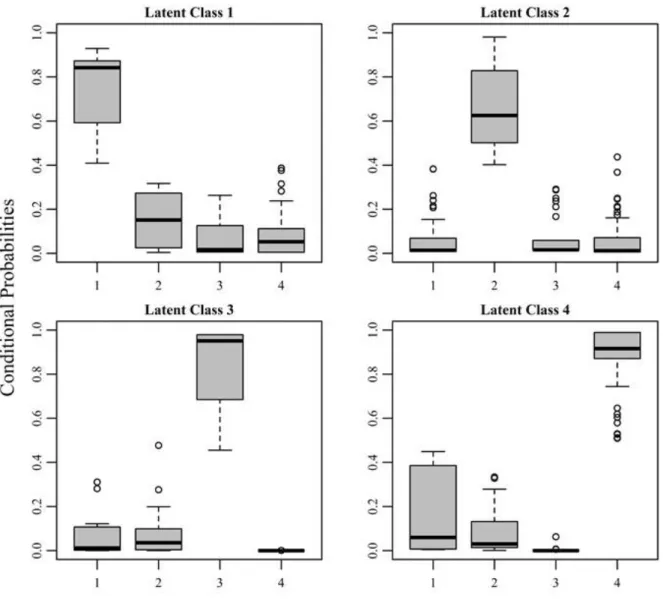
Evaluating bivariate χ2 goodness of fit statistics showed a
largest z-value of 2.902 for items A5 (“Failed to do what was expected due to drinking”) and A8 (“Memory loss”) sug-gesting non-independence of the two indicators (all re-maining z-values ranged from 0.000 to 1.579). Further, to informally assess the classification uncertainty of latent classes, Figure 2 gives the boxplot of estimated conditional probabilities for the latent classes. Latent Class 2 (“moderate alcohol consumption with moderate negative consequences”) showed the lowest conditional probabilities (see upper right panel of Figure 2). Further, respondents who were assigned to Latent Class 1, showed also relatively high conditional probabilities for Latent Class 2 (upper left panel of Figure 2). Similarly, respondents assigned to Latent Class 4 showed comparatively large conditional probabilities for Latent Class 1. Overall, latent classes were most distinct in case of membership of Latent Class 3.
Local Independence in Individual Classes
In a first series of analyses, we pursue the question whether, in each of the four classes, local independence exists. To answer this question, we first estimated, for each class, the log-linear main effect model specified above, and then per-formed the CFA tests. The second analysis was conducted to identify class-specific locations of violations of local inde-pendence. CFA tests were performed only when, overall, the null hypothesis of local independence was rejected.
Based on the overall goodness-of-fit χ2-tests, the null
hypothesis of local independence was violated in three of the four latent classes, Class 3 being the only exception. For Class 1, for example, we obtained the Pearson χ2 = 191.719,
LR χ2 = 223.404, Raftery’s BIC = –144.542, and a
dissimi-larity index of 19.583. For df = 57, the two χ2 measures
suggest rejecting the model (p < 0.01), and we have reason to expect that CFA Types and Antitypes emerge. We, there-fore, performed a CFA under the same specifications as for Table 1.
164
Figure 2. Boxplots of estimated conditional probabilities of latent class membership.
Figure 3 gives the z-approximated CFA test statistic of response patterns for the Latent Classes 1, 2, and 4. Hori-zontal solid lines refer to the Bonferroni-corrected z-value reflecting the nominal significance level of 5% (based on 65 tests we arrive at α* = .05/65 = .00008 which corresponds to
the zadj = 3.36). Thus, z-statistics larger than 3.36 correspond
to CFA Types, and z-statistics smaller than –3.36 indicate CFA Antitypes. In this data set, Antitypes are more prevalent than Types and are particularly common for patterns indi-cating less harmful alcohol use/consequences in Latent Classes 1 and 4 reflecting heavy alcohol consumption pat-terns. In Latent Class 1 (“heavy consumption with mild negative consequences”), CFA Types are constituted by Configurations 1 1 1 0 0 0 (n = 18, i.e., 2.5% of class members and 0 1 0 1 0 0 (n = 22, 3.1%). Both configurations
reflect characteristic patterns for this class indicating 1) heavy alcohol consumption including binge drinking events while feeling unable to stop drinking and 2) binge drinking occasions together with a higher risk of failing to do what was expected due to drinking. Thus, based on the charac-teristics of both CFA Types, we can conclude that binge drinking behavior without experiencing multiple negative consequences (the common components of both Types) constitute core features of the Latent Class 1. Configuration 0 0 1 1 1 1 (unable to stop drinking with multiple negative consequences) constitutes the largest Antitype and contra-dicts the Latent Class profile.
165
166
Table 3. Most extreme cells in the local independence comparison of four latent classes.
LOG (MLE)
LR
Chi-Square p-value Freq A2 A3 A4 A5 A7 A8
Latent Class –2092.83 277.265 <.001 0 0 0 0 0 0 0 1 –1946.50 292.659 <.001 0 0 0 0 0 0 0 4 –1849.20 194.609 <.001 0 1 1 1 1 1 1 1 –1771.85 154.696 <.001 0 1 1 1 1 1 1 3 –1694.91 153.876 <.001 0 0 1 0 0 0 0 1 –1613.86 162.108 <.001 0 1 0 0 0 0 0 1 –1538.89 149.927 <.001 0 1 1 0 1 1 1 1 –1482.34 113.114 <.001 0 0 1 0 0 0 0 4 –1417.49 129.694 <.001 0 1 0 0 0 0 0 4 –1352.45 130.071 <.001 0 1 1 0 0 0 0 4 –1304.79 95.323 <.001 0 1 1 0 0 0 0 3 –1258.26 93.067 <.001 0 0 0 0 0 0 0 2 –1225.91 64.695 <.001 0 1 1 0 0 0 1 4 –1190.42 70.981 <.001 0 1 1 0 1 0 1 4 –1160.29 60.262 <.001 0 1 1 1 1 0 1 1 –1136.52 47.537 <.001 0 0 0 0 0 1 0 1 –1111.37 50.298 <.001 0 0 0 0 0 1 0 4 –1087.54 47.666 <.001 0 1 1 0 1 0 0 4 –1067.97 39.131 <.001 0 1 1 0 1 0 1 3 –1046.36 43.219 <.001 0 1 1 0 0 0 1 3 –1025.11 42.51 <.001 0 1 1 0 1 1 1 3 –1008.69 32.843 <.001 0 1 1 0 0 0 0 2 –989.812 37.75 <.001 0 1 1 1 1 1 1 2 –968.111 43.403 <.001 0 1 0 0 0 0 0 2 –941.543 53.136 <.001 0 0 1 1 1 1 1 2
In Latent Class 2 (“moderate consumption with moder-ately negative consequences”), a CFA Type is constituted by configuration 0 0 0 1 0 1 (n = 4, 3.8%; no harmful drinking pattern and failing to do what was expected due to drinking together with memory loss) which is in line with the result of the bivariate χ2 goodness of fit test to identify potential
vi-olations of local independence. In Latent Class 4 (“heavy consumption with multiple negative consequences”), Types are constituted by the configurations 0 1 0 1 1 1 (n = 12, 2.7%; binge drinking with severe negative consequences), 1 0 0 1 1 1 (n = 5, 1.1%; i.e., high amount of alcohol con-sumption without binge drinking events with multiple neg-ative consequences), and 1 1 0 1 1 1 (i.e., both, high typical amount and binge drinking behavior, together with multiple negative consequences; n = 65, 14.7%). Thus, compared to Latent Class 1, Latent Class 4 differs in two important as-pects: 1) Subjects in Latent Class 4 experience several
neg-ative consequences due to alcohol consumption, and 2) alcohol consumption behavior is characterized by a typically high amount but does not necessarily include binge drinking (pointing at a rather chronic alcohol use). Further, the largest deviation was observed for the Antitype 0 0 0 0 0 0 which, again, contradicts the class-specific profile.
Comparing Classes in Local Independence
When classes are compared in local independence, two goals can be pursued. First, class-specific violations can be targeted that distinguish classes. Second, differences be-tween classes can be targeted even for those configurations for which none of the comparison classes exhibits violations. Depending on the results obtained for individual classes, a variety of CFA base models can be specified. When the comparison classes possess the property of local
independ-167 ence, the effects that can reflect differences between classes, that is, the effects that can be causes for Types and Antitypes, are the two-way interactions between items and the grouping variable. The base model must then contain all other effects. The resulting log-linear model will then always be non-hierarchical (cf. Mair & von Eye, 2007), and will be highly complex.
In the present data example, we use six items and one grouping variable. This variable indexes all four latent classes. The base model that can be used under the assump-tion that local independence prevails in all classes, will then include 58 effects (this includes the constant of the model). To simplify this model, we proceeded as follows (cf. Schuster & von Eye, 2000). We first estimated the saturated model for all variables. We then eliminated all effects that were non-significant from the base model, as well as the six bivariate interactions of the items with the grouping varia-ble. Non-significant effects will rarely cause the resulting Type and Antitype to change. The resulting model was the base model for this analysis.
The results of the first step suggested that none of the higher-order interactions was significant. Therefore, none of them was included in the base model. Only the two-way interactions among the items are part of the model, because Types and Antitypes must not emerge because item re-sponses are correlated. The model is
.
log
8 7 8 5 7 5 8 4 7 4 5 4 8 3 7 3 5 3 4 3 8 2 7 2 5 2 4 2 3 2 8 7 5 4 3 2 A A A A A A A A A A A A A A A A A A A A A A A A A A A A A A A A A A A A Gm
Goodness-of-fit for this model is poor. Specifically, we obtain the Pearson χ2 = 5567.8, LR χ2 = 4217.1, Raftery’s
BIC = 2503.0, and a dissimilarity index of 69.3. For df = 231, both χ2 measures suggest rejecting the model (p < 0.01), and
we have reason to expect that Types and Antitypes emerge from a CFA. It should be noted again that, although the base model that was used looks like a main effect model with a selection of two-way interactions, extreme cells, that is, Types and Antitypes will be caused specifically by the two-way interactions between the six questionnaire items and the grouping variable. The reason for this is that all higher-order interactions are non-significant and their con-tributions to the emergence of Types and Antitypes are, therefore, minimal.
Table 3 displays statistics for the 25 most extreme cells. To illustrate the CFA decomposition methods proposed by von Eye and Mair (2008), the rank order of Types and An-titypes is by the Freeman-Tukey deviate (standard CFA resulted, in this example, in largely the same results). Here, the configurations (cells) with the largest, rank-ordered deviates are removed, one after the other, without replace-ment. This procedure can be very helpful when researchers consider eliminating items during test construction, or when
they are interested in configurations that discriminate the most between classes of respondents. These options will be elaborated in future studies.
The first result of this analysis is that the first 25 most extreme cells are all Antitypes. In addition, none of the An-titype-constituting cells contains any case. In contrast, the CFA base model that was used did call for a number of re-sponses in each of these cells. In fact, among the first 50 most extreme cells, we find only Antitypes (some of the extreme cells with ranks higher than 25 constituted Types). Now, for group comparisons with CFA one compares groups of cells instead of inspecting individual cells. In the present example, comparison cells have, over the groups, the same indices. They only differ in the group index. The first pattern with this characteristic is 0 0 0 0 0 0 1 and 0 0 0 0 0 0 4 (in the first two lines of Table 3). The expected cell fre-quencies suggest that Latent Class 1 and Latent Class 4 do not only contain fewer cases than the remaining latent classes, given the base model, they also differ from each other in the relative frequency with which Response Pattern 0 0 0 0 0 0 was (not) observed. This pattern is less likely in Latent Class 4 than in Latent Class 1. Similar to the first discrimination type, patterns 1 1 1 1 1 1 1 and 1 1 1 1 1 1 3 also contain fewer cases than the remaining latent classes (rows 3 and 4 of Table 3), specifically Latent Class 2 (third row from bottom in Table 3), and this pattern contradicts expectation more extremely in Latent Class 1 than in Latent Class 3.
Discussion
In this article, we combine the strengths of two statistical methods that are well-suited to evaluate person-oriented hypotheses, CFA and LCA. Specifically, we propose two new options to consider when investigating local inde-pendence in LCA. The first element is a configural analysis of individual cells (or a selection of cells) in each latent class, which offers an in-depth analysis to identify response pat-terns that are observed significantly more or less often than compatible with the CFA base model. The base model to be selected for the analysis of individual classes posits that items are unrelated to each other. That is, it posits that, within the given class, independence prevails. When CFA Types or Antitypes emerge, this proposition is violated spe-cifically for the pattern that constitutes a Type or Antitype. In a perfect LCA solution, no Types or Antitypes can emerge.
Further, this option opens the door to the arsenal of methods of CFA. The benefits from this methodology in-clude that there are well developed methods of α protection, covariates can be included, and special effects or interac-tions can be considered that possibly help researchers ex-plain violations of local independence. When covariates or any other add-ons to the design matrix of the CFA base model are used, one attempts to explain why Types and
168 Antitypes emerge (von Eye & Mair, 2008). Specifically, whenever Types or Antitypes disappear after the design matrix was extended, the hypothesis can be entertained that the added-on effects are explanatory for the disappeared Types or Antitypes. In the present context, this implies that the added-on effects may be explanatory for local violations of local independence.
The second element is new in the sense that classes are compared with respect to local independence. Results from this comparison can come in two forms. First, classes can differ from each other in the presence/absence of local vio-lations of independence. Researchers can, then, attempt to explain such differences by way of using covariates or spe-cial effects. Second, classes can differ from each other even when there are no violations from local independence. In this case, Discrimination Types emerge for configurations that, when inspected individually, do not suggest violations of local independence. In this case, the structure of the cross-classifications of the comparison groups differs even when, within each group, local independence prevails. This type of result can be explained as follows. When violations of local independence exist within a given latent class, in-teractions among items can be used to explain these viola-tions. When, however, latent classes differ in response pat-terns, interactions must be used for explanation that include class membership in addition to item interactions. That is, higher order interactions are needed to explain this type of result.
In those cases, in which CFA detects Types, Antitypes, or Discrimination Types, the LCA solution is less than perfect. As a result of this imperfection, cases are distributed over the patterns such that, in sectors of the cross-classification of items, more or fewer cases are found than compatible with the CFA base model, that is, with local independence. Many reasons for less than perfect LCA solutions can exist. One of these reasons is classification uncertainty. When the proba-bility of an individual to belong to a particular class is 0.51, and 0.49 is the probability to belong to another class, mis-classifications can be expected to occur more often than when the corresponding probabilities are 0.99 and 0.01. CFA is capable of detecting patterns that are most affected by this kind of misclassifications.
In addition to these two new ways of analyzing the char-acteristics of latent classes, the results of CFA can be useful in the process of selecting items in the process of instrument development. Specifically, when only particular answer categories of an item are involved in the constitution of Types or Antitypes, removing this item can result in classes that do exhibit local independence.
Extensions of the methods proposed in this article can go in a number of directions. First, variables not used when the latent classes were created can be used to discriminate be-tween the latent classes. This way, one can attempt to answer the question whether the members of the latent classes also differ in other behavioral domains (see von Eye et al., 2010). Another extension involves adopting a developmental
per-spective. Classes can be observed over time, and it can be asked whether variable relations are time-stable or time-varying. The methods of multi-group CFA discussed in this article can be of use in this kind of developmental re-search. A third direction in which method and concept de-velopment may go would involve relaxing the definition of local independence. CFA allows one to identify the sectors in the data space in which violations occur. A relaxed defi-nition of local independence would exclude these sectors. It needs to be discussed how many of such violating sectors may exist for the concept of conditional independence to still be meaningful. Fourth, application of CFA in the context of model evaluation is certainly not restricted to LCA mod-els. Cluster analytic models and latent profile models can be considered as well. In fact, first attempts have been taken by von Eye and Gardiner (2004) and von Eye, von Eye, and Bogat (2006). In these approaches, sectors in multivariate spaces are defined either by way of categorization or cluster analysis, and it is asked whether these sectors contain the number of cases that is expected based on distributional assumptions (for early attempts, see also von Eye & Wirsing, 1980).
References
Agresti, A. (1992). A survey of exact inference for contin-gency tables. Statistical Science, 7, 131-177.
Aspahourov, T., & Muthén, B. (2015). Residual associations in latent class and latent transition analysis. Structural
Equation Modeling: A Multidisciplinary Journal, 22, 169
– 177. doi: 10.1080/10705511.2014.935844
Bartholomew, D.J., & Knott, M. (1999). Latent variable
models and factor analysis, 2nd ed. London: Arnold.
Bergman, L.R., & Magnusson, D. (1997). A person-oriented approach in research on developmental psychopathology.
Development and Psychopathology, 9, 291 – 319.
Bergman, L.R., Magnusson, D., & El-Khouri, B.M. (2003).
Studying individual development in an interindividual context: A person-oriented approach. Mahwah, NJ:
Erl-baum.
Bergman, L.R., von Eye, A., & Magnusson, D. (2006). Person-oriented research strategies in developmental psychopathology. In D. Cicchetti & D.A. Cohen (eds),
Developmental psychopathology (2nd ed., pp. 850-888).
London, UK: Wiley.
Clogg, C.C. (1995). Latent class models. In G. Arminger, C.C. Clogg, & M.E. Sobel (eds.), Handbook of statistical
modeling for the social and behavioral sciences (pp. 311 -
359). New York: Plenum.
Collins, L. M., Fidler, P. L., Wugalter, S. E., & Long, J. D. (1993). Goodness-of-fit testing for latent class models.
Multivariate Behavioral Research, 28, 375-389.
Dempster, A. P., Laird, N. M., & Rubin, D. B. (1977). Maximum likelihood from incomplete data via the EM algorithm. Journal of the Royal Statistical Society: Series
169 Garrett, E. S., & Zeger, S. L. (2000). Latent class model
diagnosis. Biometrics, 56, 1055-1067.
Goodman, L. A. (1974). The analysis of systems of qualita-tive variables when some of the variables are unobserva-ble. Part 1—a modified latent structure approach.
Amer-ican Journal of Sociology, 79, 1179 – 1259.
Haberman, S. J. (1979). Analysis of Qualitative Data (Vol. 2:
New Developments). New York: Academic Press.
Hagenaars, J. A. (1988). Latent structure models with direct effects between indicators: Local dependence models.
Sociological Methods and Research, 16, 379-405.
Holland, B. S., & Copenhaver, M. D. (1987). An improved sequentially rejective Bonferroni test procedure.
Biomet-rics, 43, 417 - 423.
Holm, S. (1979). A simple sequentially rejective multiple test procedure. Scandinavian Journal of Statistics, 6, 65 – 70.
Hommel, G. (1988). A stagewise rejective multiple test procedure based on a modified Bonferroni test.
Bio-metrika, 75, 383 - 386.
Hommel, G. (1989). A comparison of two modified Bon-ferroni procedures. Biometrika, 76, 624 - 625.
Hommel, G., Lehmacher, W., & Perli, H.-G. (1985). Resi-duenanalyse des Unabhängigkeitsmodells zweier katego-rialer Variablen [residual analysis of the independence model of two categorical variables]. In J. Jesdinsky & J. Trampisch (Eds.), Prognose- und Entscheidungsfindung
in der Medizin (pp. 494 - 503). Berlin: Springer.
Krauth, J. (2003). Type structures in CFA. Psychology
Science, 45, 217 – 222
Lazarsfeld, P. F., & Henry, N. W. (1968). Latent Structure
Analysis, Boston: Houghton Mifflin.
Lehmacher, W. (1981). A more powerful simultaneous test procedure in Configural Frequency Analysis. Biometrical
Journal, 23, 429 – 436.
Lienert, G. A. (1968). Die "Konfigurationsfrequenzanalyse"
als Klassifikationsmethode in der klinischen Psychologie
[Configural frequency Analysis – a taxometric method for
clinical Psychology]. Paper presented at the 26. Kongress
der Deutschen Gesellschaft für Psychologie in Tübingen 1968.
Lord, F. M., & Novick, M. R. (1968). Statistical theories of
mental test scores. Reading. MA: Addison-Wesley.
Mair, P., & von Eye, A. (2007). Application Scenarios for Nonstandard Log-Linear Models. Psychological Methods,
12, 139 – 156.
Maydeu-Olivares, A., & Liu, Y. (2015). Item diagnostics in multivariate discrete data. Psychological Methods, 20, 276 – 292.
Morgan, G.B. (2015). Mixed and latent class analysis: An examination of fit index performance for classification.
Structural Equation Modeling, 22, 76 – 86. DOI:
10.1080/10705511.2014.935751
Olejnik, S., Li, J., Supattathum, S., & Huberty, C. J. (1997). Multiple testing and statistical power with modified
Bonferroni procedures. Journal of Educational and
Be-havioral Statistics, 22, 389 - 406.
Qu, T., Tan, N., & Kutner, M.H. (1996). Random-effects models in latent class analysis for evaluating accuracy of diagnostic tests. Biometrics, 52, 797 – 810.
Rindskopf, D. (1990). Testing developmental models using latent class analysis. In A. von Eye (Ed.), Statistical
methods in longitudinal research (Vol. 2, pp. 443-469).
New York, NY: Academic Press.
Schuster, C., & von Eye, A. (2000). Using log-linear mod-eling to increase power in two-sample Configural Fre-quency Analysis. Psychologische Beiträge, 42, 273 - 284. Su, L., & Ullah , A. (2009). Testing Conditional
Uncorre-latedness. Journal of Business & Economic Statistics, 28, 18 – 29.
Uebersax, J. (1999). Probit latent class analysis with di-chotomous or ordered category measures: Conditional independence/dependence models. Applied Psychological
Measurement, 23, 283 – 297.
Vermunt, J. K. (1997). Lem: A general program for the
analysis of categorical data. Tilburg University:
un-published program manual.
Vermunt, J. K., & Magidson, J. (2000). Latent GOLD User's
Guide. Belmont, MA: Statistical Innovations, Inc.
von Davier, M. (1997). Bootstrap goodness-of-fit statistics for sparse categorical data: Results of a Monte Carlo study. Methods of Psychological Research-Online, 2, 29-48.
von Eye, A. (1988). The General Linear Model as a
framework for models in Configural Frequency Analysis.
Biometrical Journal, 30, 59-67.
von Eye, A. (2002). Configural Frequency Analysis -
Methods, Models, and Applications. Mahwah, NJ:
Law-rence Erlbaum.
von Eye, A. (2004). Base models for Configural Frequency Analysis. Psychology Science, 46, 150 - 170.
von Eye, A., & Bergman, L.R. (2003). Research strategies in developmental psychopathology: Dimensional identity and the person-oriented approach. Development and
Psychopathology, 15, 553 – 580.
von Eye, A., & Bergman, L.R.. & Hsieh, C.-A. (2015). Person-oriented methodological approaches. In Overton, W.R., & Molenaar, P.C.M. (eds.). Handbook of Child
Development, Vol. 1: Theory and Methods (pp. 789 –
841). New York, NY: Wiley.
von Eye, A., & Gardiner, J.C. (2004). Locating deviations from multivariate normality. Understanding Statistics, 3, 313 - 331.
von Eye, A., & Gutiérrez-Peña, E. (2004). Configural Fre-quency Analysis - the search for extreme cells. Journal of
Applied Statistics, 31, 981 – 997.
von Eye, A., & Mair, P. (2008). A functional approach to Configural Frequency Analysis. Austrian Journal of
170 von Eye, A., Mair, P., & Bogat, G.A. (2005). Prediction
models for Configural Frequency Analysis. Psychology
Science, 47, 342 - 355.
von Eye, A., Mair, P., & Mun, E.-Y. (2010). Advances in
Configural Frequency Analysis. New York, NY: Guilford
Press.
von Eye, A., & Mun, E.-Y. (2013). Log-linear modeling -
Concepts, Interpretation and Applications. New York:
Wiley.
von Eye, A., & Mun, E.-Y. (2016). Configural Frequency Analysis for research on developmental processes. In D. Chicchetti (ed.), Handbook of developmental
psycho-pathology (Vol. 1, pp. 866 - 921). New York: Wiley.
von Eye, A., von Eye, M.J.E.., & Bogat, G.A. (2006). Mul-tinormality and symmetry: A comparison of two statisti-cal tests. Psychology Science, 48, 419 - 435.
von Eye, A., & Wirsing, M. (1980). Cluster search by enveloping space density maxima. In M. M. Barritt & D. Wishart (Eds.), Compstat 1980, Proceedings in
Computational Statistics (pp. 447-453). Wien:
Phys-ica.
von Weber, S., Lautsch, E., & von Eye, A. (2003). On the limits of Configural Frequency Analysis: Analyzing small tables. Psychology Science, 45, 339 – 354.
Wu, C. F. J., & Hamada, M. S. (2009). Experiments:
Plan-ning, analysis, and optimization (2nd ed.). New York, NY:

![Figure 1. Latent class profiles based on the 4-class solution [□ = LC1 (38.4%), ■ = LC2 (5.8%), ● = LC3 (31.7%), ○ = LC4 (24.1%)]](https://thumb-eu.123doks.com/thumbv2/5dokorg/3844706.47801/9.892.133.799.155.573/figure-latent-class-profiles-based-class-solution-lc.webp)