2015:47 GEMA-Site 1: Model description and example application

Research

GEMA-Site 1: Model description

and example application

2015:47

SSM perspective

Background

In 2011 the Swedish Nuclear Fuel and Waste Management Company (SKB)

submitted an assessment of the long-term safety of a KBS-3 geological

disposal facility for spent nuclear fuel in Forsmark, Sweden. This

assess-ment, the SR-Site project, supports the licence application of SKB to build

such a final disposal facility. The biosphere dose assessment carried out

as part of SR-Site features a highly detailed model of the evolution of the

landscape in Forsmark area. The Forsmark site is located on the Baltic coast

with a terrestrial landscape including lakes, mires, forest and arable land.

The land at the site is projected to continue to rise due to post-glacial uplift

(legacy climate change from the previous deglaciation) leading to

signifi-cant ecosystem transitions over the next ten to twenty thousand years. SKB’s

biosphere model is built on a landscape evolution model, whereby

radio-nuclide releases to distinct hydrological basins/sub-catchments (termed

“objects”) are represented as they evolve through land rise.

Objective

The objective of the study is to develop an alternative evolving dose

assess-ment model that is simple but includes relevant details of local

characteris-tics, particularly in respect of changes to the near-surface hydrology during

land rise. The developed model, GEMA-Site, is used by SSM to investigate

uncertainties associated with the modelling of the future Forsmark

land-scape in the context of long timescale radiological assessment.

Results

GEMA-Site is configured to represent radionuclide transport and

accu-mulation in the Swedish landscape (both present and future) around the

planned location of a final repository for spent nuclear fuel at Forsmark.

Doses potentially arising to local population groups are evaluated. The

site-specific characteristics that influence the model definition are

• a rapidly evolving landscape as a result of landrise, a legacy of the

previous glaciation,

• characterisation of a whole basin in the landscape with evolving ground

water flow vectors in the near-surface regolith material,

• ecosystem transitions as the Baltic coast retreats, featuring marine, lacus

trine, natural ecosystems (forest and wetland) as well as agricultural land,

• representation of the altered hydrology of the basin imposed by human

action to facilitate agriculture, including the exploitation of water

resources in the surface environment (lakes, surface drainage system and

shallow wells).

Need for further research

The GEMA-site model can be further developed/improved in the

following aspects:

• a better means of integrating results from hydrologic modelling

to describe interactions between geosphere and biosphere,

• exposure pathways through use of local water resources,

• exposure pathways via the game consumption.

Project information

Contact person SSM: Shulan Xu

Reference: SSM 2014-1147

2015:47

Author:

Date: December 2015

Richard Kłos

Aleksandria Sciences Ltd. Sheffield, UK.

GEMA-Site 1: Model description

and example application

This report concerns a study which has been conducted for the

Swedish Radiation Safety Authority, SSM. The conclusions and

view-points presented in the report are those of the author/authors and

do not necessarily coincide with those of the SSM.

Contents

1. Introduction ... 1

2. Requirements ... 2

2.1. SSM’s independent modelling capability ... 2

2.2. Site specificity ... 2 2.3. System change ... 4 2.4. Hydrology ... 5 2.5. Flexibility: modularisation ... 6 2.6. Exposure pathways ... 8 3. Example system ... 9

3.1. Future of the Öregrundsgrepen ... 9

3.2. Key features of a typical basin ... 9

4. Conceptual model for the evolution of the basin ... 12

4.1. System identification and justification ... 12

4.2. Spatiotemporal discretisation ... 12

4.3. Fate of radionuclides in the basin: a narrative ... 15

5. Application: region specific basin ... 19

5.1. System description ... 19

5.1.1. Basin characteristics ... 19

5.1.2. Timing parameters and evolution ... 22

5.1.3. Water, solid material fluxes and mass balance ... 23

5.1.4. Evolution of compartment properties ... 27

5.1.5. Radionuclides and releases ... 29

5.2. Results for system evolution ... 29

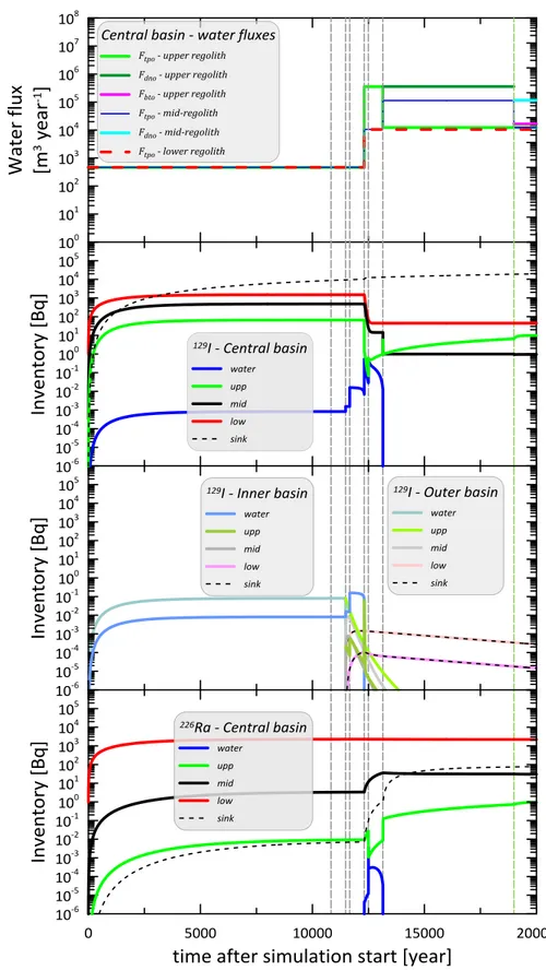
5.2.1. Physical model ... 29

5.2.2. Narrative for radionuclide transport and accumulation... 31

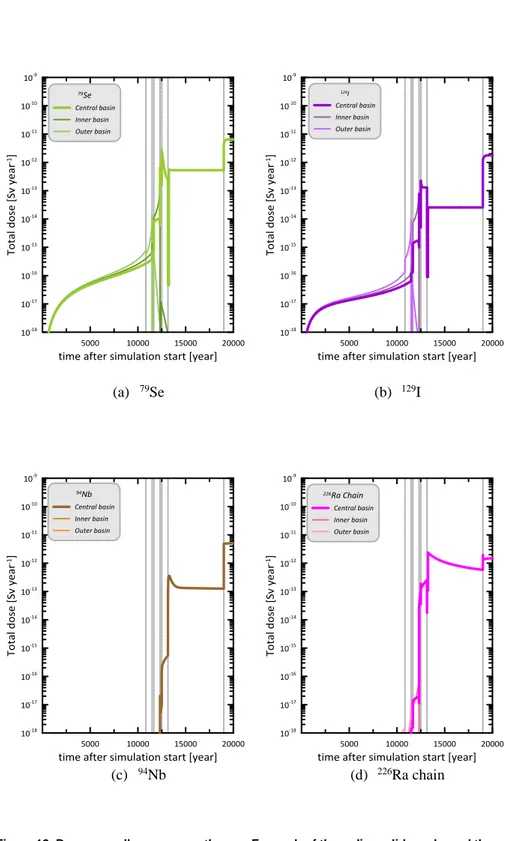
6. Dose assessment and sensitivity study ... 34

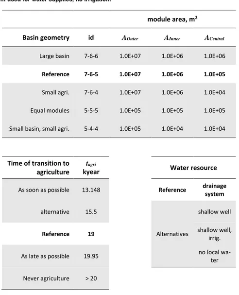
6.1. Overview of calculational cases ... 34

6.2. Reference calculation: 7-6-5, 19 kyear, drainage ... 36

6.3. Time of transition to agriculture ... 41

6.4. Basin geometry ... 43

6.5. Use of water resources ... 45

6.6. Implications for overall uncertainty ... 46

7. Conclusions... 49

8. References ... 50

APPENDIX 1 ... 52

APPENDIX 2 ... 55

1. Introduction

In 2011 the Swedish Nuclear Fuel and Waste Management Company (SKB) submit-ted an assessment of the long-term safety of a KBS-3 geological disposal facility (GDF) for the disposal of spent nuclear fuel and high level radioactive waste in For-smark, Sweden. This assessment, the SR-Site project, supports the licence applica-tion of SKB to build such a final disposal facility.

The biosphere dose assessment carried out as part of SR-Site features a highly de-tailed model of the evolution of the current sea area to the northeast of the planned repository location – the Öregrundsgrepen. Currently submerged, the landscape will emerge over the next few millennia as the land to the southwest has emerged since the end of the previous glaciation. The developing landscape can be assumed to evolve in much the same way. In this way the important transport and accumulation characteristics of the landscape and the patterns of human behaviour leading to po-tential future exposure to any radionuclides released from the disposal facility into the surface hydrological system can be modelled, employing a detailed site charac-terisation programme such as that carried out by SKB over the past decade.

The model employed in SKB’s dose assessment calculations is described by Avila et

al. (2010). This has been reviewed by Kłos et al. (2012) and in greater detail

focus-sing inter alia on the interpretation of hydrology in the model and on the develop-ment of an alternative conceptual model for radionuclide transport and accumulation (Kłos et al., 2014). This report provides details of the development and initial appli-cation of the alternative model, known as GEMA-Site, reflecting SSM’s comple-mentary modelling project over the last decade (see Kłos, 2008). GEMA-Site and the use of simple Reference Biosphere-type models (Walke, 2014) have been used by SSM to investigate uncertainties associated with the modelling of the future For-smark landscape in the context of long timescale radiological assessment.

The model described here gives the basic specification for the GEMA-Site concep-tual model, using a simple approximation to the near-surface hydrology in a single basin in the landscape. The characterisation of the basin employs data taken from Avila et al. (2010) and Nordén et al. (2010). The Kłos et al. (2014) review of hy-drology of objects in the SR-Site assessment is also used together with the interpre-tation of hydrology sketched by Kłos & Wörman (2013a).

Chapter 2 of this report sets out the requirements for the GEMA-Site model. Chap-ters 3 and 4 describe, respectively, the features of the future landscape and concep-tual description of GEMA-Site. Results for a simple interpretation of the evolving system are given in Chapter 5 and an analysis of model sensitivity is given in Chap-ter 6. Project conclusions are found in ChapChap-ter 7.

2. Requirements

2.1. SSM’s independent modelling capability

The Swedish Radiation Safety Authority (SSM) reviews the Swedish Nuclear Fuel Company’s (SKB) applications under the Act on Nuclear Activities (SFS 1984:3) for the construction and operation of a repository for spent nuclear fuel. Since 2004 an independent modelling capability has been progressively developed in order to provide numerical reviews of dose assessment results. The modelling framework is known as GEMA – the generic ecosystem modelling approach and this has been used to review several assessments during this time (Kłos, 2008; Xu et al., 2008). SKB has conducted a detailed site investigation programme that has been used to characterise the site and the surface environment (SKB, 2008). The biosphere com-ponent of this formed the basis for the dose assessment modelling reported by Avila

et al. (2010). The interpretation of the site-descriptive material in SR-Site has been

reviewed by Kłos et al. (2014) and the database for SR-Site (including Nordén et al. 2010) has been used to construct the model “GEMA-Site”, developed to enable a numerical review of the modelling assumptions in the Avila et al. model.

SKB’s biosphere modelling for SR-Site has similarly been developed over the past decade to incorporate increasing site specific detail. As a result the modelling ap-proach differs from the relatively simple and robust formulation of the “reference bi-ospheres” modelling approach. The particular features, events and processes influ-encing the future of the Forsmark site are set out below.

2.2. Site specificity

The degree of site specificity included in an assessment model clearly depends on the site descriptive database. SKB (2008) provides details of the likely evolution (based on the historical record and successionary evidence from the landscape to the southwest). Details from the SKB (2008) database as well as the SR-Site database (Avila et al., 2010; Nordén et al., 2010) have been made available to SSM for use in modelling. Figure 1 illustrates the approximate landscape of the land emerged from the Öregrundsgrepen over the next 5 kyear.

This is the background to the modelling carried out in SR-Site. The landscape covers an area in excess of 150 km2_{. Within the landscape the geology of soils and}

sedi-ments, ecosystems and hydrogeology are combined to describe the drivers of radio-nuclide flow, transport and accumulation in the Quaternary Deposits (QD). Detailed hydrological modelling has been carried out in SR-Site (Bosson et al., 2010) from which the model descriptions of basins in the landscape can be described.

This level of detail is somewhat removed from the traditional methods of biosphere modelling featuring exposure groups based on subsistence farming typically around a well. (See Walke, 2014 for a discussion of how the results from the application of simpler models compare to those obtained in SR-Site by Avila et al., 2010.) Of in-terest is the question: Are there FEPs and combinations of FEPs in the real

land-scape that can combine to produce higher activity concentrations in the accessible environment that are not represented in traditional models or in SKB’s landscape model?

addressed by the simpler methods. In particular the possibility of accumulations dur Figure 1. Landscape at 7010 CE, based on SKB’s topographic map

meufmhoj3085\w001001.adf. Mapped using Global Mapper 12 (www.globalmapper.com). Sea level 30 m below that of the status at 2010 CE. Approximate location of the disposal facility is indicated by the projection of the deposition holes at the surface. Land above sea level at 2010 CE is shown in green and cyan denotes emergent land areas as a result of land rise (at 6 mm year-1_{). Two basins are shown to the northeast of the 2010 CE}

coast-line. Beyond, to the northeast, a sequence of deep lakes are shown as the remnant of the Baltic Sea than once covered the area. Data taken from the Forsmark site descriptive modelling described by SKB (2008). The grid shows areas of 1 km2_.

Figure 2. Shoreline displacement from 10 kyear BP to 10 kyear AP. Data interpreted from Figure 3-3 of Lindborg (2010). The fitted line to the displacement between -6 and +6 kyear is shown. The gradient is close to 6 mm year-1_{. This forms the basis for the evolving}

Using a relatively traditional modelling approach Kłos et al. (2011) and Kłos and Wörman (2013b) have shown that the accumulation in natural ecosystems followed by exposure in agricultural ecosystems can lead to higher consequences depending on the time allowed for accumulation before conversion to agriculture. Attention then focuses on the FEPs leading to accumulation and the timing of the change to agriculture.

Aside from the larger spatial scale of the modelling carried out in SR-Site, compared to traditional reference biosphere models, the main feature is the rapid evolution of the site. Not only is land rise an essential feature of the system than needs to be ac-counted since new land is emerging from the Baltic; the influence that the change in sea level has on the hydrology of the basins and catchments in the landscape is also essential. The following two sections deal with these issues in turn.

2.3. System change

Climate change is the driver of the evolution of the Scandinavian Peninsula (SKB, 2010). At the peak of the latest glacial maximum ice cover at the site is estimated to have been almost 3 km and the crustal depression caused by this loading resulted in the region being submerged by the Baltic following deglaciation. With the load re-moved the land has been rising, as shown in the plot of shoreline displacement as a function of time in Figure 2. These data are interpreted from Lindborg (2010) to il-lustrate the legacy of ice-loading and its removal caused by global warming at the end of the previous glacial episode around 10 – 15 kyear BP. Land rise from -6 to +

6 kyear can be approximated by a rate of around 6 mm year-1 _{as used by Avila et al.}

(2010) in the SR-Site dose assessment modelling.

As indicated in Figure 1 the topography of the Öregrundsgrepen bed and hence fu-ture landscape is relatively flat. It is similar to that inland to the southwest of the Forsmark site. SKB therefore use the basins in the current terrestrial landscape as templates for those anticipated in the emerging landscape. Travelling inland, south-west, from the coast therefore provides a successionary journey from nascent terres-trial ecosystems to fully developed lake, wetland and forest ecosystems. As well as this natural landscape there are towns and habitations with areas of agricultural eco-systems mixed in with natural ecoeco-systems.

In order to model the full evolutionary history of areas of the Forsmark region there is therefore a requirement that the model incorporate system change from fully sub-merged to coastal bay, isolated lake, wetland and forest ecosystems. At any time during the terrestrial period the natural evolution of the site may be perturbed by hu-man actions, most importantly for dose assessments the conversion of suitable land areas to agriculture. Traditionally this has been on the relatively flat and fertile lake bed areas at the centre of the hydrologic basins (Jansson et al., 2006). Extensive ditching is required to convert the natural state – wetland ecosystems – into soils suitable for agriculture. There are therefore numerous changes in thickness, compo-sition, geochemistry and water content that must be accounted in the model of the evolving system. Whereas many of these parameters can be derived from observa-tions (Nordén et al., 2010; Lindborg, 2010) it is the changes to the hydrology of the basins that can be expected to have the greatest influence on the fate of radionu-clides released from fractures in the bedrock.

2.4. Hydrology

Radionuclides enter the surface system of the biosphere primarily in solution in groundwaters than have been in contact with releases from the surroundings of the disposal facility. Water fluxes are therefore the primary driver of radionuclide transport and accumulation.

The bedrock is fractured and these form natural conduits that allow groundwater flows – under this influence of the regional pressure distribution – to reach the top of the bedrock. In general the volumetric flow of contaminated groundwater discharged to the Quaternary Deposits is expected to be low compared to the total circulation in the regolith. Because of the degraded structural integrity of the bedrock surrounding the fractures these locations are more susceptible to erosion and are therefore com-monly found at lower elevations in the landscape. Higher elevations therefore form catchment boundaries, as illustrated by the yellow lines on the map in Figure 1. Kłos & Wörman (2013a) sketched water fluxes in the QD for a typical basin (see Figure 3). Most of the circulation in the QD is derived from the net precipitation to the catchment area. This circulates mainly at higher elevations with gradually reduc-ing flows at deeper levels. Discharge from the bedrock is usually at the lower parts of the basin. Although the fluxes direct from the bedrock are small in comparison to the total water flows in the basin, the circulation illustrated in the sketch focuses the captured net infiltration towards the centre of the basin where it can enhance the up-ward flux entering at the base of the QD, thereby boosting the upup-ward migration of any contaminants entering the regolith from below.

The approach used for dose assessment in SR-Site takes the detailed modelling of the hydrology of six lakes in the present-day terrestrial landscape and from these de-rives an average circulation pattern which is then used as a template for all future Figure 3: Schematic of groundwater discharge from large depths to surface water sys-tems. Because the surface water system is generally located in local topographic minima the relative symmetry in the groundwater flow implies that local flow cells discharge from each side into the near-shore bottoms of the surface water, whereas deeper and more large-scale groundwater flows discharge more or less vertically into central parts of the bottom following a converging stream tube. (Taken from Kłos & Wörman 2013a).

Hill with

high head

Lake /

wetland

Advective

transport

Dispersion

objects (see Chapter 2 of Kłos et al., 2014, reviewing Avila et al., 2010). The GEMA-Site approach is to work with the understanding of the hydrological condi-tions in a “typical basin” and to use this conceptual model to derive fluxes in the ba-sin.

This document describes the initial modelling using an interpretation of the flux map described by Avila et al. Following the Kłos et al. review, requests for further infor-mation were forwarded to SKB with the aim of accessing the details of the water fluxes in the models of the six lakes at different times during their evolution.

2.5. Flexibility: modularisation

The situation is complicated in that the sketch in Figure 3 is a snapshot of the hy-drology at a single time in the evolution of the landscape. The evolving model needs to account for the changes in the flux vectors as the basin transitions from sea bed to bay, to lake to wetland and finally agricultural land.

The approach taken in GEMA-Site is to use compartmental modelling techniques, identifying spatial domains in which the approximation of rapid equilibration of contaminant concentrations is valid. Transfers between the domains are then repre-sented by first order linear kinetics. These issues concern the spatial resolution verti-cally and horizontally in the basin. Also of concern is the change of state of the com-partments in time.

In order to provide a model of the system that is similar to that used in SR-Site the vertical resolution of the QD and water compartments is maintained, namely that of

Lower regolith, Mid-regolith and Upper regolith. When standing water is present a Water compartment is included. Features in the landscape of the basin are therefore

comprised of a set of nested modules as illustrated in Figure 4. The basic module comprises a stack of Low, Mid, Up and Wat compartments. Interactions between compartments and with other modules in the system are then described in terms of the mass transfers between them, primarily via the water flux and solid material flux matrices, respectively F m3 _year-1 _{and M kg year}-1_{. Other processes – for example}

diffusion – can be added as required. In this initial form only water and solid fluxes are explicitly modelled.

Taking a quasi-Lagrangian approach, the size and other physical chemical and biotic characteristics are described by their numerical values and their rate of change. Transfer rates between compartments i and j are given by





1

1

ij i ij ij ij ij i i i i i i i i

F

k M

l

A

l A

k

l

A





 









 

(1) where i

l m thickness of the compartment,

ij

l m year-1 _{thickness of i transferred to j in unit time}

i

A m2 _{surface area of compartment,}

ij

A m2 year-1 portion of surface are of i transferred to j in unit time

i

i

 - volumetric moisture content,

i

 kg m-3 _{density of solid material in the compartment,}

i

k m3 _kg-1 _{dw solid – liquid distribution coefficient,}

ij

F m3 _year-1 _{elements of the water flux matrix, transfers between}

com-partments i and j, and

ij

M kg dw year-1 _{elements of the solid material flux matrix.}

To account for changes in time of the compartment size there are two additional terms to the inter-compartment transfer, depending on the change in compartment size that can be described as moving from i to j (compartment thicknesses and areas, respectively l m year-1 _{and A m}2 _year-1_{). In principal, each of the quantities}

de-fined in Equation 1 can be dede-fined as an instantaneous value and its rate of change. In practice this formalism can be somewhat mitigated by the use of logical state-ments to control transitions (as in Avila et al., 2010). Some parameters, such as the Figure 4: Modular structures of the radionuclide transport model in GEMA-Site. Each compartment in the model has interactions via up- and downslope faces as well as top and bottom faces. The components of the water and solid flux matrices are shown. These combined transfers (see Equation 1) link the compartments of each module and express fluxes into and out of the combined biosphere module. Application of GEMA-Site takes a number of modules and combines them using the lateral spatial discretisa-tion of the system. Input (i) and output (o) fluxes are defined to each of the top (tp), bot-tom (bt), upstream (up) and downstream (dn) faces of the compartments. For example the water flux out of the top of the compartment of Ftpo, the solid material flux entering

from the upstream face is Mupi, etc. These identifiers are used internally to ensure mass

balance in the model – see Appendix 2.

Low Mid Up Wat

upslope

do

wnsl

ope

cmp

Release from bedrock cmp

compartment thickness are smoothly varying functions (eg water depth as a function of isostatic uplift and sedimentation).

With this framework the characteristics of a complete basin can be integrated into the model. In the following chapter the necessary characteristics of the typical basin are discussed followed by the definition of the conceptual model and its application.

2.6. Exposure pathways

The human population of the region can interact with the potentially contaminated areas in each of the basins in many ways. Doses are evaluated for each ecosystem. To facilitate the comparison with the SR-Site LDFs (Landscape Dose Factors – SKB’s indicator of radiological impact in the biosphere) the exact formulations used in Avila et al.(2010) are used. Consumption is reformulated to avoid the unnecessary reliance on carbon consumption that features in the SKB modelling. The exposure pathways calculated are:

Marine ecosystems (Sea/bay stage)

natural ecosystems

(lake/wetland/forest) agricultural ecosystems

Fish (marine) Fish (freshwater) berries

Crustacea (marine) Crustacea (freshwater) mushrooms

water game

berries external irradiation

mushrooms inhalation

game meat

external irradiation dairy products

inhalation green vegetables

root vegetables cereals

drinking water (surface, well)

The amount of consumption takes into account an autarky factor – the degree to which the area of land can support the required level of consumption. Plant concen-trations are derived from both root uptake and interception of contaminated irriga-tion water. This latter opirriga-tion is not used in these initial calculairriga-tions. Details of the expressions are reproduced in Appendix 1.

As the system evolves, the combination of exposure pathways actively involved changes. Marine pathways are only possible during the sea stage. Freshwater fish and crustacea can supplement local foodstuffs during the lake stage. Natural food-stuffs (those available from natural ecosystems) are those that are found in terrestri-alised natural ecosystems but agricultural production requires a significantly modi-fied landscape. It is also possible, at this stage of the evolution, for the other “natu-ral” foodstuffs, berries, mushrooms and game, to be derived from the agricultural system.

Drinking water for humans and livestock is assumed to be obtained from the lake during this stage. As an agricultural area, the model allows water from the surface drainage system or a regolith (ie, shallow) well. Drinking water from uncontami-nated (external) supplies is also allowed.

3. Example system

3.1. Future of the Öregrundsgrepen

Avila et al. (2010) provide a description of the marine parts of the Öregrundsgrepen, describing it as “a funnel-shaped bay of the Bothnian Sea which is a part of the Bal-tic Sea with its wide end to the north and the narrow end southwards”. SKB have produced a digital elevation model (DEM) for the region and this DEM is used to identify 28 sub-basins in the future landscape, based on the bathymetry of the pre-sent-day Öregrundsgrepen. The basins identified by SKB are illustrated in Figure 5. Avila et al., (2010) also note that:

The small-scale topography of the area gives rise to many small catchments with local, shallow groundwater flow systems in the regolith. In combination with the decreasing hy-draulic conductivity with regolith depth, this causes that a dominant part of the near-sur-face groundwater will move along shallow flow paths. Shallow groundwater flow paths imply strong interactions among evapotranspiration, soil moisture content, groundwater levels and flow. In Forsmark, the groundwater table in the regolith is very shallow; in general the depth to the groundwater table is less than a metre. Thus, the groundwater level in the regolith is highly correlated with the topography of the ground surface. This local flow system in the regolith overlies a larger-scale flow system in the bedrock. Each of the basins can be treated as independent from the others in the hydrological modelling (Bosson et al., 2010). In this way, SKB use a combination of detailed modelling MIKE-SHE of representative lakes in the present-day terrestrial biosphere to derive a snapshot of the hydrological characteristics of what they term an “aver-age object”. They further use MIKE-SHE to determine the locations of potential re-lease locations in the future landscape, (see Lindborg, 2010).

3.2. Key features of a typical basin

The development and implementation of the GEMA-Site model requires a repre-sentative landscape object. The intention is to use a generic Forsmark basin as a first step towards a more detailed model. Avila et al. (2010) describe the basins as “lake-centred catchments. For reference, therefore, Basin 116 is selected. As shown in Fig-ure 5, a well-defined lake is expected to develop over the next few millennia and there are several potential release locations associated with it. Although this is not the object in the SKB landscape model that gives rise to the highest landscape dose factors, it does contain all the features necessary for the GEMA-Site implementa-tion.

Figure 6 illustrates Basin 116 with a cross-section between the catchment bounda-ries. This is the representative basin that will be used in subsequent chapters to illus-trate the development of the GEMA-Site model.

As can be seen from the profile, there is a general trend of decreasing elevation to the northeast with the bed of the future lake clearly identifiable in the centre. The shaded area on the map represents the location of the lake based on the current ba-thymetry. As see level falls different parts of the basin will emerge at different times and the succession of ecosystem will begin.

Figure 5: Sub-basins in the Öregrundsgrepen basin, based on present day bathymetry. (Reproduction of Figure 2-2 of Avila et al., 2010). SKB identify basins by a numeric code. Inset is a map from Lindborg (2010) showing all calculated release points (white dots) in the landscape. The selected object is a lake at the centre of Basin 116 at 5000 CE.

Figure 6: Object 116 in the future Forsmark landscape. Map drawn using Global Mapper 12 with the topographic data set provided by SKB. The depth profile shown runs from NE to SW. The basin boundary is indicated and the area of the future lake/wetland is shaded at the deeper part of the basin. Depths are representative of the situation at 2000 CE.

Approximate repository location Lake at centre of Basin 116 at 5000 CE showing release points

SKB's map of potential release locations to the area depicted in Figure 5 shows that the releases are focused on the centre of the future lake (see chapter 6 of TR-10-05; Lindborg, 2010). This is the deepest part of the basin and corresponds, approxi-mately, to the locations of lineaments in the bedrock (Lindborg, 2010). How this is represented in GEMA-Site is discussed in the next Chapter.

4. Conceptual model for the evolution of

the basin

4.1. System identification and justification

Figure 6 illustrates a typical basin in the Forsmark landscape and Figure 3 is a sketch of how deep groundwater mixes with the infiltration over the catchment. The task in GEMA-Site is to capture the concept in Figure 3 in the context of the basin in Figure 6. Clearly some approximation is required in respect of the spatial structures in the basin as well as how the flux vectors in the Quaternary Deposits change as the landscape evolves.

Because the lake is at the centre of the catchment with release to the lowest part of the terrain, the situation of the basin as terrestrial ecosystems with a lake at the cen-tre is first considered as a snapshot. This interpretation is then generalised to con-sider the state of the basin and hydrology at different snapshots during the evolution. In the basin three areas can be distinguished, using the SKB terminology from Avila et al. (2010):

 The water body area – “the lake” - A_aqu

 The terrestrial area surrounding the lake - A_ter

 Subcatchment area, ie the area outside the lake/wetland system- A_SubCatch.

Avila et al. also assume three distinct layers in the QD, namely lower, mid and up-per regolith. Together with a standing water layer, these can be used to identify the water fluxes in the near surface hydrology. Overall the juxtaposition of components in the model suggests a cylindrical geometry, as shown in Figure 7. The water fluxes illustrated in the figure can readily be linked to the modular fluxes shown in Figure 4. The modularisation also suggests that Figure 4’s basic structure can be used to represent the areas in the basin. For the subcatchment and terrestrial areas three compartments can be used, with no standing water compartment. For the aquatic area the water compartment is active.

4.2. Spatiotemporal discretisation

While Figure 7 illustrates one stage during the evolution of the basin, similar to that used in describing the “average object” in SKBs interpretation of the site (Bosson et

al., 2010) it should be appreciated that it is just a snapshot. In order to represent the

distribution of radionuclides entering the basin as it evolves, a representation of the changing conditions in different parts of the structure is necessary.

Figure 8 illustrates how stages in the evolution affect the spatiotemporal discretisa-tion in reladiscretisa-tion to the topography of the basin. From the transect illustrated in Figure 6, a low spatial resolution profile can be proposed, as shown. In this development of the initial version of GEMA-Site three parts of the basin are identified:

 Outer basin (Outer)

 Inner basin (Inner), and

Figure 7: Interpretation of areas and boundaries for a lake-centred catchment. Arrows in-dicate water fluxes (m3 _year-1_{) required to characterise transport and accumulation. The}

three domains of aquatic, terrestrial and uncontaminated sub-catchment are distin-guished.

Figure 8: Topography and spatial discretisation of the basin in GEMA-Site. At early times there is complete water cover for the basin – this is the sea stage. As land rises the outer basin emerges (bay/lake stage). Further land rise (and sedimentation) causes the water columns to be confined to the inner basin (lake/wetland stage) and subsequently the in-ner basin is a wetland and the lake in the central basin. Ultimately the basin drains through a small water body situated in the centre of the basin. Agriculture is possible at any stage in any module where there is a land surface, though attention here focusses on agriculture in the central basin only..

Water terUp terMid Low aquMid aquUp subCatch Low F geo Low F subCatch terMid F subCatch terUp F Low aquMid F Low terMid F aquMid aquUp F aquUp Water F Water terUp F terMid aquMid F terUp aquUp F terUp Water F Water Downstream F terUp Downstream F terMid Downstream F terMid terUp F aquUp aquMid F Water aquUp F terUp terMid F Low Downstream F aquUp terUp F aquMid terMid F terMid Low F aquMid Low F

Aquatic area:

Terrestrial

area:

Subcatchment

area:

Outer basin Inner basin Central basin Sea Lake / bay Lake / wetland Lake / wetland Release from bedrock

Clearly a higher lateral resolution is possible and may be required, depending on the assessment context. For this stage of development, however, three discrete areas suf-fice to illustrate the principle. The modularisation of the model described in Section 2.5 is designed to allow the practical inclusion of additional spatial discretisation. A coarse representation would have a single object (the whole basin). At a higher spa-tial resolution, two modules can represent the outer and inner parts (similar to SKB’s subcatchment + object); with three modules the outer, inner and central basin are distinguished (subcatchment + terrestrial and aquatic objects) and so on.

Figure 8 also shows the local “sea level” at different stages in the evolution. This in-terpretation can be used to identify different temporal domains in the model. Initially the whole basin is covered by sea and this lasts until the end of the “sea stage” at time t_sea [year]. After this stage the landscape forms a bay which gradually contracts to form an isolated lake. This transition occurs at timet_aqu. After this the area is in a

natural state (ie, uninfluenced by human action) and natural ecosystems continue to develop. The time taken for terrestrial species to colonise the emergent land area is denoted by

colony

t . Human action can radically alter the conditions within the

mod-ules. For this reason one more timing event is included: t_agri is the time at which

ag-ricultural ecosystems are imposed within the object by human activity. In practice, transitions in each of the modules identified in Figure 8 can be con-trolled in the model using these parameters. Avila et al. (2010) employ a similar set of "threshold" times to govern changes in the SKB implementation.

Transfers of radionuclides between the spatial domains of each of the modules are described by Equation (1) on page 7. The subscript i denotes the position of the compartment in the network representing the spatial discretisation of the basin. These take the values

 Wat – surface water compartment

 Up – upper regolith

 Mid – mid-regolith

 Low – lower regolith

Each of the parameters in Equation (1) can then be linked to data values representa-tive of the site (cf. Nordén et al., 2010 as interpreted by Avila et al., 2010). In this formalism it is also useful to denote the module associated with each of the parame-ters. In this wayt_sea t_seaOuter,t_seaInner,t_seaCentral_, and so on for all necessary modules in the spatial discretisation.

Equation (1) includes only two spatial translations, namely the water and solid mate-rial flux vectors F and M, the components of which are shown in Figure 4 in relation to each of the faces of the nominal Cartesian compartments structure, namely the in-puts and outin-puts across the faces:

 upstream – upi, upo

 downstream - dni, dno

 top – tpi, tpo; and

Mass balance in the model can therefore be ensured by matching the outputs from one compartment to the inputs to the adjacent. The example of the model imple-mented here is listed in Appendix 2.

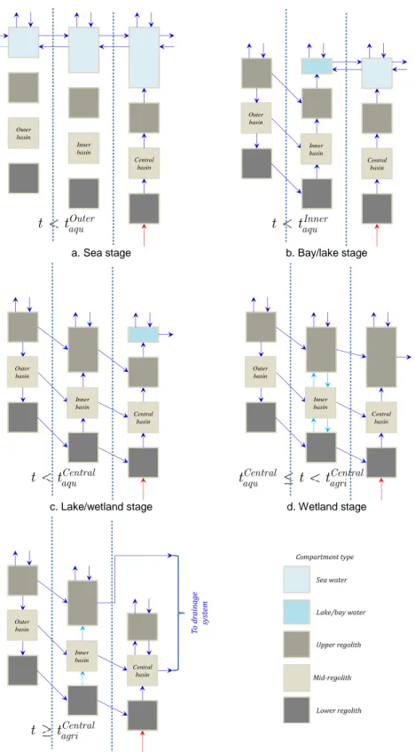
4.3. Fate of radionuclides in the basin: a narrative

The fate of radionuclides entering the basin can be explained by developing the in-terpretation of hydrology shown in Figure 3. Figure 9 illustrates five stages in the development of the three-module model described previously. Release to the basin is from the bedrock fracture at the deepest part of the regolith in the basin (red arrow). There is a small advective pressure from the fracture driving contaminated ground-water from the bedrock into the sediments above the crystalline bedrock.

During the sea stage of the basin’s development (  Outer

aqu

t t ) this small flux, entering

the lower regolith of the central basin, is assumed to continue up through the sedi-mentary material on top of the bedrock, ultimately discharging to the water column of the Central basin. Most of the advective fluxes in the basin are determined by bulk water movements in the Öregrundsgrepen, moving the contents of the water compartments laterally. This is modelled by Avila et al. in terms of the residence time of packets of water in the water column. This approach is also adopted here. There is a relatively small exchange of water with the atmosphere via precipitation and evaporation.

In reality it may be anticipated that the discharge of water from the bedrock, enter-ing the lower regolith, may not reach the water column and that there is considerable dispersion within the intervening regolith layers. Mixing within the lower regolith and other layers is, of course, part of the way in which the spatial domain of the compartment is defined. Diffusive processes within the regolith compartments can also be expected to disperse radionuclides laterally. In this initial version of GEMA-Site, however, diffusive processes are not represented although they are in the Avila

et al. model.

Consequently only the advective flux is represented in the model, causing an upward transport of contaminants from the fracture in the bedrock. Activity entering the base of the lower regolith is therefore transported upwards through the mid- and up-per regolith, entering the water column where it is rapidly disup-persed into the wider sea. Sorption onto solid material in the water column can lead to the transfer of ac-tivity to the upper regolith of the inner and outer basins (and thence deeper into the regolith should bioturbation and diffusion be active). The net result of release dur-ing the sea stage is therefore to accumulate activity in the lower regolith of the cen-tral basin, the mid and upper regolith layers of the cencen-tral basin and the water col-umn. Low concentrations in the water columns in each of the modules disperses small fractions of the total inventory to the regolith in the whole basin.

By the bay/lake stage (  Inner

aqu

t t ) there is a small residual inventory in the upper

regolith of the outer basin, from where the water column has disappeared as a result of land rise. In the outer basin there is a net infiltration through the upper regolith. Some of the infiltration moves vertically to the mid-regolith, some moves to the ad-jacent upper regolith of the inner basin. A similar pattern is assumed in the mid-reg-olith, with transfers to the lower regolith and the mid-regolith of the inner basin. In the lower regolith the transfer is assumed to be constrained to the inner basin’s lower regolith. This is a no-flow boundary condition at the lower surface.

a. Sea stage b. Bay/lake stage

c. Lake/wetland stage d. Wetland stage

e. Agriculture stage

Figure 9: Evolution of hydrology during land uplift. Outer, inner and central basins are shown from left to right. With uplift and sedimentation the water level drops in each mod-ule. Release is to the lowest part of the basin with a small upward flux at all times. As wa-ter levels fall, flow from the ouwa-ter, then inner basin is directed sub-horizontally towards the central basin contributing to increased upward fluxes. Change to agricultural condi-tions necessitates a modified and maintained drainage system.

Outer basin Inner basin Central basin Outer aqu

t

t

Outer basin Inner aqu

t

t

Inner basin Central basin Central aqu

t

t

Outer basin Inner basin Central basin Central Central aqu agri

t

t

t

Outer basin Inner basin Central basin To dr aina ge syst em Central agri

t

t

Outer basin Inner basin Central basin Sea water Lake/bay water Upper regolith Mid-regolith Lower regolith Compartment type

In the inner basin there is now the possibility of an upward flux through the regolith layers to the water column of the bay/lake. This is driven by the flux from the outer basin. As with the distribution of the water fluxes in the outer basin, there is the po-tential for flow from the regolith layers in the inner basin to those in the central ba-sin. The focussing towards the central basin of net infiltration captured in the outer basin contributes to enhanced upward fluxes through the regolith of the inner and central basins. There is exchange of water in the water columns of the inner and cen-tral basins and there is a loss from the water of the cencen-tral basin that is still in direct contact with the remaining Öregrundsgrepen. During this period the thickness of the upper regolith in the inner basin also increases as a result of sedimentation.

By the lake/wetland stage ( _ Central

aqu

t t ), the lake provides the downstream outlet for

the basin. This is in the central basin and there is surrounding wetland that has accu-mulated upper regolith material during the lake/bay phase of the inner basin. The outer basin – at higher elevations – is likely to consist of forest ecosystems that have colonised the emergent land surface, with a thin layer of upper regolith compared to the inner and central basins where there are greater accumulations of sediment. At this stage of development the intercepted net precipitation in the outer basin is again directed downwards and inwards towards the lower parts of the basin. Poten-tially there is still a small upward flux in the inner basin. As before there is an in-creased flux entering the domain of the central basin, allowing for the inin-creased overall water flux due to the captured infiltration. A precise map of the distribution of the fluxes requires sophisticated modelling (cf. Bosson et al., 2010) but there will be increased upward flux from the lower to mid- to upper regolith in the central ba-sin, acting to drive any accumulation of radionuclides at the interface between the bedrock and the regolith upwards. During this phase there is ongoing accumulation in the upper regolith of the central basin and the depth of the water column in the central basin is decreasing due to uplift and sedimentation.

Radionuclides may continue to enter at the base of the central basin and move up-wards due to the bedrock-to-lower regolith flux. The upward flux at the top of the lower regolith is increased due to the contribution of the captured infiltration enter-ing from the sides of the lower regolith in the inner basin. In addition to the radionu-clide flux from the bedrock, any (albeit small) accumulations in the compartments of the outer and inner basins will circulate with the water fluxes around the compart-ments of the modules in the basin.

In this three module representation of the basin, the final stage of natural evolution is the pure wetland stage ( Central   Central

aqu agri

t t t ). The water table remains close to the

surface, especially in the inner and central basins. As interpreted here this means that what loss there is from the basin is from drainage of the upper regolith in the central basin. There may be semi-permanent streams during this period. A more complete model of the basin would include these explicitly. Again, the most im-portant issue for the model is the representation of flux vectors between the regolith layers of the outer, inner and central basins. The loss from the central basin must take into account all inputs (across the geosphere-biosphere interface plus inter-cepted infiltration from outer, inner and central modules).

Overall, the fate of radionuclides entering the basin is to circulate from the lower regolith of the entry point. If there is little retention (weakly sorbing species) there will be significant loss from the system. Nevertheless there will be recirculation around the basin. More strongly sorbed radionuclides will be retained at deeper lev-els. The increased flux in the lower regolith of the central basin occasioned by the

capture of relatively large volumes of infiltration in the inner and outer basins will act to accumulate activity in the upper regolith of the central basin. Kłos and Wör-man (2013a) and Kłos et al. (2011) have shown the potential importance of high ac-cumulation in natural ecosystem prior to conversion to agriculture.

The agricultural stage ( _ Central

agri

t t ), has a drainage system imposed on the natural

landscape’s drainage by the human population. As shown only the central basin is assumed to be used for agriculture. In principle though, any of the modules could be

converted at time  module

agri

t t , for module = Outer, Inner, Central. In this case, the

large combined volumetric flow from the outer and inner basins that would enter the upper regolith of the central basin is diverted in excavated ditches so as to bypass the central area. Drains are also emplaced in the mid-regolith of the central basin so as to prevent the net infiltration in the central basin from saturating the agricultural soils. There is residual flow from the mid- and lower regolith layers in the inner and outer basins. NB, this interpretation does not account for irrigation, which is mod-elled, as required, as an abstraction with interception by the crop before flowing to the upper regolith.

The key to the model is therefore understanding water inputs and losses from the ba-sin and understanding the internal variation in time and space of the water flux vec-tors between the different regolith layers. Chapter 5 of this report interprets the basic lake/wetland snapshot (the “average object” from Bosson et al., 2010) as used in the Avila et al. (2010) modelling for SR-Site.

5. Application: region specific basin

5.1. System description

5.1.1. Basin characteristics

The GEMA-Site model focusses on interpretation of the hydrology in the basin. Wa-ter fluxes in the basin are overwhelmingly dictated by the infiltration of captured precipitation. In other words, the hydrology is determined by the size of the catch-ment and the physical characteristics of the material in the basin. The model is im-plemented in Ecolego (Facilia, 2013).

Table 1 lists the numerical values of the region specific characteristics of the model. These include the regional precipitation (P m year-1_{) and evapotranspiration (E m}

year-1_{) as well as the assumed values for the advective velocity of water entering at}

the base of the lower regolith, carrying with it radionuclides in solution. SKB distin-guish release from the bedrock under marine and terrestrial conditions (Bosson et

al., 2010) but there is some question of interpretation (see Section 5.1.3 below). The

release flux during the sea stage is set to v_{geo sea,} v_{geo ter,} = 0.01 m year-1. A constant

land uplift rate is assumed over the period of the modelling, derived from Figure 2. The total volumetric throughput is determined by the areas of the different modules in the basin. Table 2 lists the areas in the Avila et al. model for the objects shown in Figure 5. Taking Object 116 as reference in the definition of the GEMA-Site model is helpful in the sense that the averaged areas are similar. The mean basin size over the whole landscape is 107 _m2 _{with the “lake”}1 _{being 8.5×10}5 _m2_{. Object 116 has a}

basin area of 1.4×107 _m2 _{and a “lake” area of 1.6×10}6 _m2_.

In the GEMA-Site interpretation the three modules are identified as follows:

 Outer basin – taken to be the overall size of the basin (implicitly less the area

of the inner basin). For initial modelling purposes, therefore _A0Outer _{= 10}7 _m2_.

 Inner basin – the maximum lake area (less the area of the central basin). 0Inner

A = 106 m2.

 Central basin – there is no specific information from the SKB database on the

dimension of this part of the basin. The profile in Figure 6 is useful in this re-spect. A value of ₀Central

A = 105 m2 is used for these initial modelling purposes.

Table 3 summarises the characteristics of the three GEMA-Site modules.

1 _{SKB have a fixed size for the lake and wetland combined in their modelling. This}

area is the maximum extent of the lake and wetland. In GEMA-Site, with the three module spatial discretisation, the area with standing water – the lake – changes in size during the evolution. The size of the lake denoted by Lindborg (2010) is there-fore the area of the depression in the basin around which the highest closed contour can be drawn. Above this level there is contact with the sea. This approach is used in Figure 6 to identify the location of the lake in basin 116 in the GEMA-Site defini-tion. This area is identified as the area of the inner basin.

Table 1: Region specific details for the implementation of GEMA-Site described here.

Parameter Value Module Description

P m year-1 _{0.56 all basin Precipitation (Lindborg, 2010)}

E m year-1 _{0.4 all basin} Evapotranspiration (Lindborg

(2010)

, geo sea

v _{m year}-1 _{0.01 all basin}

Bedrock adv. velocity sea stage (Bosson et al., 2010). Central basin only.

, geo ter

v _{m year}-1 _{0.01 all basin}

Bedrock adv. velocity non-sea stage (Bosson et al., 2010). Central basin only.

_wat year-1 _{0.017 All basin} Residence time of water parcels in

grepen (Aquilonius, 2010)

uplift

l

m year-1 _{-0.006 all basin} Isostatic uplift rate, interpreted

from SKB(2010), see Figure 2

Table 2: Catchment areas of objects in the SR-Site landscape model. Data taken from Ta-ble 7-5 of Lindborg (2010), quoting data from Löfgren (2010). Object 121 is modelled as three distinct areas with a lake in only one of them. The date at which the land first emerges from the Baltic and the time at which the sea is finally absent are shown. Object 116 is emphasised.

SR-Site

object basin area m2 _{lake area m}2 _{First land CE Last Sea CE}

101 2.18E+07 3.36E+05 1997 8015 105 3.56E+07 1.36E+06 798 11,156 107 4.84E+06 1.43E+06 669 3497 108 7.58E+06 1.42E+06 767 5011 114 2.63E+07 2.66E+06 -1185 8545 116 1.41E+07 1.60E+06 757 4783 117 1.61E+07 1.87E+06 -1347 2997 118 2.00E+06 3.60E+05 287 2848 120 1.03E+07 3.01E+05 -1725 2409 121_1 3.56E+06 2.38E+05 486 4007 121_2 8.92E+05 876 2865 121_3 6.38E+05 765 3620 123 7.71E+06 4.66E+05 261 6482 124 2.44E+05 8.27E+04 574 1888 125 4.21E+05 7.61E+04 693 1902 126 6.25E+06 5.60E+05 477 4379 136 3.59E+06 6.11E+05 53 1898 146 3.82E+06 2.42E+05 255 4748

mean 1.04E+07 8.51E+05

max 3.56E+07 2.66E+06

Table 3: Numerical values used in the definition of the GEMA-Site modules for a repre-sentative basin. Values are based on a projection of land rise for the map shown in Fig-ure 6 with land rise at 6 mm year-1_{. See text for details.}

Parameter Units Value Scope Comments

0

A _m2 ₁₀5 _{Central Basin Initial object area}

bay

l _{m 5 Central Basin Depth on isolation from sea}

colony

t _{year 100 Central Basin Time for terrestrial colonisation}

agri

t _{year 19000 Central Basin Time of conversion to agriculture}

min

l _{m 0.01 lower regolith Minimum allowed thickness}

0

l _{m 1 lower regolith Initial thickness}

min

l _{m 0.01 mid regolith Minimum allowed thickness}

0

l _{m 0.9 mid regolith Initial thickness}

min

l _{m 0.01 upper regolith Minimum allowed thickness}

0

l _{m 0.1 upper regolith Initial thickness}

,

agri root

l _{m 0.3 upper regolith Agricultural rooting zone}

min

l _{m 0.2 water Depth at end of aquatic state}

0

l m 80 water Initial water depth

0

A _m2 ₁₀6 _{Inner Basin Initial object area}

bay

l _{m 5 Inner Basin Depth on isolation from sea}

colony

t _{year 100 Inner Basin Time for terrestrial colonisation}

agri

t _{year 25000 Inner Basin Time of conversion to agriculture}

min

l _{m 0.01 lower regolith Minimum allowed thickness}

0

l _{m 1 lower regolith Initial thickness}

min

l _{m 0.01 mid regolith Minimum allowed thickness}

0

l _{m 0.9 mid regolith Initial thickness}

min

l _{m 0.01 upper regolith Minimum allowed thickness}

0

l _{m 0.1 upper regolith Initial thickness}

,

agri root

l _{m 0.3 upper regolith Agricultural rooting zone}

min

l m 0.2 water Depth at end of aquatic state

0

l _{m 75 water Initial water depth}

0

A _m2 ₁₀7 _{Outer Basin Initial object area}

bay

l _{m 5 Outer Basin Depth on isolation from sea}

colony

t _{year 100 Central Basin Time for terrestrial colonisation}

agri

t _{year 25000 Outer Basin Time of conversion to agriculture}

min

l _{m 0.01 lower regolith Minimum allowed thickness}

0

l _{m 1 lower regolith Initial thickness}

min

l _{m 0.01 mid regolith Minimum allowed thickness}

0

l _{m 0.9 mid regolith Initial thickness}

min

l _{m 0.01 upper regolith Minimum allowed thickness}

0

l _{m 0.1 upper regolith Initial thickness}

,

agri root

l _{m 0.3 upper regolith Agricultural rooting zone}

min

l _{m 0.2 water Depth at end of aquatic state}

0

Following the example of the SR-Site modelling, GEMA-Site is setup to model the evolution of the basin from the end of the glaciation to several thousand years in the future. Initially then, the Baltic covers the entire site to a depth of several tens of me-tres, as in Figure 2. From Löfgren (2010) the initial depth of the central basin is taken to be 80 m and, as a simplification, each of the modules suggested by the pro-file in Figure 6, the mean elevation of each of the modules is taken to be 5 m higher. Therefore

 _l0Central _{= 80 m}

 _l0Inner _{= 75 m}

 _l0Outer _{= 70 m}

The values therefore represent a mid-sized object with a central part of the basin 10 m deeper than the outer basin.

For each of the modules the initial and minimum thickness of compartment layers are set. The initial thicknesses are taken from the definition of the sea stage in Avila

et al. (2010). The initial state of the regolith thicknesses are therefore the same in

each module – 1m for the lower regolith, 0.9 m for the mid-regolith and 0.1 m for the upper regolith. Organic material accumulates at the surface, increasing the thick-ness of the upper regolith. On conversion to agricultural land this is compacted and the thickness reduced. The thickness of the rooting zone for agricultural ecosystems can be set for each module (although here only the basin is used for farming). A value of 0.3 m is assumed corresponding to the Avila et al. model.

The minimum thicknesses set to avoid numerical problems as the water level de-creases or the media in the regolith layer is eroded. Section 5.1.2 describes the tim-ing of events in the model in more detail.

Other numerical data for the media in the basins are described in Appendix 3 for both nuclide specific and non-specific parameters.

5.1.2. Timing parameters and evolution

At some stage during the rise of the sea bed, the water in the basin becomes isolated from the rest of the bay. The time of conversion is defined in the same way for each

module, namely when the water level drops below l_bay = 5 m.

There are four transitions in the evolution of each module.

 t_sea – transition from sea to bay

 t_aqu – end of the aquatic period (no standing water in the module: water

com-partment disconnected and inventory redistributed)

 t_colony – the time taken for colonisation of the emerged land by terrestrial biota.

A value of one hundred years is assumed

 t_agri – the time at which transition to agricultural conditions is imposed by the

local human population. In Table 3 only the Central basin is converted to agri-cultural land in the modelling interval of 20 kyear, with Central

agri

The sea-bay and end of the aquatic periods are determined at run-time, depending on uplift and sedimentation. for each of the modules, therefore:









0           bay sea

uplift tpi tpo obj gl

bay aqu sea

uplift tpi tpo obj peat

l l t l M M A l t t l M M A (2)

During the sea stage the sediment material is assumed to be equivalent to the glacial clay that constitutes the bed of the Öregrundsgrepen. Density is of the clay is_gl, kg

m-3 _{from Lindborg (2010). The material deposited during the aquatic phase after the}

sea stage is similarly calculated but the density is that of peat (peat, kg m

-3_{) that}

ac-cumulates at the bottom of Swedish lakes. Numerical values are taken from Lind-borg (2010). The net sedimentation considers the balance of solid material fluxes at the top of the upper regolith compartment M_tpiM_tpo, kg year-1.

5.1.3. Water, solid material fluxes and mass balance

Equation (1) shows how transfer rates are evaluated in the model. It places a strong emphasis on the water and solid material fluxes from the ith _{to the j}th _{compartment in}

the network. Practically, this means that each snapshot in Figure 9 requires a sepa-rate flux map for each module. There are then five sets of fluxes to be determined using the parameters in Table 1 and Table 3. For reference, full details from the model are given in Appendix 2. There is some repetition and not all the flux maps differ greatly between snapshots. The following provides an overview of the method as applied to part of the evolution.

During the sea stage the only advective flux in the regolith is that from the geo-sphere, therefore in the Central basin

, , ,

, 0 , , ,

    

 

Central Central Central Central Central Central low bti geo obj low,tpo mid bti mid,tpo upp bti

Central n bto

F v A F F F F

F n low mid upp wat

(3)

ie, this flux propagates upwards through the regolith column of the central basin un-til it enters the water compartment. There is no downward flux in the regolith or from the water compartment but there are lateral exchanges between the water col-umn of the central basin and adjacent modules2_:

2 _{Mass balance is explicitly addressed in this model. The three terms in addition to}

the turnover time are an expression of this but are small in comparison with the overall exchange of volumes of water in the water column. As a consequence of mass balance being explicit, water input from outside the modelled area is included from “upstream” and “downstream” directions in the conceptual model. Transfers out of the system carry radionuclides in solution but inflows do not. Implicitly, therefore, the water volume outside the model has zero concentration.

, , , ,



      _    _   Central Central Central Central Central Central wat

wat upi wat upo wat dni wat dno obj _Central geo wat

l

F F F F A v P E , (4)

As indicated in Figure 9, any activity entering the central basin therefore enters the sea and is distributed throughout the system. Transfer of radionuclides to the rego-lith compartments of the inner and outer basins only arises as a result of sedimenta-tion: , , , , ,      m m

wat bto upp tpi ned

m m

upp tpo wat bti upp

M M s

M M s

m Inner Outer

(5) Table 4: Summary of fluxes in the modules of the modelled basin at the different snap-shots in Figure 9. Implementation is described for selected cases here. For full model im-plementation see Appendix 2.NB, although each part of the basin could be converted to agriculture, this interpretation assumes that only the central basin is converted during the 20 kyear period modelled.

Evolution

snapshot Module Characteristics of the flux map

Sea (Figure 9a)

All Described. Most water exchange in the water column. Explicit representation of bedrock driven transport in central basin regolith.

Bay/Lake (Figure 9b)

Outer Described. Fluxes driven by net precipitation. Flux vectors in-terpreted as vertical and lateral components

Inner Described. As Sea stage with additional input from Outer basin Central As sea stage. Lake/ Wetland (Figure 9c)

Outer As bay/lake stage

Inner Similar to outer basin bay/lake stage but with additional up-stream inflows

Central Similar to Inner basin bay/lake, simplified lake water drainage Wetland

(Figure 9d)

Outer As bay/lake

Inner As lake/wetland

Central Similar to inner basin, lake/wetland stage. Drainage from up-per regolith compartment

Agriculture (Figure 9e)

Outer As bay/lake

Inner As lake/wetland, upper loss to drainage not central compart-ment. Does not affect mass balance in inner basin

Central Modified, basin drainage from central mid and exchange be-tween up-per and mid compartments