00:30 Essential Parameters in Eddy Current Inspection

(1)

SKI Report 00:30

ISSN 1104-1374 ISRN SKI-R--00/30--SE

Essential Parameters in Eddy

Current Inspection

Tadeusz Stepinski

(2)

SKI Report 00:30

Essential Parameters in Eddy

Current Inspection

Tadeusz Stepinski

Signals and Systems

Uppsala University

P O Box 528

SE-751 20 Uppsala

Sweden

May 2000

This report concerns a study which has been conducted for the Swedish Nuclear Power Inspectorate (SKI). The conclusions and viewpoints presented in the report

(3)

Summary

This study has been conducted for and supported by the Swedish Nuclear Power Inspectorate (SKI).

Our aim was to qualitatively analyze a number of variables that may affect the result of eddy current (EC) inspection but because of various reasons are not considered as essential in common practice. In the report we concentrate on such variables that can vary during or between inspections but their influence is not determined during routine calibrations. We present a qualitative analysis of the influence of the above-mentioned variables on the ability to detect and size flaws using mechanized eddy current testing (ET).

ET employs some type of coil or probe, sensing magnetic flux generated by eddy currents induced in the tested specimen. An amplitude-phase modulated signal (with test frequency f0 ) from the probe is sensed by the EC instrument. The amplitude-phase modulated signal is amplified and demodulated in phase-sensitive detectors removing carrier frequency f0 from the signal. The detectors produce an in-phase and a quadrature component of the signal defining it as a point in the impedance plane. Modern instruments are provided with a screen presenting the demodulated and filtered signal in complex plane. We focus on such issues, related to the EC equipment as, probe matching, distortion introduced by phase discriminators and signal filters, and the influence of probe resolution and lift-off on sizing. The influence of different variables is investigated by means of physical reasoning employing theoretical models and demonstrated using simulated and real EC signals. In conclusion, we discuss the way in which the investigated variables may affect the result of ET.

We also present a number of practical recommendations for the users of ET and indicate the areas that are to be further analyzed.

(4)

Sammanfattning

Denna rapport är utförd för och finansierad av Statens Kärnkraftinspektion. Arbetet utfördes vid Avd. för Signaler och system, Uppsala universitet.

Syftet var att kartlägga och kvalitativt analysera ett antal faktorer som påverkar provningsresultatet vid virvelströmsprovning och bör därför kvalificeras som viktiga variabler vilka påverkar provningsresultat.

I rapporten beaktas speciellt sådana variabler som kan variera under eller mellan provningar, men deras inverkan fastställs inte vanligtvis vid de normala kalibreringar eller kalibreringskontroller som tillämpas. En kvalitativ analys av inverkan av dessa detekterings- och storleksbestämnings förmågan vid mekaniserad virvelströmsprovning presenteras.

En virvelströmsprovning fodrar en prob och ett virvelströminstrument som detekterar små förändringar i probens impedans eller i dess utgångsspänning. Instrumentet består av en ingångskrets, demodulator och skärm. Den amplitud-fasmodellerade signalen från proben förstärks och demoduleras i instrumentet för att presentera den som en punkt i ett komplext plan. Egenskaper hos instrumentets alla beståndsdelar påverkar provningsresultatet. I rapporten analyseras separat interaktion sökare – instrument, olika typer av fasdiskriminatorer och deras prestanda, samt signalfilter som används för att minska lift-off inverkan. Separat betraktas probens upplösnings- och lift-off - effekter på storleksbestämningen. Som resultat av analysen definieras ett antal viktiga variabler och deras inverkan uppskattas med hjälp av fysikalisk argumentation genomförd med hjälp av teoretiska modeller och illustrerad med resultat av digitala simuleringar.

I slutsatser ges praktiska rekommendationer samt förslag på områden vilka kräver ytterligare studier.

(5)

1. Introduction

Different parameters affect the outcome of non-destructive test (NDT) in different ways, those parameters that determine the result of an inspection are defined as essential

parameters (EP).

Essential parameters related to any particular inspection can be associated to different parts of the inspection and divided into three groups: input parameters, procedure parameters and equipment parameters. ENIQ in its Recommended Practice (ENIQ, 1998) splits those groups into parameter sets that can be influential in inspection of steam generator tubes with eddy current technique (ET).

Table 1. Classification of the parameters essential for ET.

Input Group Procedure Group Equipment Group

Environmental parameters Probes EC system parameters

Defect parameters Scanners Probe parameters

Method and personnel Scanner performance

Essential parameters have received considerable attention recently, especially in the nuclear field, due to the growing demands on the reliability, repeatability and accuracy of non-destructive testing. NDT that has been an independent field for many years starts using, such tools as, measurement error, probability of detection (POD), or receiver operating characteristic (ROC), the tools that have been already established in measuring engineering and communications for a long time. In this situation it becomes important defining eddy current (EC) instrument and specify its essential parameters in a way similar to that used for any other measurement instrument or communication receiver.

In this preliminary study we will focus on such issues related to the EC equipment and the employed procedure as, probe matching, performance of phase discriminators, EC pattern parameters in the impedance plane, as well as the influence of lift-off, probe resolution and scanning speed on defect sizing.

The goal of this study is qualitative analysis of the influence of the above mentioned factors on the ability to detect and size flaws using mechanized ET. The influence of different variables will be investigated by means of physical reasoning employing theoretical models, and demonstrated using simulated and real EC signals. The study will not include simulations of electromagnetic fields related to various defect parameters and coil configurations. The study should result in a number of practical recommendations for the users of ET and should indicate the areas that are to be further analyzed.

(7)

1.1. Eddy current instrument

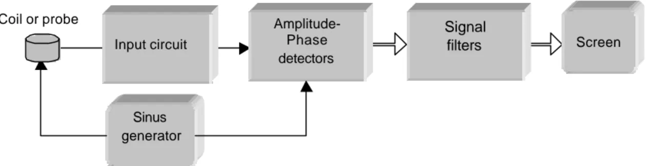
Eddy current inspection employs some type of coil or probe sensing magnetic flux generated by eddy currents induced in the tested specimen. The simplest way of inducing and sensing eddy currents in the inspected material is using a coil shaped respective to the application. A sine generator feeds the coil with constant current with some test frequency and the coil impedance is sensed by the instrument.

An EC probe consists of at least two windings, a primary winding used for inducing eddy currents in a specimen, and a secondary winding (pick-up) sensing flux changes resulting from the variations in density of eddy currents. Probes deliver modulated sine voltage at the output of the pick-up coils. Modern EC instruments (see block diagram in Fig. 1) can accept both coils and probes at the input. Coils require the use of impedance bridge circuits at the instrument input. The input impedance bridge converts coil impedance to a sine voltage and also performs coil balancing. Generally, probes do not require impedance bridges at the input but they also need means for balancing.

Figure 1. Block diagram of an EC instrument

The amplitude-phase modulated signal from the input circuit is amplified and demodulated in phase sensitive detectors removing carrier frequency from the signal. The detectors produce an in-phase and a quadrature component of the signal defining it as a point at the impedance plane. Most modern instruments are provided with screen presenting the demodulated signal in complex plane.

2. Input circuits – probe matching

For correct matching of the probe to a particular EC instrument it is essential to know what type of input circuit is used in the instrument. An impedance bridge requires some more care than simple asymmetrical inputs used in many modern instruments. Below we will consider characteristics of both types of input circuits separately.

2.1. Impedance bridge

An impedance bridge is the simplest possible EC instrument and a classical input circuit of electronic EC instruments. Indeed, an impedance bridge and a cathode tube display were used as the first EC instruments (ASNT NDT Handbook, 1996).

Impedance bridge has two functions, it converts coil impedance to an amplitude-phase modulated sine voltage and performs coil balancing. The first function is required for simple coils that are used rather seldom today (mostly in applications with space

Screen Input circuit Amplitude-Phase detectors Coil or probe Signal filters Sinus generator

(8)

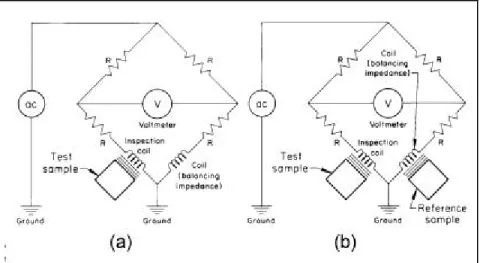
limitations). However, this circuit is also very useful for probes, especially those employing differential pick-ups. The importance of the impedance bridge results from its second function, probe balancing. Balancing operation is required for any type of probes and coils, both absolute and differential. During balancing coil impedance is compensated which results in shifting working point from the impedance diagram to the origin of coordinates. This operation for coils is performed using either a balancing coil or a reference coil (see Figure 2). Balancing of a probe with differential pick-ups can be performed using bridge shown in Figure 3. Balancing of absolute probes and coils compensates the signal on the surface of defect-free specimen, while balancing of differential probes compensates probe unsymmetry. Generally, balancing makes possible amplification of the modulated signal to enable sensing its small variations in response to the detected flaws. Balancing is a very essential function of the EC instrument since it affects its linearity and dynamic range.

Figure 2. Impedance bridges for simple coils. (a) With balancing impedance (b) With

reference sample (reprinted with permission from ASM Handbook, 1996).

Impedance matching in case of simple absolute coils (Figure 2) is essential for the inspection and directly influences test performance. Here, even cable impedance and its temperature variations are essential for the test. Care should be taken to avoid the risk of probe resonance by choosing sufficiently low frequency.

a b

Figure 3. Typical impedance bridges of EC instrument. (a) For direct differential coils.

(9)

For the differential probes and coils impedance matching (Figure 3) has smaller influence on the test result but some care should be taken to ensure matching between the bridge resistors and coil impedances. Large impedance mismatch may result in balancing problems and may decrease the signal to noise ratio (SNR).

2.2. Asymmetric input

Many modern instruments have a simple asymmetric input suitable for internally balanced differential probes. Using other probe types with such instruments requires adapters containing external bridges.

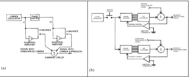
An internally balanced probe has a number of windings connected in this way that their output should be very small (theoretically zero) if the probe is placed in the air or on a surface of a defect free specimen. It should be noted however that it is very difficult to manufacture perfectly balanced probes and some unbalance signal will always be present. The amount of unbalance signal depends on the test frequency and the inspected material. Impedance matching is not essential in this case since the impedance of the input amplifier is much higher than output impedance of the probe. Cable length should not influence much test results for such instruments, except decreasing the SNR which would be lower for long cables. However, probe balancing requires more sophisticated digital circuits of the type shown in Fig. 4 (ASNT NDT Handbook, 1996). The balancing is performed by adding to the unbalanced signal (unbalanced carrier) sine and cosine components canceling it at least partly. Total cancellation is impossible due to harmonic components always present in the probe output.

(a)

(b)

Figure 4. Typical balancing circuits. (a) Manual with potentiometers. (b) Automatic

with counters (reprinted with permission from ASNT NDT Handbook, 1996).

Since automatic balancing circuits are rather complicated and expensive many manufactures resign of direct balancing and replace it with DC compensation after the phase detectors. This solution should work properly unless the unbalance signal and the amplification are not too high. A high unbalance signal amplified before the demodulation may namely result in saturation of some circuits before or in the detectors. This in turn will cause distortion of the modulated signal and substantial errors at the output of the detectors. It is a very important issue since the user generally does not have access neither to the unbalance signal from the probe nor to the signal at the detector input. In practice the user may not be aware when this problem occurs. This

(10)

means that using such instruments requires very well designed and manufactured probes that do not produce significant unbalance signal. This is even more important when using multiple-frequency systems that excite probes at several frequencies simultaneously.

To conclude discussion on matching probes to the input circuits we can name the following essential parameters:

• Probe unbalance signal for internally balanced probes • Type of balancing circuit in the EC instrument

To avoid problems with probe mismatch we would like to recommend the following: • Use always well designed and balanced probes and coils.

• Be aware of internal design of your instrument and use it in a proper way when preparing new inspection.

• Special care should be taken when using simple coils. Cable length and impedance matching are very important.

• Avoid using instruments without balancing circuits.

• Be aware that using a very high gain may result in high harmonic distortion in the modulated signals.

3. Phase sensitive detectors

Output signal from the input circuit of a modern EC instrument takes the form of amplitude-phase modulated signal which depends on probe position x

where:

A(x), φ(x) – amplitude and phase of the signal

x – probe position on the specimen (we assume scanning in one direction only) f0 – test frequency

In the first EC instruments this signal was fed directly to the Y-electrodes of a cathode ray tube while the reference sine signal was connected to the X-electrodes. Characteristic ellipse curves were obtained in this way and A(x), φ(x) could be red out from the ellipse.

Modern EC instruments employ amplitude-phase detectors that suppress the carrier frequency and produce a vector (point) in the screen defined by amplitude A(x) and phase φ(x). However, not many users are aware that different circuits can be used for this purpose and although all of them should operate properly in nominal conditions, they behave differently if the signal VSIG(t,x) is not a perfect sine wave. Below, we will present a short description and an analysis of three main detector types and compare their performance using numerical simulations.

0 0 0 ( )]; 2 sin[ ) ( ) , (t x A x t x f VSIG = ω +φ ω = π

(11)

3.1. Multiplying detector

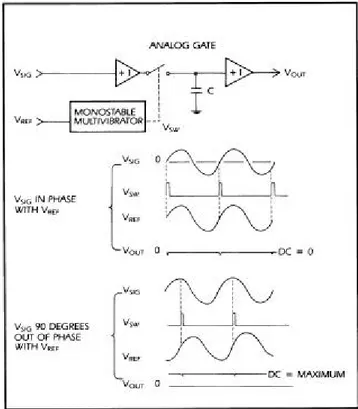
Theoretically, amplitude demodulation should be performed by multiplying the input signal VSIG(t,x) by the reference signals sin(ωt) and cos(ωt) followed by low-pass filtering suppressing the second harmonic of the carrier frequency. This operation is normally performed on an analog signal and requires analog multipliers. Operation principle of such detectors is illustrated in Fig. 5. Input signal VSIG is applied to an analog multiplier together with the reference sine wave VREF. A direct product of both signals takes the form of a sine wave with double frequency and a DC component that is proportional to A(x)cos{φ(x)}.

Figure 5. Operation principle of multiplying

detectors (reprinted with permission from ASNT NDT Handbook, 1996).

If the reference is shifted 90° in phase and multiplied with the signal the DC component of the product will be proportional to

A(x)sin{φ(x)}. This means that

if the double frequency terms are suppressed by low-pass filtering, the DC components will become directly the In-phase and the Quadrature component of the input signal

VSIG. This is theory, in practice

VSIG is never a pure modulated sine, it has some harmonic components that introduce errors at the output. Also, real analog multipliers produce a considerable amount of noise at the output. To analyze these effects we performed numerical simulations of different detector structures and compared the results (cf. Section 3.4).

3.2. Detector with square wave

The demodulation operation can be made in a simpler way. Square wave can be used instead of the VREF to eliminate the multipliers. The square wave must have the same

phase as the reference signal. The multiplication with a square wave can be realized using a simple diode ring shown in Fig. 6. The diode ring operates as a full wave rectifier and switching points of the diodes are controlled by the reference VREF . The

diodes 1 & 3 trade role with diodes 2 & 4 depending on the polarity of the reference voltage.

(12)

Figure 6. Example of detector with diode ring

(reprinted with permission from ASNT NDT Handbook, 1996).

In the example shown in Fig. 6 transformers are used to produce symmetrical signals required by the ring but this can be done using transistors. When the two halves of each transformer are symmetrical with respect to the center taps, no component of the reference voltage or input voltage will be present in the output signal. Using diodes simplifies the detector circuit and enables its proper operation for higher carrier frequencies that can reach several MHz in some EC applications. Such detector is simple and robust. It is not sensitive to noise due to averaging by the low-pass filter that follows the diode ring.

3.3. Sampling detector

A sampling detector operates on a very simple principle, sampling the input signal at time instants depending on the detector phase. It is simple but sensitive to noise which means that it requires a noise free pure sine wave for proper operation.

Figure 7. Operation principle of sampling

detector (reprinted with permission from ASNT

Its operation principle is illustrated in Fig. 7. It consists a sample-and-hold circuit synchronized by the reference signal. The S-H circuit samples the input signal in time instants defined by the reference. If VSIG is a pure sine theoutput of the

S-H can be expressed as

) sin(

)

(peak REF SIG

SIG

OUT V phase phase

V = −

This detector has the highest gain of all detector circuits and the lowest ripple. A disadvantage is that it detects all harmonic components equally as well as the fundamental frequency. It is also very sensitive to electronic noise present in the input signal.

(13)

3.4. Digital simulations

To compare performance of the above mentioned detector circuits we simulated them in Matlab and tested for a signal containing various amounts of distortion of the type caused by a saturation operation on the carrier. The distortion was modeled using tanh function normalized in amplitude to obtain a linear dependence for small amplitudes

where: VNON – output nonlinear carrier

VSIG – input carrier sine wave

kn – coefficient defining amount of distortion ka – scaling factor

The amount of distortion in the signal was automatically evaluated by the program using the following definition

The simulations were performed for three test patterns in the complex plane: a unit circle, a straight line and an example of EC pattern from differential coil. In all cases the patterns consisted of 100 points that were converted to modulated sine, filtered by the nonlinearity, Eq. (1), and demodulated using the three detectors described above. The results are presented below, first for the circle, then for the line, and finally for the EC lobe. To illustrate the amount of distortion in the simulated cases we present in Fig. 8 distorted carrier for the three simulated cases, distortion 0.01%, 2 % and 3% (according to Eq. (2)). 0 2 0 4 0 6 0 8 0 100 120 140 160 180 200 - 1 - 0 . 5 0 0.5 1 M o d u l a t e d s i g n a l a n d r e f e r e n c e s i n e 0 2 0 4 0 6 0 8 0 100 120 140 160 180 200 - 0 . 0 2 - 0 . 0 1 0 0 . 0 1 0 . 0 2 E r r o r o f t h e m o d u l a t e d s i g n a l , d i s t o r t i o n = 0 . 0 1 % 0 5 0 100 150 200 250 300 350 400 450 500 - 3 0 0 - 2 0 0 - 1 0 0 0 100 P o w e r s p e c t r u m o f t h e m o d u l a t e d s i g n a l Power in dB f r e q u e n c y i n H z Figure 8a.

EC carrier with unit amplitude, frequency 10 Hz and harmonic distortion 0.01%. Difference between sine and the distorted carrier (upper panel).

The distorted carrier and sine (middle panel). Logarithm of the power spectrum of the distorted carrier (lower panel).

) max( ) max( ; )

tanh( n SIG NON SIG

a NON k k V V V V = = % 100 ) ( ) ( % ferquency Carrier Power s frequencie Harmonic Power DIST = ) 1 ( ) 2 (

(14)

0 2 0 4 0 6 0 8 0 100 120 140 160 180 200 - 1 - 0 . 5 0 0.5 1 M o d u l a t e d s i g n a l a n d r e f e r e n c e s i n e 0 2 0 4 0 6 0 8 0 100 120 140 160 180 200 - 0 . 4 - 0 . 2 0 0.2 0.4 E r r o r o f t h e m o d u l a t e d s i g n a l , d i s t o r t i o n = 2 % 0 5 0 100 150 200 250 300 350 400 450 500 - 4 0 0 - 2 0 0 0 200 P o w e r s p e c t r u m o f t h e m o d u l a t e d s i g n a l Power in dB f r e q u e n c y i n H z Figure 8b.

EC carrier with unit amplitude, frequency 10 Hz and harmonic distortion 2 %.

Difference between sine and the distorted carrier (upper panel).

0 2 0 4 0 6 0 8 0 1 0 0 1 2 0 1 4 0 1 6 0 1 8 0 2 0 0 - 1 -0.5 0 0 . 5 1 M o d u l a t e d s i g n a l a n d r e f e r e n c e s i n e 0 2 0 4 0 6 0 8 0 1 0 0 1 2 0 1 4 0 1 6 0 1 8 0 2 0 0 -0.4 -0.2 0 0 . 2 0 . 4 E r r o r o f t h e m o d u l a t e d s i g n a l , d i s t o r t i o n = 3 % 0 5 0 1 0 0 1 5 0 2 0 0 2 5 0 3 0 0 3 5 0 4 0 0 4 5 0 5 0 0 -300 -200 -100 0 1 0 0 P o w e r s p e c t r u m o f t h e m o d u l a t e d s i g n a l Power in dB f r e q u e n c y i n H z Figure 8c.

EC carrier with unit amplitude, frequency 10 Hz and harmonic distortion 3 %.

Difference between sine and the distorted carrier (upper panel).

(15)

- 2 0 2 - 2 - 1 0 1 2 D e t e c t i o n o u t p u t - e c s i n e - 0 . 0 2 0 0 . 0 2 - 0 . 0 2 - 0 . 0 1 0 0 . 0 1 0 . 0 2 D e t e c t o r e r r o r - 2 0 2 - 2 - 1 0 1 2 D e t e c t i o n o u t p u t - s q u a r e - 0 . 0 5 0 0 . 0 5 - 0 . 0 2 - 0 . 0 1 0 0 . 0 1 0 . 0 2 D e t e c t o r e r r o r - 1 0 1 - 1 - 0 . 5 0 0 . 5 1 D e t e c t i o n o u t p u t - s a m p l e - 0 . 0 2 0 0 . 0 2 - 0 . 0 2 - 0 . 0 1 0 0 . 0 1 0 . 0 2 D e t e c t o r e r r o r Figure 9a. Detection of circle in the complex plane, using carrier harmonic distortion 0.01 %.

Detector output in the left column and detector error in the right column. Multiplying detector (upper row).

Detector with square wave (middle row). Sampling detector (lower row). - 2 0 2 - 2 - 1 0 1 2 D e t e c t i o n o u t p u t - e c s i n e - 0 . 2 0 0 . 2 - 0 . 2 - 0 . 1 0 0 . 1 0 . 2 D e t e c t o r e r r o r - 2 0 2 - 2 - 1 0 1 2 D e t e c t i o n o u t p u t - s q u a r e - 0 . 2 0 0 . 2 - 0 . 2 - 0 . 1 0 0 . 1 0 . 2 D e t e c t o r e r r o r - 1 0 1 - 1 - 0 . 5 0 0 . 5 1 D e t e c t i o n o u t p u t - s a m p l e - 0 . 5 0 0 . 5 - 0 . 4 - 0 . 2 0 0 . 2 0 . 4 D e t e c t o r e r r o r Figure 9b. Detection of circle in the complex plane, using carrier with harmonic distortion 2 %. Detector output in the left column and detector error in the right column. Multiplying detector (upper row).

Detector with square wave (middle row). Sampling detector (lower row).

(16)

- 2 0 2 - 2 - 1 0 1 2 D e t e c t i o n o u t p u t - e c s i n e - 0 . 2 0 0 . 2 - 0 . 2 - 0 . 1 0 0 . 1 0 . 2 D e t e c t o r e r r o r - 2 0 2 - 2 - 1 0 1 2 D e t e c t i o n o u t p u t - s q u a r e - 0 . 5 0 0 . 5 - 0 . 4 - 0 . 2 0 0 . 2 0 . 4 D e t e c t o r e r r o r - 1 0 1 - 1 - 0 . 5 0 0 . 5 1 D e t e c t i o n o u t p u t - s a m p l e - 0 . 5 0 0 . 5 - 0 . 4 - 0 . 2 0 0 . 2 0 . 4 D e t e c t o r e r r o r Figure 9c. Detection of circle in the complex plane, using carrier with harmonic distortion 3 %.

Detector with square wave (middle row). Sampling detector (lower row). - 0 . 1 0 0 . 1 - 2 - 1 0 1 2 D e t e c t i o n o u t p u t - e c s i n e - 0 . 0 2 0 0 . 0 2 - 0 . 2 - 0 . 1 0 0 . 1 0 . 2 D e t e c t o r e r r o r - 0 . 1 0 0 . 1 - 2 - 1 0 1 2 D e t e c t i o n o u t p u t - s q u a r e - 0 . 0 5 0 0 . 0 5 - 0 . 4 - 0 . 2 0 0 . 2 0 . 4 D e t e c t o r e r r o r - 0 . 2 0 0 . 2 - 1 - 0 . 5 0 0 . 5 1 D e t e c t i o n o u t p u t - s a m p l e - 0 . 1 0 0 . 1 - 4 - 2 0 2 4 x 1 0-3D e t e c t o r e r r o r Figure 10a. Detection of a straight line in the complex plane, using carrier with and harmonic distortion 3 %.

Detector with square wave (middle row). Sampling detector (lower row).

(17)

-2 0 2 -2 -1 0 1 2 D e t e c t i o n o u t p u t - e c s i n e - 0 . 5 0 0 . 5 - 0 . 2 - 0 . 1 0 0 . 1 0 . 2 D e t e c t o r e r r o r -2 0 2 -2 -1 0 1 2 D e t e c t i o n o u t p u t - s q u a r e - 0 . 2 0 0 . 2 - 0 . 2 - 0 . 1 0 0 . 1 0 . 2 D e t e c t o r e r r o r -2 0 2 -2 -1 0 1 2 D e t e c t i o n o u t p u t - s a m p l e - 0 . 5 0 0 . 5 -1 - 0 . 5 0 0 . 5 1 D e t e c t o r e r r o r Figure 10b. Detection of an example EC pattern in the complex plane, using carrier with harmonic distortion 3 %. Detector output in the left column and detector error in the right column. Multiplying detector (upper row). Detector with square wave (middle row). Sampling detector (lower row).

From the results presented in Fig. 9 and 10 above we can see that all detectors introduce some errors for the distorted carrier and that errors depend on the amount of distortion. For the multiplying detector only a constant amplitude errors occur while the other two detectors introduce errors that are phase dependent. These errors cause a substantial distortion of the transmitted pattern, for instance a circle becomes square for the sampling detector at 3% distortion (cf. Fig 9b and 9c). The errors cause nonlinear behavior of the detectors, mostly pronounced for the square wave and the sampling detector (see Fig. 10a). The errors cause also distortion of the measured EC pattern (see Fig 10b). It should be pointed out that nonlinear distortion is always present in the carrier, especially for probes with ferromagnetic cores. Only saturation type distortion was simulated here and the amount of distortion was the same for all amplitudes. In practical situations zero crossing nonlinear distortion is also present and the distortion amount depends on amplitude.

To conclude the discussion on the detector performance we can name the following essential parameters:

• Amount of harmonic distortion in the carrier signal • Detector type

To minimize problems caused by the harmonic distortion we can recommend to: • Use instruments with multiplying detectors

(18)

• Minimize harmonic distortion in the carrier by proper probe design and avoiding excessive power in the exciting coil.

4. Signal filters

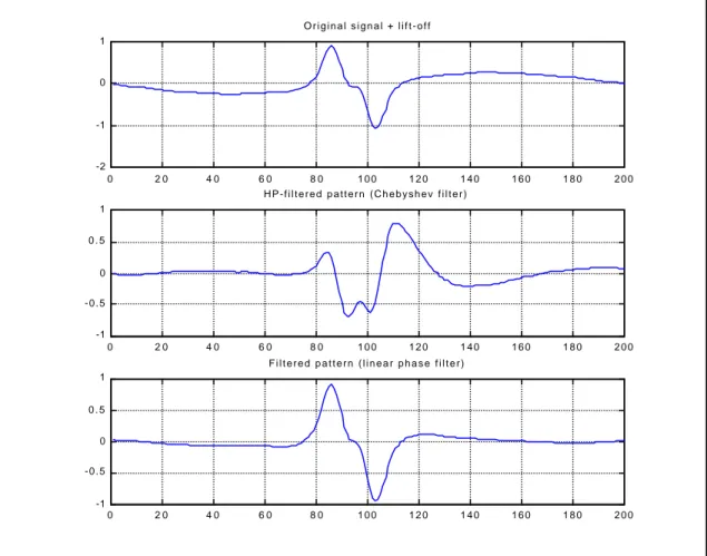
The In-phase and Quadrature components from the detectors are filtered to suppress a high frequency electronic noise and a low frequency lift-off signal. This latter operation which is commonly used to increase SNR by reducing the amplitude of the variable lift-off signal may cause a serious distortion of EC patterns if filtering is too “hard” and the filters introduce phase distortion.

We will illustrate this phenomenon by a numerical simulation. We will filter a real EC signal acquired from a differential transducer (KD pen-probe from ESR) sensing a small hole in an aluminum plate (the whole scan will be presented in the next section). To show the filtering effect we add a sine lift-off component with frequency two times lower than the main frequency of the EC pattern. The signal is then filtered by the fourth order high pass Chebyshev filter simulated in Matlab. Analog versions of this filter are commonly used as signal filters in EC instruments. Finally, we will filter the signal with a linear phase version of the Chebyshev filter also simulated in Matlab.

-1 -0.5 0 0.5 1 -1.5 -1 -0.5 0 0.5 1 Original pattern -1 -0.5 0 0.5 1 -1.5 -1 -0.5 0 0.5 1

Original pattern + lift-off

-1 -0.5 0 0.5 1 -1 -0.5 0 0.5 1

HP-filtered pattern (Chebyshev filter)

-1 -0.5 0 0.5 1 -1 -0.5 0 0.5 1

HP-filtered pattern (linear phase filter)

Figure 11a. Eddy current pattern from a differential probe filtered by HP filters

The results are shown in Fig. 11a and b which illustrates typical situation in mechanized ET, where the variable, low-frequency lift-off component limits the SNR. There is a

(19)

off but this difference is to small to suppress the lift-off completely. An obvious solution is to use a high pass filter with cut-off frequency just above the main frequency of the lift-off component. A pair of analog Chebyshev or Butterworth filters can do the job and they do (the lift-off component is reduced substantially, (see Fig 11b) but they also introduce distortion in EC pattern, as can be seen in Fig. 11a. The reason for this distortion is a nonlinear phase response of common analog filters. Different frequency components of the EC pattern are shifted differently by the filter and the typical result can be seen in Fig 11a, panel 3. The filtering effects sizing since it changes signal amplitude. It also makes any kind of more sophisticated signal analysis for defect characterization practically impossible.

0 2 0 4 0 6 0 8 0 1 0 0 1 2 0 1 4 0 1 6 0 1 8 0 2 0 0 -2 -1 0 1 O r i g i n a l s i g n a l + l i f t - o f f 0 2 0 4 0 6 0 8 0 1 0 0 1 2 0 1 4 0 1 6 0 1 8 0 2 0 0 -1 - 0 . 5 0 0 . 5 1 H P - f i l t e r e d p a t t e r n ( C h e b y s h e v f i l t e r ) 0 2 0 4 0 6 0 8 0 1 0 0 1 2 0 1 4 0 1 6 0 1 8 0 2 0 0 -1 - 0 . 5 0 0 . 5 1 F i l t e r e d p a t t e r n ( l i n e a r p h a s e f i l t e r )

Figure 11b. Quadrature component of eddy current patterns from Figure 11a.

The solution to this problem is using linear phase filters that do not introduce distortion in the signal (cf. Fig. 11a, panel 4). However, analog versions of such filters are complex and difficult to realize, therefore digital filters should be used for this purpose. Concluding, we will include the following variables to our list of essential variables: • Type of signal filters used in EC instrument

• Cut-off frequency of high-pass filters. We can recommend the following:

• Identify the filter type used in the instrument used for the ET inspection • Avoid hard filtering of EC signals

(20)

5. Probe resolution

Characteristics of the EC probe, such as its sensitivity to the expected defect type, internal balancing and spatial resolution are keys to the success of an ET inspection. Many probes for surface inspection are hand made, in the way based on manufacture’s know how and knowledge about the potential applications. Probe sensitivity and resolution is normally improved by introducing a kind of ferromagnetic core (often made of ferrite) concentrating magnetic flux. Probe windings are often wound by hand directly on the ferrite core. Cylindrical encircling coils for tube testing are manufactured using winding machines filling grooves in a plastic spool with copper wire. The spool geometry and number of windings govern coil characteristics. Because of the differences in manufacturing the surface probes exhibit quite large deviation of characteristics, each probe is an individual. Unfortunately, probe manufacturers very seldom provide users with more detailed data on probe characteristics enabling comparison of different probes. This means that the users should perform calibration of all probes to ensure that their parameters do not change over time. This is particularly important when replacing probes with their equivalents.

A good way of characterizing probes is measuring their response to a specific artificial discontinuity, for instance a drilled hole. Such response can be acquired using a computer controlled XY-scanner and an EC instrument. In Figure 12 below, we present examples of such responses acquired for three different probes manufactured by Rohman. The probes, excited with frequency 500 kHz, were scanned over an aluminum plate with a deep hole with a 1 mm diameter.

Figure 12a. Quadrature component of the response of an absolute probe KAS 4-3 to

(21)

Figure 12b. Quadrature component of the response of a differential probe KD2 to

a 1mm hole in an Al-plate. 3D presentation (left) and false color image (right).

Figure 12c. Quadrature component of the response of a differential probe KDF

76-3 to a 1 mm hole in an Al-plate. 76-3D presentation (left) and false color image (right).

The responses presented in Figure 12, often referred to as Point Spread Functions (PSF), provide important information about probe type, its spatial sensitivity and spatial resolution. Based on PSF we can also evaluate probe symmetry and predict its response to different discontinuities. For instance, probes KD and KDF (Fig. 12b and c) are both differential but have different sensitivity patterns. KDF is asymmetric and has lower resolution in vertical direction, which makes it suitable for detecting cracks. It can also detect small holes and pits but with lower sensitivity than the more focused KD. Generally, sensitivity patterns of differential probes are highly asymmetric, they have well pronounced sensitivity maximum in one direction. Absolute probes are insensitive to scanning direction but their response to a small defect depends on the location of this defect relative to probe center.

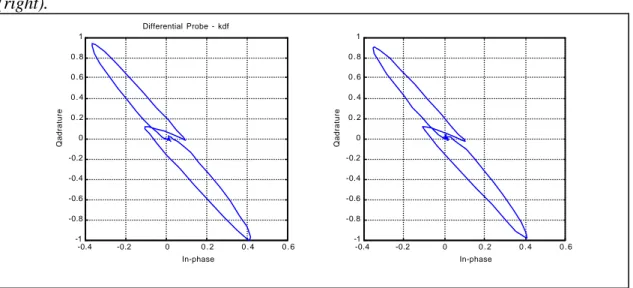
The distance of the detected defect from the probe center is a very important issue affecting both inspection sensitivity and defect sizing. This is illustrated by the examples shown in Fig. 13.

(22)

- 0 . 1 - 0 . 0 5 0 0 . 0 5 0.1 - 0 . 4 - 0 . 2 0 0.2 0.4 0.6 0.8 1 A b s o l u t P r o b e - k a s - 0 . 1 - 0 . 0 5 0 0 . 0 5 0.1 - 0 . 4 - 0 . 2 0 0.2 0.4 0.6 0.8 1 1.2

Figure 13a. Response of an absolute probe KAS 4-3 to a hole in Al plate. Maximum

sensitivity in the probe center (left) and the response 1 mm from the probe center (right). - 1 - 0 . 5 0 0.5 1 - 1 - 0 . 5 0 0.5 1 Differential Probe - kd I n - p h a s e Qadrature - 1 - 0 . 5 0 0.5 1 - 0 . 8 - 0 . 6 - 0 . 4 - 0 . 2 0 0.2 0.4 0.6 0.8 1 I n - p h a s e Qadrature

Figure 13b. Response of a differential probe KD2 to a hole in Al plate. Maximum

sensitivity in the probe center (left) and the response 1 mm from the probe center (right). -0.4 -0.2 0 0 . 2 0 . 4 0 . 6 -1 -0.8 -0.6 -0.4 -0.2 0 0 . 2 0 . 4 0 . 6 0 . 8 1 Differential Probe - kdf In-phase Qadrature -0.4 -0.2 0 0 . 2 0 . 4 0 . 6 -1 -0.8 -0.6 -0.4 -0.2 0 0 . 2 0 . 4 0 . 6 0 . 8 1 In-phase Qadrature

Figure 13c. Response of a differential probe KDF 76-3 to a hole in Al plate.

(23)

From Fig. 13 it can be seen that probe KDF due to its broad response is relatively insensitive to the location of small defects. The two other probes have steep responses and the amplitude of their responses to small defects is very sensitive to their distance from the probe center. This means that these probes require relatively high scanning density but are characterized by high spatial resolution and high sensitivity. It should be noted that the spatial responses of EC probes depend not only on their geometry but also to some degree on the test frequency.

Summarizing, we will include as an essential parameter

• PSF (point spread function) of the EC probe used for the inspection For successful EC inspection we also recommend:

• Periodical measurements of PSFs for all EC probes in use

• Considering PSF when selecting probes for a particular inspection

6. Characterizing EC patterns

In the proceeding sections we presented examples of different EC patterns for absolute and differential probes. From the theory and modeling of electromagnetic fields in ET context it appears that there are two main parameters characterizing EC responses in complex plane, amplitude and phase. However, these apparently simple parameters can be defined in many ways, giving slightly different results.

The most common way is choosing a point of the complex valued response that has maximum amplitude and taking its angle as a measure of phase. This seems reasonable for regular, symmetric, 8-like patterns, characteristic for differential coils used for tube testing. It can be much more difficult for asymmetric responses from absolute probes or especially for filtered responses of the type shown in Fig. 11a, panel 3.

Figure 14. Parameters of EC pattern used

(24)

Table 2. Parameters (features) used in Battelle study.

Feature Definitions Description

1 CHH Power in horizontal channel

2 CVV Power in vertical channel

3 CVV/CHH Ratio of power

4 √√CVVCHH Geometric mean of power

5 CHV/ √√CHHCVV Correlation

6 λ1 Maximum eigenvalue of the power matrix

7 λ2 Minimum eigenvalue of the power matrix

8 λ1 λ2 Product of eigenvalues

9 ∠λ1 Angle of eigenvector corresponding to the maximum

eigenvalue

10 (Hmax — Hmin)/√ CHH Horizontal voltage (peak-to-peak)

11 (Vmax — Vmin)/ √CVV Vertical voltage (peak-to-peak)

12 r Length of the radial vector

13 ∠ r Angle of the radial vector

14 … Area of Lissajous pattern above the horizontal axis

15 … Area of lower lobe of Lissajous pattern below the horizontal

axis

16 r1 Length of upper lobe

17 ∠r1 Angle of upper lobe

18 r2 Length of lower lobe

19 ∠ r2 Angle of lower lobe

20 ... Vertical-channel autocorrelation at Lag 40

23 ... Vertical-channel maximum frequency response

24 ... Vertical-channel frequency of maximum response

25 ... Vertical-channel total power

26 ... Vertical-channel first moment

27 ... Vertical-channel second moment

Other common ways, suitable for any type of patterns is choosing the phase angle that yields the best SNR in the component used as output (mostly the Qadrature).

There are many other ways of characterizing EC patterns (see, e.g., Doctor, et al, 1981, EPRI, 1998, Stepinski 1993 and 1994). As an example we present parameters used in a study performed by P.G. Doctor and coworkers at Battelle (Doctor et al, 1981) (cf. Fig. 14 and Table 2). The main aim of this study was investigating relevance of different parameters (features) commonly used in pattern recognition to classification of EC patterns (referred to as Lissajous patterns). Most of the proposed parameters appeared to be not very useful but the above list can serve as an illustration of the variety of parameters that can be used for describing EC patterns. The study did not give any definitive answer concerning relevance of the above mentioned features. The three features that contained most information using Fishers weighting as a relevance measure, were: #25 (vertical-channel total power), #8 (product eigenvalues), and #13 (angle radial vector). Other relevance criteria resulted in different features.

It is essential for the outcome of the test what parameters will be chosen, especially that different applications call for different parameters. For instance, when inspecting a material surface we can relay on the amplitude as a measure of defect size, while during detecting deeper subsurface defects the phase also has to be taken into account.

Precise definition of the chosen parameters becomes very essential for accurate sizing of detected defects. A small subsurface defect may result in a response similar to that of a

(25)

Summarizing we will include to the list of essential variables: • Parameters of EC patterns used for defect detection and sizing. We also recommend:

• Precise and unique definition of parameters

• Taking care when changing other parameters, such as, power of the feeding generator and filter settings, since they may change shape of the EC patterns

7. Lift-off

Variations in lift-off with an eddy current surface-scanning probe or wobble of an encircling coil for tube testing result from the unevenness of the object’s surface or mechanical vibrations of the scanner. It is well known from the theory that the variations of impedance components of an eddy current coil resulting from lift-off changes depend on the value of the normalized frequency fN, where fN = 2πf µσr02. Thus for a given frequency f and coil radius r0 the impedance variations depend on the product µσ of the magnetic permeability and the electrical conductivity of the test sample. In other words, the generalized impedance diagram is shifted with lift-off

Figure 15. Lift-off curves

obtained for a simple coil excited at frequency 500 kHz with balance in the air. Response to a slot with depth d in mm depends on the lift-off value h in mm.

changes and points corresponding to different fN are shifted differently. Blitz (1997) presents results of EC measurements of lift-off from a mild steel test block containing saw-cuts having different depths ranging from 0 to 10mm. He used a simple coil excited with a frequency of 500 kHz that was balanced, in each case, at “infinite” lift-off from the block and lowered to the surface, firstly at a defect-free region then, in turn, at the opening of each cut. Fig. 15 shows how amplitude of the responses from the saw-cuts depends on the value of lift-off if the lift-off value h is increased from zero to a maximum value of 5 mm. Thus, to evaluate crack depths in a sample made from a material identical to that of the test block, calibration curves plotted for slots of different depths at the desired frequency of operation should be used.

Similar curves should be plotted for all types of probe−material combinations and used for defect sizing. It should be noted that the above example illustrates detection of surface breaking cracks only. For subsurface defect the situation is more complicated since phase variations cannot be neglected.

(26)

Summarizing we can note that lift-off variations not only decrease SNR but also affect amplitudes of EC responses. Thus, lift-off should be considered as a parameter essential for the inspection especially during defect sizing.

8. Defect orientation

It is obvious that defect orientation influences EC response and its sizing. Although this factor will not be considered here, for completeness of this report we present an example illustrating how the orientation of subsurface crack may change the EC response of a simple absolute coil ( Blitz, 1997).

Figure 16. Coil responses to cracks

with different orientation.

Generally, geometry of a particular defect influences the EC response in the way specific for probe type. It should be mentioned that EC probes are defect direction sensitive, for instance, a simple coil is insensitive to the flat subsurface flaws parallel to the inspected surface. Thus, defect orientation should be definitely placed on the list of essential variables.

(27)

9. Conclusions

We have considered a number of variables that may influence the outcome of ET. Most of the analyzed variables were related to the internal structure of EC instrument. This analysis is important because the user normally does not have much insight into the EC instrument he uses and has to rely on its performance. However, some instrument parameters that are essential for the test may be controlled by the user, for example, nonlinear distortion in the pick-up or filter settings. Therefore the user should have enough knowledge to choose the correct settings and to notice and avoid malfunction of the EC instrument.

We have motivated placing the following factors on the list of essential parameters:

EC Instrument Function Essential Variable

Probe • Probe unbalance signal (for internally balanced

probes) • Probe lift-off

• Probe PSF (Point Spread Function - 2D response) Input circuit • Type of balancing circuit

Detector • Amount of harmonic distortion in the carrier signal • Detector type

Filters • Type of signal filters used in EC instrument • Cut-off frequency of high-pass filters.

Signal characterization • Parameters of EC patterns used for defect detection and sizing

As mentioned in the Introduction this is a preliminary study indicating some selected variables essential for ET. However, many important issues, such as the effect of defect orientation, the optimal use of probe resolution or characterization of EC patterns remain unsolved.

(28)

10. References

ASM Handbook, Vol 17, Nondestructive Evaluation and Quality Control, Eddy Current

Inspection, ASM 1996.

J. Blitz, Electric and magnetic methods of NDT, Chapman & Hall, 1997.

ENIQ Recommended Practice 3: Strategy Documents for Technical Justification, ENIQ

Report nr.5, EUR 18100EN, EC, DG-Joint Research Centre, Petten Site, July 1998. P.G. Doctor, T.P. Harrington, T.J. Davis, C.J. Morris, and D.W. Fraley, Pattern Recognition Methods for Classifying and Sizing Flaws Using Eddy-Current Data in

Eddy Current Characterization of Materials and Structures, Birnbaum & Free, editors,

American Society for Testing and Materials, 1981.

H. Libby, Introduction to Electromagnetic NDT Methods, Robert Krieger Publ. Company, 1979.

EPRI, Steam Generator Automated Eddy Current Data Analysis, A Benchmark Study, Report TR-111463, December 1998.

NDT Handbook, Vol 4, Electromagnetic Testing, R.C. McMaster, editor, ASNT, 1986.

T. Stepinski and N. Masszi, Conjugate Spectrum Filters for Eddy Current Processing, Materials Evaluation, vol. 51, no 7, 1993, pp. 839-844.

T. Stepinski, Digital Processing of Eddy Current Signals and Images, Proc of the 6th European Conf. on NDT, Nice, October 1994, pp. 51-55.