Storage Efficient Code on Microcontrollers

Faculty of Technology and Society Department of Computer Science and Media Technology

Bachelor’s Thesis

15 credits

Storage Efficient Code on Microcontrollers

Lagringseffektiv Kod p˚a Mikrokontrollers

Hampus T˚

agerud

Degree: Bachelor of Science, 180 credits Major: Computer Science

Specialisation: Computer Systems Development Date of Opposition Seminar: 30 May 2018

Supervisor: Gion Koch Svedberg Examiner: Farid Naisan

Bachelor’s Thesis 2018

Department of

Computer Science and Media Technology

Malm¨o University 205 06 Malm¨o Sweden https://www.mau.se c Hampus T˚agerud, 2018 Typeset using

L

A

_TEX

Abstract

In this paper, a more storage efficient way of running code on microcontrollers is presented, implemented and compared against the conventional method. The method involves utilising a jump table and the objective is to be able to execute larger amounts of code than fits into the program memory of the microcontroller. Without loosing too much performance.

In conclusion, there is no obvious answer to whether the implemented system is a viable alternative to traditional applications or not. More variables than just performance are brought up and must be considered when a system is implemen-ted. However, the developed prototype introduced a minor overhead of about 1%. It could therefore be concluded that the prototype is a viable alternative, to the conventional way of running applications, performance-wise.

Sammanfattning

I den h¨ar rapporten presenteras och implementeras ett mer lagringseffektivt s¨att att k¨ora kod p˚a mikrokontrollers. Det j¨amf¨ors ocks˚a med det traditionella s¨attet detta g¨ors p˚a. Metoden involverar en hopptabell och m˚alet ¨ar att kunna k¨ora st¨orre m¨angder kod ¨an vad som kan lagras p˚a mikrokontrollern. Utan att f¨orlora f¨or mycket prestanda.

I slut¨andan finns det inget sj¨alvklart svar p˚a om systemet som implementerats ¨ar ett bra alternativ till traditionella applikationer. Fler faktorer ¨an bara prestanda presenteras och m˚aste beaktas n¨ar system implementeras. Den utvecklade proto-typen introducerade en overhead p˚a cirka 1%. D¨arf¨or kunde slutsatsen dras att prototypen ¨ar ett rimligt alternativ (prestandam¨assigt) till det traditionella s¨attet att k¨ora applikationer.

Acknowledgements

I would like to thank my supervisor, Gion Koch Svedberg, for his help during this project. Not only did he provide me with valuable help, feedback, suggestions and ideas but he did so with a genuine interest.

I also want to take the opportunity to thank friends and family that encouraged and pushed me forwards. An extra thank you goes out to my beloved parents who, through my entire childhood, tried to drag me away from computers. Fruitless attempts that only increased my interest in learning more about it.

Table of Contents

1.2.3 Efficient Storage Usage . . . 8

1.3 Research Question . . . 9

1.4 Scope . . . 9

2 Related Work 10 2.1 Java . . . 10

2.1.1 Software . . . 11

2.1.1.1 Tiny Virtual Machines . . . 11

2.1.2 Hardware . . . 12

2.1.2.1 Running Code . . . 12

2.1.2.2 Loading Code . . . 13

2.2 Script Interpreters . . . 13

2.3.1 Dynamic Linking . . . 14

2.3.2 RETOS . . . 14

2.4 Relation . . . 14

3 Method 16 3.1 Design and Creation . . . 16

3.2 Experiment . . . 16 3.3 Alternative Methods . . . 17 4 Implementation 18 4.1 Tools . . . 18 4.2 Solution . . . 19 4.2.1 Base System . . . 19 4.2.2 Jump Table . . . 20 4.2.3 Loadable Code . . . 21

4.2.4 Loading and Executing . . . 21

5 Experiment 23 5.1 Overview . . . 23 5.2 Equipment . . . 25 5.3 Measurement . . . 26 5.3.1 Emulated Hardware . . . 26 5.3.2 Physical Hardware . . . 26 6 Results 28 6.1 Execution times . . . 28 6.2 Code Size . . . 30 7 Discussion 32 7.1 Emulated Hardware . . . 32 7.2 Overhead . . . 33 7.2.1 Performance . . . 33 7.2.2 Code Size . . . 34

7.3 Considerations . . . 34 7.3.1 Application Development . . . 34 7.3.2 Security . . . 35 7.3.3 Reliability . . . 35 8 Summary 36 8.1 Conclusion . . . 36 8.2 Future Work . . . 37 8.3 Summary . . . 37 References 39

1

Introduction

Microcontrollers are small, cheap computers where all the parts have been embedded into a single package. They are an important part of today’s society and, with the recent rise of the Internet of Things (IoT) technology, the demand for microcontrollers will only increase tremendously. The uses of microcontrollers are endless, from residing in devices on our wrists to controlling our cars, they are everywhere. However, compared to most modern computers, microcontrollers are very limited both when it comes to memory, stor-age and processing capabilities. This study focuses on the limitation of storstor-age memory. A system, that aims to improve developer’s flexibility, is developed and compared against the traditional way of running code on microcontrollers. Many situations, where micro-controllers are applicable, do not require high processing power but they occupy a lot of storage memory. Working around this limitation, of some cheaper microcontrollers, could allow for cheaper devices to be developed where the amount of memory is more important than the processing capabilities.

1.1

Background Theory

Microcontrollers are integrated circuits1 that house a complete computer system, which is why they were originally called microcomputers before it was changed to microcontroller [2]. It holds a combination of electrical circuits providing it with memory2for programs and data, a processing unit for executing instructions and peripherals for communication with

1

An integrated circuit (IC or chip) is a thin sheet of semiconducting material, normally silicon, and contains all components and wiring of an electronic circuit on its surface. [1].

2

FLASH memory is used for storage and SRAM is used for data [2]. SRAM is faster but volatile, meaning that the data only persists while the circuit is powered. FLASH is non-volatile but is slower and have a shorter lifespan than SRAM.

1. Introduction

other circuits or devices. At its core is a processing unit referred to as an ALU (Arithmetic Logic Unit) which allows the microcontroller to fetch and execute instructions [2]. These instructions are stored in memory and accessed, at runtime, by the logic unit. The ALU then fetches a desired instruction, interprets it and changes the state of the microcontroller accordingly before it starts over. This is known as the ALU executing a cycle and it is what is being referred to when a processor is said to have a speed of a certain amount of MHz or GHz [1]. These numbers are telling how many cycles a processor is able to perform each second.

In order to make the microcontroller useful, it needs to be able to transfer data into and out of itself. This could be as simple data as turning on a light bulb to more complex tasks like writing on a display or transmitting data over a network connection. When the microcontroller’s state changes it is sending different combinations of electrical sig-nals which can be interpreted by other hardware [2]. Likewise, the microcontroller itself may be configured into reading and interpreting electrical signals from other hardware components. This is the way all our current computers work, different scales but same principles.

Microcontrollers also execute interrupts [2]. Interrupts are very aptly named because they are basically interrupting the currently executing code. This is being done by the processor listening for interrupt calls after each instruction that has been executed [3]. If an interrupt request is detected the microcontroller will stop the execution and then jump into an interrupt handler, which will execute new code [2]. When everything is handled, the microcontroller will jump back into the code it executed before the interrupt. The processor listens to these interrupt requests on a different channel than the other data flows and can, therefore, stop the general execution and then jump back into it when the interrupt handling is finished [2].

The primary use of a microcontroller is to build embedded systems (systems that are de-signed to serve few, highly specialized purposes), unlike general-computing devices which can be repurposed to perform any computable task [4]. It comes without any software installed (except for the occasional bootloader installed to ease uploading new software) which means that developers must install their own program before any computations are actually performed by the device [2]. This installation is performed by uploading the soft-ware into the memory of the microcontroller. The devices needed to upload the softsoft-ware are different depending on the microcontroller being programmed. Traditionally vendor specific hardware has been required in order to upload new software to microcontrollers. However, recently manufacturers have started to implement USB support into their

mi-1.1 Background Theory

crocontrollers which enables developers to upload software with a standard USB cable. Whether the microcontroller can be programmed over USB or not there is still a need for software to be running on the development computer. The role of this software is to communicate with the microcontroller, through the chosen interface, and upload the new code.

1.1.2 Computer Architectures

The components of a computer can be arranged in different ways, called an architecture or computer configuration and there are two commonly used architectures today [2]. The first one is called the Harvard architecture and the second one is known as the Von Neumann architecture. How they differ boils down to how they manage their respective memory modules and inputs. As mentioned earlier a computer needs memory for storing program instructions and data (variables created by the software at runtime). The Harvard architecture uses separate modules for each purpose. This means that a computer based on this configuration has one memory module for the program instructions and one for the data produced [2]. The ALU can access both these memory modules and its input/output peripherals simultaneously through separate buses1 which can speed up overall execution speed.

The Von Neumann architecture is using a different approach by implementing a single bus to access both data and instruction memory [2]. Why this matters is mainly because most of the time when the processor is going to execute an instruction it is going to need more information. Data might be created dynamically at runtime and then stored as data. Applications are loaded into memory from storage when they are executed and unloaded when they are not running any more, unlike the Harvard architecture where the code is statically stored in the FLASH memory. Accessing this data with a Von Neumann configured computer is requiring the execution of the program to halt for a certain amount of cycles while the processor fetches the information required. A computer based on the Harvard architecture, however, is able to fetch the data while executing the program. Meaning that the processor will not stop the execution in the same way [2]. This limit imposed on the Von Neumann architecture is called the ”Von Neumann bottleneck” and refers to the fact that the performance of the computer is limited due to the way it is

1_{A bus is a set of wires that connect one or more electronic devices and allows communication between}

them [1]. Using messages, specified by a defined protocol, the connected devices can send and receive information over this communications line in the form of electronic voltages that must be interpreted [3].

1. Introduction

designed. Processing speeds today are so high, though, that this does not pose a significant problem which has led to Von Neumann being the most widely used computer architecture today seeing how it is a simpler system to implement [2]. However, microcontrollers tend to be based on the Harvard architecture since it leads to higher processing speed thanks to being able to fetch instructions and data simultaneously [2].

1.1.3 Code Lifecycle

Computers and electronic devices understand 1’s and 0’s, known as bits [1]. When series of these are combined they are called bytes and are used to represent information in electronics. It can be miscellaneous data including the instructions that a computer should execute. This way of representing information is incomprehensible to us humans which is why high-level programming languages were invented [1]. These are written languages that are similar to our real written languages but they are easier for humans to develop software with.

Since computers do not understand human languages the source code developers write needs to be translated into a big chunk of 1’s and 0’s (a binary). The process of doing this translation is called compilation [1]. A compiler is a computer program that takes source code in a human-readable format as input and outputs binary files with machine code that computers can process [1]. When the compiler has finished a linker needs to be invoked. It assembles all produced machine code into a single executable file and ensures that all the pieces are connected [5].

When a binary file has been produced, the final step is to get it onto a microcontroller (uploading it into the circuit). Using the hardware and software needed to do this, the code is being burned into the program memory of the microcontroller [6].

1.1.4 Linking Methods

Linking the generated machine code is the last step of the compilation process [5]. By examining the code to be linked the linker can deduce how to fit them together and then connect them. Connecting pieces of code means inserting addresses to which the execution should jump in order to continue the execution of another piece of code[3].

There are two approaches to linking pieces of code together, static and dynamic [3]. The difference is most often not visible to the end user but can affect developers in a variety of ways. Static linking specifies that the linker inserts fixed addresses into the executable code. The linker has access to all parts being linked and can, therefore, calculate exactly

1.1 Background Theory

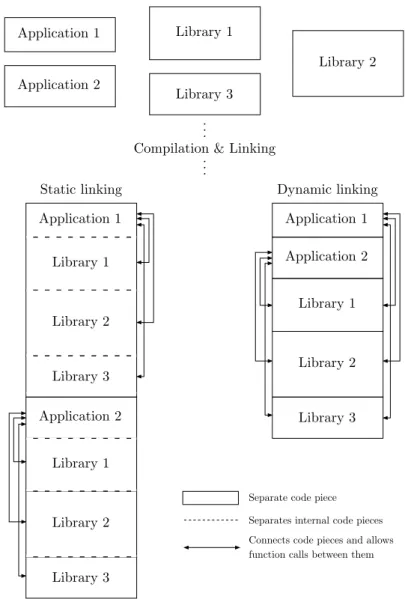
how to fit them together [3]. This infers that the final binary is not modifiable1, it is static. The resulting binary also includes the codes of linked libraries inside itself [5]. On the other hand, dynamic linking inserts reference addresses when linking the code, enabling a system to set these addresses at runtime instead [5]. This allows parts of the application to change even after it has been built. Using this technique permits a system to reuse code between different applications by setting their relative addresses to the same memory locations [5]. Say that a system has two applications that all use the same, heavy code library. Instead of loading this library two times the system can have all applications use the same code, from the library, and thereby save memory and loading time. Loading and unloading is, however, a functionality built into operating systems (i.e. not available on microcontrollers by default) [3].

As seen in Figure 1.1, dynamic linking results in less memory usage since the libraries only have to be loaded a single time. Also, storing the binaries requires less space for the same reason. Therefore it can be concluded that if using dynamic linking a higher number of applications are able to fit in the very limited memory of a microcontroller.

1

Modifiable in the sense that the pieces can be moved and relinked. It is still possible to change the actual bytes of the binary.

1. Introduction Application 1 Application 2 Library 1 Library 2 Library 3 . . .

Compilation & Linking . . . Application 1 Application 2 Library 1 Library 2 Library 3 Library 1 Library 2 Library 3 Application 1 Application 2 Library 1 Library 2 Library 3 Static linking Dynamic linking

Separate code piece Separates internal code pieces Connects code pieces and allows function calls between them

Figure 1.1: Showing resulting binary applications from the dif-ferent linking techniques

1.1.5 Bootloaders

A microcontroller always starts its execution at a fixed position in its memory [7]. This is where uploaded code should be placed so it is always executed properly. Since the uploading of code might be a tedious process, sometimes even requiring special cables, a bootloader can be used to simplify the uploading [8]. A bootloader is a small piece of code that runs before the uploaded code. It is placed in the memory spot where the microcontroller goes to start its execution [3]. From there it can enable uploading new code using USB, Bluetooth, wifi or whatever technique that is appropriate for the device [7]. The bootloader is then able to receive and program code updates or execute stored

1.2 Problem Formulation

code if there is no updates available.

1.2

Problem Formulation

Low-end microcontrollers are cheap1 and small2 but not as powerful as their larger, more expensive alternatives. A major disadvantage is the limit imposed by small FLASH memory that can only store small pieces of code. However, with a system supporting loading code while the microcontroller is running, the memory can be used more effi-ciently. By being able to load and unload pieces of code a larger system can be split into any number of smaller parts. They can then be executed one by one. Adding external memory could seem like a solution but even if using external memory is supported by the microcontroller (which is false for many low-end devices) there would be a significant performance hit compared to the built-in memory. Although, given how cheap memory modules are, for example in the form of SD (Secure Digital) cards, an enormous amount of tiny code pieces can be stored and then loaded by the circuit. This would result in a longer loading time of the code but the execution speed would be faster since the built-in memory would be utilised instead.

Building products with microcontrollers requires several variables to be considered when selecting a circuit to base the system on. Even though a cheaper microcontroller provides enough speed and amount of memory, if the code is too large to fit into the FLASH memory, developers will have to opt for a larger (more expensive) microcontroller. However, by only loading the required code, this could be avoided and the cheaper microcontroller would still be usable. It could mean reduced costs of both development and production while resulting in a smaller, lighter and more energy efficient product. It could lead to cheaper lines of products allowing more people to enjoy the technology. Also, IoT products could benefit from the technology, allowing them to be smaller and lighter while enabling updating firmware and the addition of features automatically during runtime.

1_{eBay has listings, of appropriate microcontrollers, with prices as low as $1.3 / 11.34 SEK [9].} 2

1. Introduction

1.2.2 Low-end Microcontrollers

Microcontrollers are a broad family of devices. Ranging from tiny circuits, for performing simple tasks, to large components, capable of running full-fledged operating systems, there needs to be a definition in place. In order to limit the scope of the study, and putting it into a context, we are limiting this study to low-end microcontrollers. Low-end refers to families of microcontrollers with limited hardware specifications and we are defining the limits to be:

Microprocessor Maximum 80MHz (S)RAM Maximum of 20kB

FLASH Maximum of 80kB

Devices conforming to these limitations are not only unable to run any modern operating systems. They are, therefore, unable to load and unload dynamically linked code. As will be later presented, there are existing solutions but they require more memory or higher clock speeds than is available on low-end devices.

1.2.3 Efficient Storage Usage

The interest of this study is to explore an efficient way of using the storage memory on low-end microcontrollers. By loading code, stored outside of the microcontroller, only when it is needed can enable larger amounts of code (than what fits in the microcontrollers storage) to be executed. A model of execution will be hypothesised, and later implemented, which aims to be more storage efficient.

Dynamic linking allows pieces of code to share their functions and variables with each other. However, on a limited system (such as low-end microcontrollers) the hardware is not able to facilitate such functionality of advanced operating systems. Therefore, it will be necessary to provide another solution with the same end result. This trait is still desirable, in order to reduce storage needed.

Code native to the hardware requires no additional steps to be executed. Opposite to this are solutions like virtual machines or interpreters. However, systems like these require extra code for the actual implementation which creates performance overhead and extra storage requirements. In order to make the solution as effective as possible, it should be utilising native code.

1.3 Research Question

The hypothesised solution is a system which loads code only when it is needed. It also allows code pieces to utilise code outside of themselves. The model is implemented in native code in order to minimise overhead, in terms of storage and execution time. By loading code only when it is needed and then unloading it enables large amounts of code to be split into several smaller pieces. These can be fitted in the memory of a cheap microcontroller with external memory instead of a more expensive with enough space for the entire application. The system will require extra code, to handle the loading and unloading of external code, which will create an overhead that will be measured. The resulting overhead can then be used to determine whether the solution is a viable alternative to traditional applications or not.

1.3

Research Question

Given the way the problem of this study has previously been described the research ques-tion (RQ1) is defined in the following way:

What kind of overhead follows with a more storage efficient system? Is this system a viable alternative to the traditional way of running code on low-end microcontrollers?

In order to be able to test the proposed solution there needs to be a system that implements it. Therefore a second research question (RQ2) is defined as:

How can a system be implemented, on low-end microcontrollers in native code, that uses storage more efficiently?

1.4

Scope

These research questions aim to limit the scope of the study enough to keep it from becoming too wide. They define that more capable hardware systems, such as Raspberry Pi and similar system-on-a-chip, are not included in the scope. They have too much resources to be considered to be low on resources. Such systems are also capable of running more or less full-fledged operating systems which in this case would defeat the entire purpose of this thesis.

It is also defined that the approach should run native code and thereby we are exclud-ing techniques such as virtual machines and interpreters. This is an area that is more researched and outside of the scope of this study.

2

Related Work

Microcontrollers were created to be part of very static, embedded systems and it seems like not a lot of research on breaking this pattern exists. Most of the articles show that the most popular solution to implement is a custom Java Virtual Machine. Java was launched as a ”write once, run everywhere” solution [11] so the choice, to implement it on microcontrollers, makes sense. It is a wide-spread language that is easy to pick up thanks to its many similarities to C and its derivatives. A problem is that the JVM (Java Virtual Machine) is taking up a lot of memory. It requires hundreds of megabytes of RAM, on desktop computers, and the standard library is also a huge pile of code. There exist subsets of Java that are smaller but do not implement the entire language. This makes for an interesting problem when it comes to microcontrollers since high enough hardware specifications, to enable the use of full Java, are hard to find.

When it comes to other alternatives some scripting engines and native solutions were also found. Research articles for these solutions were sparser than the ones about Java implementations but they show that there is some interest in other solutions than Java as well.

2.1

Java

As mentioned earlier, Java (in its conventional, full form) is not suited to be running on microcontrollers. Due to the way virtual machines and interpreted languages work, there is a requirement for a lot of memory. They have a lot of code running, just to execute applications, which consumes a lot of memory. Microcontrollers do not, typically, provide this much memory. However, there have been several attempts at realizing Java for microcontrollers.

2.1 Java

2.1.1 Software

In the results, of our database searches, papers on various Java Virtual Machines and other ways of implementing Java could be found.

2.1.1.1 Tiny Virtual Machines

The idea of having a JVM running on a microcontroller is a very nice one. Being able to write the software once and then be able to run it on any hardware would save any developer a lot of headaches. The problem when trying to implement it on microcontrollers is the hardware limitations, whatever solution chosen there is always going to be limitations imposed upon it which we will discover soon.

Darjeeling, for example, is an open source virtual machine made specifically for hardware lacking the huge amounts of memory Java needs [12]. It is based on a 16-bit architecture, instead of the standard 32-bit that Oracles JVM uses. Darjeeling targets 8 and 16-bit microcontrollers with less than 10kB of RAM and therefore the 16-bit approach is more sensible. It is the reason for the low hardware requirements, using a 16-bit instead of 32-bit architecture saves a lot of memory overhead. Enabling the 16-bit instruction set requires that the Java bytecode is being translated to custom instructions since the original Java code is in 32-bits. However, all this is handled by Darjeeling before execution. Even though it has low hardware requirements the virtual machine is able to implement a substantial subset of Java but it lacks certain features like reflection, synchronised, static methods and 64-bit data types. Object orientation is supported though.

Continuing in the same spirit, simpleRTJ is also a tiny VM running a subset of the Java language [13]. It is implemented in less than 20kB of code memory, enabling usage on very resource-limited microcontrollers. It does, however, require 18-23kB of RAM. This is something not all microcontrollers can boast about, making simpleRTJ a little less universally compatible with low-end microcontrollers’ specifications. Supporting excep-tions and events, it is an interesting option for developers looking to run Java on their microcontrollers.

Another study focuses on running Java on tiny sensors [14]. The project aims to abstract the underlying hardware to enable portable applications for sensors. The runtime acts as an operating system, being responsible for scheduling, loading Java classes, memory management and allowing interaction between Java applications and the hardware. Limits imposed on the system comes from the small code space available. Applications cannot be larger than 1022 Bytes, a requirement possibly hard to meet. Further limitations are no

2. Related Work

multi-threading, exceptions and only integers, bytes and chars can be manipulated. There is support for object-oriented programming with classes though.

2.1.2 Hardware

While building and installing a custom virtual machine on a microcontroller might seem like the most obvious solution, to implement Java, there has actually been (successful) attempts at making Java supported on hardware level [15]. Much like Apple has its ecosystem (where both hardware and software are under strict control) designing a system with both the hardware in mind, just as much as the software, is an approach that could potentially lead to greater success than just focusing on implementing the software.

The Komodo project [15, 16] aims to do just this. Its goal is to create a Java microcontrol-ler, with a JavaVM, that is able to run Java whilst being able to provide timing security identical to conventional C/C++ applications. Being able to ensure the timing, of the processor in the microcontroller, is crucial for real-time applications where the cycles of a processing unit must be countably handled in a predictable fashion [15]. Otherwise dead-lines in the applications can be missed which is unacceptable if it is a real-time application. Java is not an obvious choice in these contexts since it has several features running in the background (e.g. garbage collection) that cannot be controlled by the developer. If it is not a predictable behaviour than it is impossible for the developers to calculate, develop and test real-time applications.

2.1.2.1 Running Code

The microcontroller, used for the Komodo project, is a multithreaded Java microcontrol-ler. This means a microcontroller running several threads and actually able to execute some Java bytecode natively in the processor. This means that already the Komodo micro-controller has an advantage over pure software solutions since Java code can be executed just as fast as native machine code [15]. A custom virtual machine is running inside the microcontroller. Its responsibilities include loading the Java classes and interpreting the bytecode. It might seem like an unnecessary step to interpret code that can be run natively but there is a clever reason. Conventional Java VMs interpret bytecode and compile it to machine code native to the underlying architecture. What the VM in Komodo can do (running a Java microcontroller) is skipping the compile step and just pass the bytecode instruction to the hardware which can have impressive performance benefits [15].

On the problem of real-time applications, the researchers behind Komodo have taken advantage of the fact that they are running a multithreaded microcontroller. By letting

2.2 Script Interpreters

the running application occupy one thread and forcing all other features (scheduling, garbage collecting, interrupts etc.) into the other threads, the execution of the application becomes predictable and no other features can interfere.

2.1.2.2 Loading Code

Running a VM that handles the bytecode allows dynamic loading and unloading of Java classes [16]. Thanks to the multiple threads in the microcontroller, a class can be loaded in a separate thread and therefore without interrupting the execution of the already running applications. The class loading thread is able to load code from a class file and link it into the already loaded system. This approach, however, has its limitations. The number of threads on the microcontroller is limited and therefore only one class can be loaded at one point. This makes mutual dependencies impossible, two classes being loaded cannot de-pend on each other since loading and linking them is not possible. However, dede-pendencies in the form of polymorphism and uni-directional dependencies are still possible.

2.2

Script Interpreters

Two scripting engines were found during the literature review, JerryScript and Tapper. JerryScript is an engine enabling JavaScript for microcontrollers with less than 64kB RAM and less than 200kB program memory [17]. It is ECMA1 _{compliant and therefore}

comfortable for any JavaScript developer to get started with. It also provides access to the devices’ peripherals, making JerryScript suitable for IoT solutions (JerryScript powers the IoT.js project) where small microcontrollers need to interact over the internet, the place ruled by JavaScript.

Tapper is another scripting engine claiming to be very lightweight and trying to change the way developers think about embedded development [18]. Instead of developing applic-ations for single chips, the developers want to provide a platform to run portable, scripted applications upon. It is able to run on as a bare-metal2 application and uses 3-11kB of program memory and just 230B to 1.5kB of data memory. Being one of the lightest systems presented in this literature review, Tapper is an impressive system. Writing scrip-ted applications abstracts some system development that C or C++ would require which

1

ECMAScript is a standard created by Ecma International to govern JavaScript implementations.

2

Bare-metal indicates that the code is running directly on the processor without any operating system (or similar solution) between the code and the hardware.

2. Related Work

is interesting from a productivity perspective. The paper claims that Tapper offers the best compromise between performance, overhead, code size and portability. Regarding overhead, it is being described that it takes between 20-3000 cycles to execute a com-mand depending on complexity. Code examples are not shared in the paper to describe complexity of the commands, requiring higher amounts of cycles, but it can be deducted from the paper that those commands would require high amounts of cycles in conventional applications as well.

2.3

Native

2.3.1 Dynamic Linking

In order to be able to provide over-the-air update, dynamic linking is proposed to enable better software for IoT devices [19]. The system is based on the FreeRTOS (Real Time Operating System) software which is providing an operating system for microcontrollers (open source). The framework can load an application, link it to FreeRTOS and then execute it via a FreeRTOS task. The data shows a slight overhead from loading and linking applications, however after the application is started there is no more measurements. It is claimed to be the same performance as native applications, as long as the application does not communicate with the system, but no data is provided.

2.3.2 RETOS

RETOS is an operating system for microcontrollers able to reconfigure itself by loading and unloading kernel modules [20]. It was built as a sensor network OS with the objectives to provide a robust, reconfigurable and multithreading operating system. It uses a dual stack system, meaning that there is one stack for user applications and one stack for the kernel and operating system. The reconfiguring of the system is achieved by constantly loading and unloading kernel modules. When loading the modules (stored in a custom format) the code is loaded and linked based on the meta-info in the stored executable.

2.4

Relation

The idea of loading and unloading code is not new but still not widespread on microcontrol-lers, due to the limited hardware they feature. Earlier, virtual machines and interpreters have been used to implement the ability to accomplish this. However, they do also come with a significant overhead since they need to set up and host an environment inside which

2.4 Relation

the code will run. This is how the proposed solution will stand out, it does not need a wrapper environment or any other system between the code and the software. Once the code is loaded and starts its execution, it is running directly on the processor. To enable code reuse, like dynamic linking does, in native code the processor has to jump between the executing code and the piece of code that contains the desired function. Requiring the processor to jump between firmware and loaded code, to perform actions and pass data, will create an overhead. How big this overhead is hard to define before testing a system implementing this, which is why this study is performed.

3

Method

The research question asks how much overhead is created by not running code immediately. Due to the quantitative nature, of this question, there is a need to collect quantitative data in order to answer it. This will be done by performing an experiment that will test and compare how well traditional code perform against the solution created.

3.1

Design and Creation

Designing artefacts is a popular research method in the computer science field [21]. The output of Design and Creation can be theoretical and/or practical. The method aims, typically, to solve problems through an iterative process [21]. A prototype is created and then slightly modified until the implementation is satisfactory based on the research question.

An example of Design and Creation is a research project that compares and evaluates two development methods, constructs or models [21]. This is appropriate to answer the second research question, RQ2. A system, that implements the hypothesised solution, can be created and compared against the conventional way code executes on microcontrollers. From the resulting data an attempt to answer the first research question, RQ1, can be made.

3.2

Experiment

It is common that a second research method is used along with Design and Creation (in order to evaluate the outcome of the research) [21]. In the case of this study an experiment will be used to evaluate the created system. Most experiments have both dependent and independent variables [22]. Variables are classified based on how they interact upon chan-ging. Independent variables are not changed based on how a dependent variable changes while a dependent variable is affected by how an independent variable is changed. They

3.3 Alternative Methods

can be thought of input/stimulus (independent variables) or output/response (dependent variables) [22]. The objective, when performing an experiment, is to measure the impact a change of independent variables causes on dependent ones [22]. This is being made by creating a situation and then manipulating it, similar to case studies [23].

There exist different kinds of experiments, field-experiments and controlled experiments [24]. Field-experiments involve creating a situation in real life, then changing some vari-ables and observe how the situation changes. It works a lot like case studies but involves studying a larger population, large enough to be scaled and still applicable to the general population [24]. However, since field-experiments are taking place in the real world, it may be contaminated by variables and factors not introduced by the researcher but pre-existing in the world [24]. Controlled experiments are different because the entire situation, and its environment, is created by the researcher which allows complete control over all variables [24]. All unwanted variables can be excluded, allowing only the variables of interest (to the research) to be studied [21].

This study creates a controlled experiment to test the system designed and conventional code for microcontrollers. The data acquired from the experiment will be used to compare the different models of running code and evaluate the efficiency of the created solution, which is intended to answer RQ1.

3.3

Alternative Methods

Qualitative methods, such as interviews and case studies, are not suitable for this kind of research since the primary research question is quantitative in nature. The data wanted (in this case execution times of different pieces of code) can only be acquired by actually running the code and time it. An experiment can also be considered the proper method since it provides an unbiased result and can be controlled in every way [21].

In order to create and perform the experiment, a system to test is needed and this is where the Design and Creation research method fits. A system, satisfying the hypothesis, needs to be implemented and this can only be achieved by designing and creating it. The only argument against this would be to utilise an existing solution which, as mentioned in the previous chapter, was not found.

4

Implementation

This section is dedicated to the system created to implement the hypothesised solution. The concepts used during development will be presented and explained in order to provide an understanding of the internal workings, enabling reproducibility of the design.

4.1

Tools

The arm-none-eabi toolchain is used to compile the software. This is a set of tools, based on the GNU Compiler Collection (GCC), that the company ARM develop themselves and provide to developers developing for ARM-microcontrollers. The toolchain is open-source and therefore free of charge. By defining that GCC is being used it is also implied that the system is being built with a language supported by the compiler collection. For this project C is used but it is worth mentioning that also C++ and Assembly would be available to be utilised, these are all languages supported by ARM. Creating and compiling the source code is set up like a standard project for the C language would be. Any text editor or IDE (Integrated Development Environment) can edit the text files and the toolchain is able to compile everything manually. A build system like CMake1or Meson2 greatly eases the process of building the application and is therefore recommended. The GCC is also useful for the purpose thanks to a included linker program that allows defining, in a very customisable manner, how the loadable code should be linked. The linker also enables defining memory locations/limits and other options that will prove useful when developing the system later.

As described before, the system is being implemented in the C language. Not only is it one of the most used languages for developing microcontroller applications but it also has some important features needed to develop the system. The most important of these are the

1_{https://cmake.org} 2

4.2 Solution

ability to define functions and then being able to create pointers1 pointing towards these functions. Function pointers are the way loaded code and system interact (as explained later in the section about jump tables).

4.2

Solution

The base system is the code that is executed at first when the microcontroller starts. The base system is then able to load and execute external code and it is this functionality that is the main part of the base system. It can take an array of bytes, place it in a specific position in memory and then execute it. This is also a critical part since it contains the functions that the loaded call should be able to interact with. Upon boot it sets up the environment, loads code into memory and then executes it. It is a matter of design if the system can select what code to load or if the code is hardcoded2. The developed prototype is hardcoded to always load a specific byte array which allows repeated executions of the system to be consistent with each other.

To get started building the system a bootloader (designed for microcontrollers) was ex-amined in order to study how it implements the uploading and execution of applications. This process is similar to what is attempted to be achieved in this study, except that the bootloader’s purpose is to do this only when new code is uploaded and the created system should be able to do this at any time during runtime. Also, a bootloader is designed to only be executed at the booting of the microcontroller–hence the name. This means that the bootloader is executed and after it has passed on the execution not meant to be executed until the microcontroller is restarted. Our system needs to give the application control over the microcontroller only temporarily but then return it to the base system. What the bootloader basically does is loading code into a preset location in the memory and then handing over the executing by jumping to the start of the application. How-ever, the bootloader also needs to change a variable pointing to something called a vector table. The vector table is a location in memory where an array of addresses are stored.

1

Pointers are a data type that can be used to reference variables or functions by storing their actual locations in the memory.

2

A hardcoded value is written in the code and compiled into the binary files. The opposite would be a dynamic value that changes based on some specified condition.

4. Implementation

These addresses point to functions in the software which should be executed when some-thing happens inside the processor that the application itself does not handle. This could be something like a reset, interrupt or exception [2]. This is not something the system designed in this study does, since the base system is still the main code and should be responsible for handling interrupts and exceptions. Therefore, there is no need to change the vector table variable when the base system loads and unloads code. It should handle interrupts and exceptions, simplifying development of loadable code.

4.2.2 Jump Table

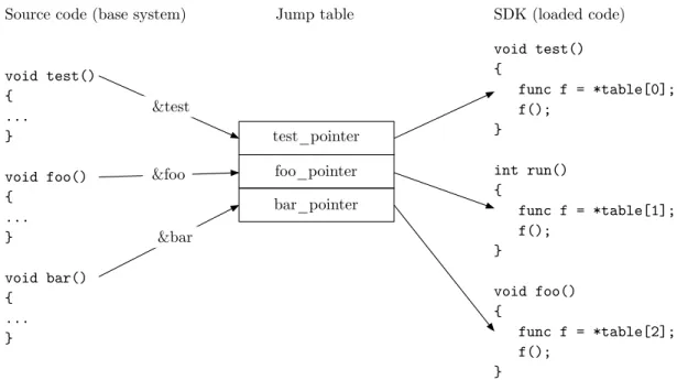
At the base of the interface connecting the loaded code is a jump table. As pictured in Figure 4.1, it is an array of function pointers by which loadable code can interact with the base system. Using this table, a Software Development Kit (SDK) can be created. This SDK comes with pre-defined headers and source files that abstracts the pointers in the jump table into regular functions and simplifies the development of loadable code.

void test() { ... } void foo() { ... } void bar() { ... } Jump table

Source code (base system) SDK (loaded code)

test_pointer void test() { func f = *table[0]; f(); } int run() { func f = *table[1]; f(); } void foo() { func f = *table[2]; f(); } foo_pointer bar_pointer &test &foo &bar

Figure 4.1: Showing how the jump table works (pseudo C code)

Figure 4.1 shows how the loaded code can interact with the base system, which defines a set of functions, via a jump table. It starts in the base system which contains a set of functions. A reference to the memory location for each of these functions are created and placed in an array. These references are what the loaded code uses to utilise functions that the base system provides, the array becomes a jump table since its content can be used to look up addresses to functions and then jump to them. When the loaded code is executed a reference to the jump table is passed to it and the loaded code gets access to

4.2 Solution

all function pointers inside of it. The SDK is then created by dereferencing the function pointers and wrapping them inside new functions (as seen to the right in Figure 4.1). This SDK can then be used to develop the loadable code without having knowledge about the jump table or any function pointers. The wrapper functions can be executed which in turn will execute functions inside the base system via the reference in the jump table.

4.2.3 Loadable Code

Code that will be loaded is created almost the same way as any regular C program, with a few exceptions. It needs to be linked in a specific way and it needs to implement a different starting point than the regular main() function. The application needs to do some setting up before the application actually can execute. It needs to set up the SDK and the jump table so functions in the base system can actually be called from the application. Therefore, the actual entry point is defined as start () which will then call main() at the end to execute the application. Starting with the main() function, this is purely an aesthetic choice and will give developers using the SDK, a feeling of total abstraction from the jump table, base system and hardware. It will be just like developing standard C-code using a library.

ARM GCC compiler is capable of creating something they call position independent code/executables. This produces executable code that does not depend on where it resides in the memory when it is accessing its data and functions. Position-dependent code has addresses, put into the binary code during linking, that defines where the processor should jump to continue execution. Code independent of it position instead has offsets, basically telling the processor to jump a certain amount of steps forward or backwards. This fea-ture of the linker allows us to compile code that can be fitted anywhere inside the memory where there is room for it.

4.2.4 Loading and Executing

The application is loaded as a byte stream. For the purposes of this study (and simplicity of development) it is enough to store it as a byte-array inside the base system. However, there is no limit to where it could be placed. It could be loaded from an external memory module or for example via Bluetooth. The base system then places this byte array in memory, both RAM and FLASH is possible1. In the developed prototype the binary is placed in RAM in order to get the largest, possible overhead by loading external code.

1

4. Implementation

Since our microcontroller is based on the Cortex-M3, which is of the Harvard architecture, RAM and FLASH are separated for increased performance. Therefore execution might become slower due to the limit of the buses, not just the overhead of jumping between application and firmware and the delay of loading it into memory.

When the application is placed in memory a pointer to the start of it is created and this pointer is what is going to enable the handing over of the execution to the loaded code. By creating a function from the pointer of the type void, taking a parameter of type unsigned integer, the entry point will look like: void start(unsigned int). When calling this function, e.g. passing a reference to the jump table, the execution of the loaded code is performed.

5

Experiment

5.1

Overview

The experiment conducted was testing prime numbers. The microcontroller applications created was testing various amounts of prime numbers and then the time needed to com-plete the tasks was compared. The algorithm used to test prime numbers was based on the fact about prime numbers known as 6k ± 1 which says that all prime numbers follow the form 6k±1. All integers can be represented by 6k+m where m ∈ {0, 1, 2, 3, 4, 5} and k ∈ Z (all integers). From this it can be concluded that if m ∈ {0, 2, 3, 4} the integer cannot be a prime number since 6k + 0 = 6 ∗ (1k + 0), 6k + 2 = 2 ∗ (3k + 1), 6k + 3 = 3 ∗ (2k + 1) and 6k + 4 = 2 ∗ (3k + 2). They are all divisible by denominators others than 1 or themselves making only m = 1 and m = 5 possible prime numbers. 6k + 5 = 6(k + 1) − 1 and therefore the final form for prime numbers can be written as 6k ± 1. Integers of the form 6k ± 1 are further examined to ensure that it is in fact only divisible by itself and 1. By elim-inating the integers not following the desired form the number of fully examined integers are reduced to one third of the total integers. Pseudocode describing the algorithm used is presented in Figure 5.1.

Two microcontroller applications was developed, one using the conventional method and one utilising the created prototype. The intention was to find out how much overhead there was when testing prime numbers, based on the algorithm in Figure 5.1, using a jump table in an application loaded during runtime.

Implementing this as a conventional microcontroller application is straightforward, the interesting part is the flow of the loaded code. What was done was implementing the next number and test functions in the base system and then have the loaded code call these via a jump table. In the conventional application it would all be implemented in the application code. Since every number tested had caused the execution to jump between the application and the base system two times, there was an overhead and how it affected the execution time could be measured.

5. Experiment let number = 0 next number() number = number + 1 return number is prime(n) if n <= 1 return false else if n <= 3 return true

else if n mod 2 == 0 or n mod 3 == 0 return false let i = 5 while i * i <= n if n mod i == 0 or n mod (i + 2) == 0 return false i = i + 6 return true

Figure 5.1: Pseudo code for determining if a number is a prime number

5.2 Equipment

The number function is basically a counter that returns the next number that should be tested every time it is called, this also allows us to prove that data can flow between the base system and the loaded code. The testing function takes an integer as a parameter and runs it through the algorithm in Figure 5.1 which returns whether it is a prime number or not.

5.2

Equipment

The experiment was performed with a STM32F103C8T6 microcontroller. It was mounted on a development board called the blue pill, available primarily from Chinese manufactur-ers via websites like eBay and othmanufactur-ers like it [26]. The microcontroller features a Cortex-M3 core. The core itself is based on the Harvard architecture which allowed developers at ARM to speed up execution speeds without increasing the clock speed of the processor [27]. The STM32F103C8T6 features 64Kb flash memory, 20Kb SRAM and a 72MHz processing unit [10]. It was chosen since it also includes built-in support for serial uploading of programs, enabling easy flashing via standard USB serial interface instead of a separate hardware programmer. High availability at retailers and hardware specifications low enough, to meet the requirements to be called low-end, made it a suitable test object for this experiment.

The experiment also included running on emulated hardware by using qemu. qemu is an open-source software capable of emulating a wide range of hardware. This allowed testing the developed system without uploading it to a physical microcontroller. The advantages offered are that qemu are able to print to the terminal, useful for debugging, and the ability to develop tests that will run autonomously and be timed with ease. The microcontroller used for this part was a STM32F103RBT6 circuit which has an almost identical 32-bit ARM Cortex-M3 core to the real hardware used [10]. Including qemu in the experiment is of interest since it is then possible to test how well execution times of the emulator relates to the actual hardware.

An Arduino device will also be used to measure execution time of the STM32F103C8T6 during the experiment. The reason for using an Arduino board for measuring is ease of programming and that the Arduino libraries already contain timekeeping functionality [28].

5. Experiment

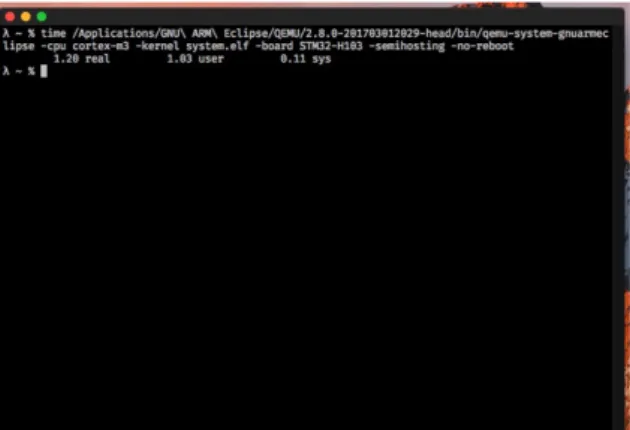
Figure 5.2: Screenshot of terminal emulator showing how the time utility measures execution time of a process.

5.3

Measurement

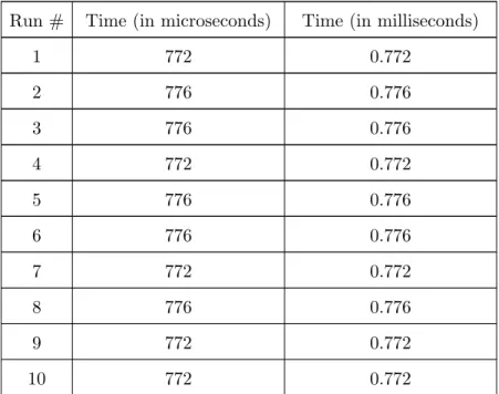
Measuring the execution times of the applications was essential to the study and unbiased, accurate measurement methods were needed. Different methods were used for the physical and emulated hardware. All tests were executed ten times and then the mean value was used to do the comparison.

5.3.1 Emulated Hardware

After the calculations were done semihosting, an interface for interactions between mi-crocontroller and debugger, was used to shut down the mimi-crocontroller. qemu supports the semihosting interface and upon receiving the command to shut down it will terminate itself. This can be used to measure the execution time using the Unix time command which will start the counter when the process starts and then stop it when the process terminates. After the process measured has stopped the execution time will be printed out in the terminal as seen in Figure 5.2.

5.3.2 Physical Hardware

Instead of using semihosting on the physical hardware a second microcontroller was used to measure the execution time. An Arduino board monitored a pin on the STM32F103C8T6 microcontroller. When the STM32 microcontroller started executing it set the pin to HIGH and when it finished the execution it set it to LOW. Meanwhile, the Arduino board was constantly checking the state of the pin. When it was set to HIGH the Arduino started to count and when it was set to low again it stopped the counting and printed the resulting time over a serial connection. The Arduino measures time in microseconds [28].

5.3 Measurement

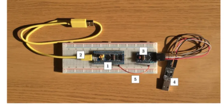
Figure 5.3: Image showing the setup with the STM32F103C8T6 development board and the Arduino board. 1. STM32F103C8T6 ARM Development board 2. USB cable supplying power to the ARM development board 3. Arduino board 4. USB to Serial converter, connecting the Arduino to a computer 5. Wire connecting the output pin on the ARM development board to the Arduino board.

This all resulted in very accurate and consistent measurements of the execution. How all the parts were connected can be seen in Figure 5.3.

6

Results

6.1

Execution times

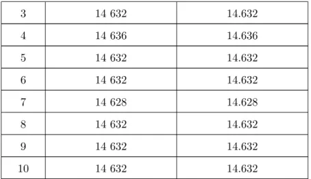
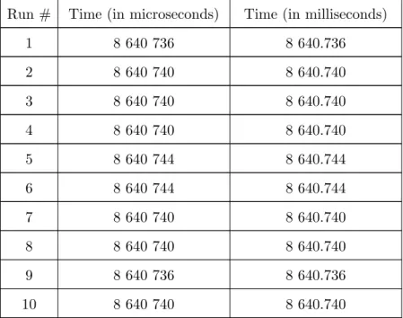
The data acquired from the experiment resulted in a set of mean times (presented in Table 6.1). These times can be used as an indication of the performance difference between the different ways of running applications on microcontrollers that we are testing. The times presented in this chapter are a summary of all the data and the mean times have been rounded to two decimal places for readability. The raw data has been placed in the appendix to this paper.

Number of primes Hardware (Traditional) Hardware (Loadable) Emulator (Traditional) Emulator (Loadable) 100 _(100%)0.57 _(135%)0.77 _(100%)1 136 _(101%)1 147 1 000 _(100%)12.45 _(118%)14.63 _(100%)1 152 _(100%)1 154 10 000 _(100%)300.82 327.25_{(109%) (100%)}1 187 _(105%)1 247 100 000 8 428.76_(100%) 8 640.74_{(103%) (100%)}1 959 _(131%)2 568 1 000 000 256 213.42_(100%) 258 739.47_{(101%) (100%)}16 909 23 660_(140%)

Table 6.1: Summary of all mean times calculated from the collected data, rounded to two decimal places. Times are in milliseconds.

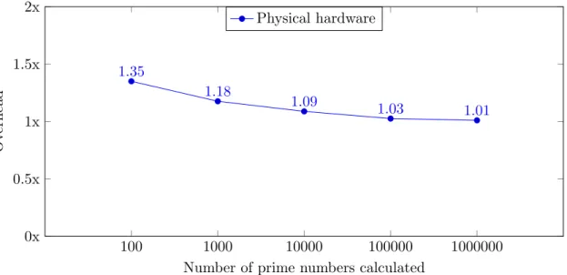
Figures 6.1 and 6.2 show how much the performance differs between running code the traditional way on microcontrollers and using the prototype created in this study. The difference is calculated by dividing the execution time of the prototype with the execution time of the conventional microcontroller application.

6.1 Execution times 100 1000 10000 100000 1000000 0x 0.5x 1x 1.5x 2x 1.35 1.18 1.09 _1.03 1.01

Number of prime numbers calculated

Ov

erhead

Physical hardware

Figure 6.1: Showing the difference in performance when calcu-lating primes, using different kinds of applications, on physical hardware. 100 1000 10000 100000 1000000 0x 0.5x 1x 1.5x 2x 1.01 1 1.05 1.31 1.4

Number of prime numbers calculated

Ov

erhead

Emulated hardware

Figure 6.2: Showing the difference in performance when calcu-lating primes, using different kinds of applications, on emulated hardware.

6. Results

Figure 6.1 shows a smooth curve. This is the resulting performance hit taken when running loadable code, as opposed to running traditional code. The calculations were performed on real hardware which means that the entirety of the processors resources were dedicated to them.

Figure 6.2, on the other hand, shows a reversed curve with more irregularities. It is the result of running the same tests, only on emulated hardware instead of real. Unlike when running on real hardware, this runs in a process among several others in an operating system.

6.2

Code Size

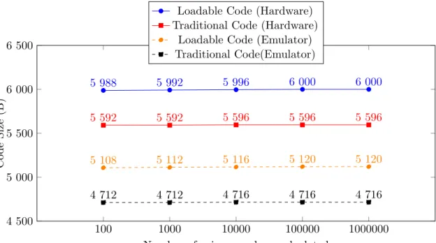
Figure 6.3 displays the sizes of all microcontroller applications tested. Sizes are displayed in bytes (8 bits). Applications enabled to load external code also has this code included in its total size since that code is essential to running the experiment successfully.

100 1000 10000 100000 1000000 4 500 5 000 5 500 6 000 6 500 5 988 5 992 5 996 6 000 6 000 5 592 5 592 5 596 5 596 5 596 5 108 5 112 5 116 5 120 5 120 4 712 4 712 4 716 4 716 4 716

Number of prime numbers calculated

Co

de

Size

(B)

Loadable Code (Hardware) Traditional Code (Hardware)

Loadable Code (Emulator) Traditional Code(Emulator)

Figure 6.3: Showing the difference in code size when calculating primes, using different kinds of applications, on both physical and emulated hardware. Sizes are shown in Bytes.

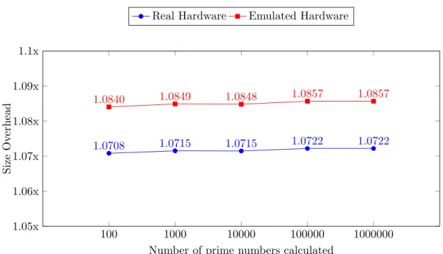
Figure 6.4 displays the size overhead for microcontroller applications running on both real and emulated hardware. The size of the applications with loadable code was divided with the size of the traditional microcontroller application.

6.2 Code Size 100 1000 10000 100000 1000000 1.05x 1.06x 1.07x 1.08x 1.09x 1.1x 1.0708 1.0715 1.0715 1.0722 1.0722 1.0840 1.0849 1.0848 1.0857 1.0857

Number of prime numbers calculated

Size

Ov

erh

e

ad

Real Hardware Emulated Hardware

Figure 6.4: Showing the overhead, in terms of code size, between traditional applications and applications with load-able code. Results for both physical and emulated hardware are included.

7

Discussion

7.1

Emulated Hardware

In order to discuss the results in the best possible manner the results from the emulated hardware should first be analysed. The attempt to measure execution times on emulated hardware was semi-successful at best. The microcontroller applications did run and the emulator was a very useful tool during the implementation stage of this study. Not having to reupload the code to a microcontroller on every change made the whole process a lot easier. It also provided several useful error messages if something went wrong (e.g. trying to access unavailable memory).

When it came to the experiment, however, and it was time to measure the execution time the emulator proved itself to be very irregular and unreliable. As can be seen, by the resulting execution times, the emulated results in no way follows the same pattern produced by the actual hardware. The emulating software never claimed to be accurate in its implementation but no research was found on this subject. Therefore, the interest in exploring whether the software would be useful when measuring execution times arose. The blame for irregularities can not only be placed on the emulator though. Not only does it not claim to be completely accurate but it also runs on top of an operating system. This means that the emulator process is controlled by the operating system and not fully capable of controlling how it executes. Depending on how the operating system decides to schedule other running processes (and starting new ones) the execution times of the emulator might be tampered with. Increasing the number of primes means longer execution times and more time for the operating system to interfere with how the emulated microcontroller executes the code.

Due to the irregularities and inaccuracy of the emulator the produced execution times from these experiments have been excluded from the discussion. Since they do not actually represent the reality there is no further point in comparing them to the measurements produced by the physical hardware.

7.2 Overhead

7.2

Overhead

The results provided by the physical hardware proved to be highly accurate and consistent. The execution times sometimes differ with a few microseconds which can be traced back to the Arduino board lacking the high resolution needed when counting microseconds.

7.2.1 Performance

The resulting execution times show an overhead when running loaded code, as expected. When just calculating 100 prime numbers there is actually a significant overhead of 35%. However, the overhead decreases as the number of calculations increases. When calculating 100 000 prime numbers it is 3% and when calculating 1 000 000 prime numbers the overhead goes down to just 1%. The 1 000 000th prime number is 15 485 863 which is the amount of numbers that has to be checked before reaching 1 000 000 found prime numbers. Considering that checking each number requires two functions to be called via the jump table, this means that in total 30 971 726 jumps are made from the loaded code, via the jump table, to the base system and then back again. Doing this with an overhead of 1% (and decreasing) makes loadable code an interesting alternative to conventional microcontroller applications. 1% overhead meant about 2.5 milliseconds slower execution in the case of finding the 1 000 000 first prime numbers.

The decrease in overhead is most likely due to the loading of the code. The time measure-ments of the loadable code included both the loading and execution of the code, compared to the conventional applications that only measured the execution time of the application. Therefore, the total overhead of loaded code is the loading of the code and the slightly slower execution. When performing few calculations the time it takes to load the code is a lot longer in comparison to the execution time, resulting in a larger overhead. However, when many calculations are performed the execution time increases and the overhead created by the loading time decreases. As the execution time increases to many times the loading time the overhead created by loading code is decreased to an insignificant overhead. At 1 000 000 found prime numbers the total overhead is 1% and most of that is execution time. This is based on the fact that when calculating 100 primes the time difference is 20 milliseconds and when calculating 1 000 000 primes it is over 2 500 milli-seconds, both cases involves loading about the same amount of code. Based on this it can be deduced that the overhead from loading code is less than 20 milliseconds in all tests and this overhead is less when calculating 1 000 000 primes than 100 primes.

7. Discussion

7.2.2 Code Size

While the objective was to use the storage more efficiently, it was assumed that there was going to be an overhead in size when compared to conventional applications. This overhead was to be created by incorporating code that made it possible to load and unload code on demand. This added functionality, while increasing the total code size, can be considered to compensate for the larger applications since it is then possible to store more code outside of the microcontroller.

The results indicate a very small overhead (about 400 bytes) in order to enable load-able code. For the example used in the experiment this meant less than 1% overhead. Given that the system enables the loading of huge amounts of code it is a very reasonable overhead. In the chapter about related work alternatives were discussed, such as virtual machines and interpreters. Most of these require several kilobytes of memory which in-dicates that the overhead of the prototyped system fits at least twice inside any of these other solutions (Tapper excluded which could become as small as 230 bytes).

There was also some minor changes in code size depending on how many prime numbers was attempted to be found. The applications grew a few bytes when the amounts of prime numbers increased. A reasonable explanation could be that the compiler could optimize the code better when smaller amounts of prime numbers are calculated. The compiler probably optimises some variables and represents them with a smaller data type and thereby saving some bytes in the process.

7.3

Considerations

7.3.1 Application Development

The system implemented enables developers to write microcontroller applications without having any knowledge about the hardware. The base system can abstract the hardware in the functions stored in the jump table which can be called by developers, through a SDK, who do not have to care which pin a LED light is connected to. Since code can be loaded from an external source application developers do not need to learn or understand how the uploading via a programmer works. They can, for example, just transfer the finished code to a SD card. The abstraction of the hardware also open up for cross-platform applications. All the application code needs to do is call a function, via the jump table, and then the base system can implement the hardware specific logic.

7.3 Considerations

7.3.2 Security

As mentioned in the background theory, dynamic linking enables code to be linked first when it is to be executed. It blindly accepts any code that fits into the hole created by the linker. The loadable code compiled for the prototype, from this study, works the same way. It accepts an address to a jump table when it is first executed and then it uses the table for every external method call without any verification. This enables code pieces to be patched individually, which is a good thing, but it also enables maleficent attacks. Since the loaded code can not differentiate flashing a led light and getting stuck in an endless loop there exists an opportunity for harmful code to be injected. In a closed system this is not an issue but if code was to be received through wireless communication channels the system is vulnerable. The data received has to be verified before it is executed in order to ensure that the correct code has been received.

7.3.3 Reliability

Having dynamic parts in a system can make it more prone to failures. If an application expects an integer as input but receives a string it might fail if there is no error handling implemented. The same goes with loadable code. Microcontrollers are very useful since they have their code burnt into the memory circuits and always executes it the same way. Introducing loadable code also introduces some weaknesses to the system that has to be taken into consideration. There has to be memory available to, temporarily, store the code. If something else is taking up all memory the system will fail the loading. The idea of loadable code was to split a large system into tiny pieces of code that each can perform a single task. This would allow a total size of code that is larger than the storage memory on the microcontroller, but there still need to be memory available for a small piece of code.

Reading the byte array representing the code might fail. A corrupted SD card or a bluetooth transfer that looses its connection introduces exceptions that the system must be able to handle in order to not crash. As with the security aspect of the system this is another reason to verify the code before loading it. Verification causes additional overhead but in some cases it might be required.

8

Summary

8.1

Conclusion

The research questions in this study was: ”What kind of overhead follows with a more storage efficient system? Is this system a viable alternative to the traditional way of run-ning code?” (RQ1) and ”How can a system be implemented, on low-end microcontrollers in native code, that uses storage more efficiently?” (RQ2). To answer RQ2 a system was hypothesised and then implemented using a jump table. This jump table enabled code loaded at runtime to execute functions located outside of itself. By being able to replace entire functions with a single function call the size of the loadable code was decreased. The fact that it is loadable enables storage outside of the microcontroller which would lead it to only occupy storage memory inside the microcontroller when it is executing.

To answer RQ1 the system designed was tested in a controlled experiment. From the results gathered it could be deduced that the execution time overhead could become as little as 1% and still be decreasing. The memory usage overhead turned out to be stable around 8.5% or 400 bytes. Considering these results it is safe to say that the overhead is very small as long as the number of computations performed by the applications is high.

However, this only answers the first part of the question. The second part (whether the system is a viable alternative to conventional applications or not) is not as easy to answer. More variables than just the overhead go into this. In the discussion chapter several considerations are brought up. All these come into play when answering whether the system is an alternate or not and there is still no definitive answer. It all depends on the purpose for which the system is developed for. Development requiring high reliability or security of the system might not benefit from a system that loads code during runtime. However, for casual purposes there is often no need to have complete security or reliability. By enabling the usage of cheaper microcontrollers, with low storage memory, in products, cheaper products can be produced. This could enable more people to be introduced to electronics otherwise unavailable to them. Learning to develop for microcontrollers also