Benefits of increased axle loads : method of calculation and its application to Swedish conditions

(1)

S TAT E NS Y A G I N S T I T U T • S T O C K H O L M

The National Road Research Institute, Stockholm, Sweden

BENEFITS OF INCREASED

AXLE LOADS

Method of Calculation and its Application to Swedish Conditions

by

Carl Erik Brinck

Proceedings

94

(2)

(3)

BENEFITS OF INCREASED

AXLE LOADS

Method of Calculation and its Application to Swedish Conditions

by

(4)

Lagerblads

AB RAGNAR LAGERBLADS BOKTRYCKERI KARLSHAMN 1968

(5)

Preface

In many countries, the roads being built today are designed for heavier axle loads than those permitted earlier. In several of the countries where the current limit is 10 (metric) tons an increase to 13 tons is being considered. In Sweden, too, an increase of the permissible axle load to 13 tons has been discussed in recent years.

A general increase in permissible axle loads would, however, require a vast amount of capital expenditure. At present, successive improvements of the bearing capacity of the road network in this country are taking place in order to permit a general increase of the permissible axle load to 10 tons. These improvements will in themselves, according to the estimates prepared by the State road authorities, cost about 6 billion Swedish kronor. (1 billion = 1,000 millions.)

A question that naturally arises in this connection concerns the economic benefits likely to result from such an investment. Hitherto, however, it has not been possible to find an answer to this question. This depends on a lack of statistical data and difficulties in using the data available and dealing systematically with all the factors which must be taken into account in a profitability analysis.

In the thesis presented here, a method of calculating the benefits of increased axle loads is described. The method is applied to Swedish conditions, and much effort has been made to ensure that the assumptions on which the calculation is based reflect the conditions which prevail in this country.

The work has been carried out at the National Swedish Road Research Institute, where I am employed to study road problems in general and road transport eco nomy in particular.

It is my sincere hope that this report will contribute to a better understanding of the intricate problem of the economic benefits of increased axle loads.

Finally, I wish to express my thanks to Mr. Nils G. Bruzelius, Head of the National Swedish Road Research Institute, whose keen interest in the subject with which I have dealt and whose advice and suggestions relating to this study and its publication have afforded stimulation and encouragement to me in my work.

I am also greatly indebted to Professor Sten Hallberg, Head of the Division of Highway Engineering at the Royal Institute of Technology, Stockholm, and member of the Board of the National Swedish Road Research Institute. I am indebted to him for his critical perusal of the manuscript.

(8)

Dr. Bertil Hållsten of the Stockholm School of Economics, who has read the manuscript and made many valuable comments,

Dr. Torbjörn Thedéen of the Division of Mathematics, the Royal Institute of Technology, Stockholm, for valuable advice and discussion,

and my colleague at the National Swedish Road Research Institute, Mr. Björn Örbom, wlio has studied chapter 2 and made many valuable suggestions.

In addition, I express my thanks to my translator, Mr. David Knight, and to Mr. Manfred Bode of the Institute of Reactor Research at the Royal Institute of Technology, Stockholm, who has checked my calculations.

Stockholm, May 1968 Carl Erik Brinck

(9)

CHAPTER 1

Introduction

During the last 15 years the axle load permitted on Sweden’s most densely fre quented highways has been increased from 7 to 10 tons1.

This increase in the permissible axle loads has been decided by the road authorities as a consequence of the general development in the transport sector. A distinctive feature of this development over a sequence of years has been a successive change in the make-up of the truck stock towards an ever-increasing number of bigger load carriers which, with regard to engine power and other design features, allow for heavier maximum payloads than can be permitted on all highways with the current axle load limits.

The industrial and commercial community regards a switch to bigger load- carrying units as a vital ingredient in its efforts to improve transport economy and is therefore making demands for an improved standard of bearing capacity on the road network and for higher axle load limits.

During recent years the road authorities have made improvements to a great many highways in the Swedish road network in order to reduce transport costs and therefore conduce to industrial growth and competitiveness. The National Swedish Road Administration has pointed out on numerous occasions that one of the primary objectives of road investments is to provide highways with a bearing capacity good enough to meet the requirements of freight transport, thereby making it possible to cut down transport costs (l).2

It is only natural that the highway construction policy is judged by industry according to the effect it has on company costs and competitiveness. It is highly probable that the use of big load-carrying units would result in substantial eco nomic benefits for companies with heavy transport costs. Such companies have therefore benefited financially from those increases already made in the legal axle loads, but they would undoubtedly welcome all further improvement of their trans port economy. This desire is clearly expressed in articles and lectures by represen tatives of the industrial sector, who point to the ever-increasing growth in road haulage as a motive for further highway improvements which would allow the use of even bigger vehicles.

1 Tons in this paper = metric tons 2200 lb). 2 Numbers in brackets ( ) refer to “ References”.

(10)

Freight transport by trucks expressed in billion ton-km is increasing at a far more rapid pace than the total amount of freight transport in Sweden. According to Godlund (2), this total amount has practically doubled from 1950 to 1964, whereas the share carried by trucks has undergone an almost fourfold increase during the same period. This development in itself is by no means surprising, since road haulage offers considerable advantages with regard to speed, convenience, etc. There is, however, no doubt that the increases in axle loads so far introduced have made it possible to use big and therefore economical truck-trailer combinations. Thanks to this, it may safely be assumed that the increased axle loads have con tributed effectively to the expansion in the trucking sector. The greater this expansion, the more justification there has been for referring to its extent and to its importance for the whole transport sector as a strong motive for further in creases in the legal axle loads. In the long run this reasoning will probably result in higher axle loads than those permitted today and thus in a still further increase in the extent of road-haulage traffic. Bearing this in mind, one may well ask by how much the permissible axle load will be increased next time and on what grounds this decision will be taken.

A higher axle load necessitates a highway construction of greater bearing capacity than a lower one. As a rule, the bearing capacity can be improved by increasing the thickness of the pavement, but this in turn involves higher pavement costs. The road authorities have been fully aware that higher axle loads mean more expensive highway construction. It has, however, been difficult to calculate the amount of such additional expenditure and to weigh this in a methodical manner against its usefulness to the industrial sector and against the benefits of other capital-consuming measures. Such measures may in themselves be urgent but many of them are difficult to evaluate in monetary terms, such as measures resulting in time savings for the highway users or promotion of road safety.

Attempts to compare the economic benefits of an increase in permissible axle loads with the expenditure involved have nevertheless been made. In the chapter of the 1958 Road Plan (3) which is concerned with the standard of bearing capa city, it is reported that the incremental costs for higher single-axle and tandem- axle loads are of such magnitude that they can scarcely be counterbalanced by the benefits in lower transport costs resulting from the insertion of heavier vehicles. This assertion indicates that an increased legal axle load would not be a paying proposition in the light of the incremental highway costs. It is not clear what is meant by »scarcely» in this context, nor are any calculations presented.

This quoted statement, however, has evidently not been accepted as a guiding principle by the road authorities, since the permissible axle load has actually been increased since 1958 on those highways which form the so-called heavy road network. In the Road Plan, mentioned above it is also pointed out that if the legal axle load is to be increased, a uniform standard for the entire road network should

(11)

be aspired to. This implies that all highways must be designed for the same axle load despite the great discrepancies in the freight tonnages carried on different parts of the network. This opinion is also untraceable in the most recently ratified axle load increase, which on the contrary provides an example of a contradictory opinion, involving differentiation of the bearing capacity in view of the varying extent of road-haulage traffic on different highways. According to an opinion stated in »Optimum Axle Loads» (4), the quantity of freight carried is a factor of vital importance to the axle load which may be regarded as optimal for the highway concerned. As this quantity of freight grows, the demands for increased legal axle loads appear to be more and more justified.

As regards the heavy road network in Sweden, the National Road Adminis tration has also asserted that an increase of the legal axle load to 10 tons should be carried out initially on those heavily frequented highways which form long, continuous transport routes. This probably means that the urgency of an axle-load increase should be judged in view of the importance of the highways concerned as a road-haulage route, i.e. according to the tonnage of freight transported. From this it may be concluded that the tonnage moved is regarded by the authorities as the most suitable basis of judgement when considering a future increase in the legal axle load.

This basis of judgement, however, is not sufficient. The primary consideration must be whether and on what conditions an increased axle load is economically justifiable from the standpoints of both vehicle-operating costs and highway costs. All the funds allocated to the highway system are obtained through special taxes. The portion of such taxes which is collected from road-haulage trucks is allowed for in the transport tariffs and is reflected in commodity prices to a corresponding extent. These taxes are thus actually paid by the consumers, who are therefore naturally interested in keeping transport costs at as low a level as possible. It devolves upon the road authorities to decide how great a share of the available funds should be invested in improved bearing capacity, with due consideration to transport economy. A decision of this kind could be based on or facilitated by a profitability analysis in which the estimated cost decrease on the transport side is regarded as interest or profit on the capital invested in the road network.

In any such analysis, the yield in the form of reduced vehicle-operating costs must be considered in the light of the total tonnage moved on the highway to which the analysis refers and not merely to the savings which can be achieved for effectively utilized individual vehicles. Furthermore, the result of any such analysis will depend on the number of vehicles which may actually be expected to take advantage of the higher axle load. This figure must, therefore, also be determined.

This provides the prerequisites for an integral view of the complex axle-load problem, where the question of an increase can be judged with due regard to the

(12)

increment in highway costs, the decrement in vehicle-operating costs and the quantity of freight carried, and where the anticipated profit on the vehicle-operating side and the calculated expenditure on highway construction can be compared with each other. Up to now, such a comparison has been lacking, both with regard to the data on which an analysis of this kind should be based and with regard to the method of calculation which should be used. In consequence, less attention has been paid to highway costs and actual tonnages moved than to the savings in vehicle-operating costs, and this in turn has led to a lack of balance in the basis on which decisions are made. According to generally recognized profitability prin ciples, the anticipated profit on a project should give sufficient return on the in vested capital if the project is to be realized. These same principles should also be applicable to investments in the road network.

A manner in which a calculation of this kind can be prepared will be described in this study and applied to those cost figures which are currently available on highway construction costs and vehicle-operating costs. The figures on freight tonnages and on the distribution of freight on the Swedish highways which are available or can be estimated will also be taken into consideration.

In this first chapter a brief introduction has been given. The following study is presented in chapters 2— 6.

Chapter 2 deals with calculation of highway costs based on Swedish conditions. The highway costs will be studied on the assumption that the axle load is varied in three stages from 8 to 14 tons. Firstly, a highway is designed for a single-axle load of 10 tons and a cost estimate for this highway is prepared. After this, on otherwise unaltered conditions, the axle load is assumed to be 8, 12 and 14 tons, thereby enabling the incremental highway cost for each axle-load level to be determined.

Chapter 3 is concerned with calculation of vehicle-operating costs under the same conditions. In a similar manner, the differences in vehicle-operating costs arising out of the assumed axle load increases from 8/12 to 10/16, from 10/16 to 12/20 and from 12/20 to 14/241 tons are determined. As will be seen from the axle loads mentioned, the calculations in chapters 2 and 3 take into account axle loads for which currently existing highways and vehicles are not designed and for which the costs are therefore unknown. In these cases, the calculations must be based on the experience gained from known highway costs and vehicle types.

1 These combinations are chosen due to the practice in Sweden and other countries as regards the legal limits for single- and tandem-axle loads. They do not, however, exactly reflect the equivalence between single and tandem axles as far as the load on a pavement is concerned. The term 8 /1 2 , 10/16 etc. as used in this study is a compound expression, in which the first component refers to a single axle, and the second one to a tandem axle.

(13)

In chapter 4, an account is given of a profitability analysis, and an application to the specific results from chapters 2 and 3 is presented.

Chapter 5 deals with the distribution of the freight tonnage carried on the Swedish highway network in 1965 and the ton-km data.

In chapter 6, finally, an account is given of the conclusions arrived at from specific results in chapters 4 and 5.

(14)

CHAPTER 2

Highway Costs

2.1 Average Cost of Pavement Construction

The highway cost can in this context be confined to the cost of pavement con struction, since in principle only the pavement thickness changes with the magni tude of the axle loads. The greater bearing capacity necessitated by a higher axle load in comparison with a lower one is generally obtained by an increase in the pavement thickness.

The cost of this increased thickness constitutes the incremental cost necessitated by the higher axle load.

The thickness and the construction cost of the pavement can vary from one highway project to another, even though the highways concerned are designed for the same axle loads, and have the same road width and the same standard other wise. The variations in thickness are due mainly to differences in the properties of the foundation soil. A thicker pavement will be required on a weak foundation soil than on a soil of higher bearing capacity. Variations in construction costs are due partly to differences in pavement thickness and partly to normal price fluctua tions.

Because of these variations, it is necessary to calculate the cost of a pavement which can be regarded as a representative average for Swedish conditions.

A calculation of this kind has been made at the National Swedish Road Admini stration (in the following referred to as the Road Administration) on the basis of the cost accounts in 156 approved work plans for highway projects in different parts of Sweden during the period 1961— 1965. The costs referred to in the following have been converted1 to the 1965 monetary value.

The calculations have been made for three highway sections with widths of 6.5, 9 and 13 metres respectively. The sections are divided into carriageway and shoulders. In the 6.5-metre section, the carriageway is 6 metres wide and each shoulder 0.25 metre wide. In the 9-metre section, the carriageway is 7 metres wide and each shoulder 1 metre. In the 13-metre section, the width of the carriageway is 7 metres and that of each shoulder 3 metres.

1 According to the road construction index, prepared by The Associated General Contractors and House Builders of Sweden.

(15)

For the 6.5-metre section, the cost per metre highway has been determined on the basis of 40 work plans from all parts of the country, although the majority, 29, of these refers to the northern part of Sweden. The 9-metre section has been processed on the basis of 62 work plans, of which one third refers to highway pro jects in the central and northern counties of Sweden, while the southern counties account for the remaining two thirds. The 13-metre section, finally, is based on 54 projects, barely half of these in southern and central Sweden.

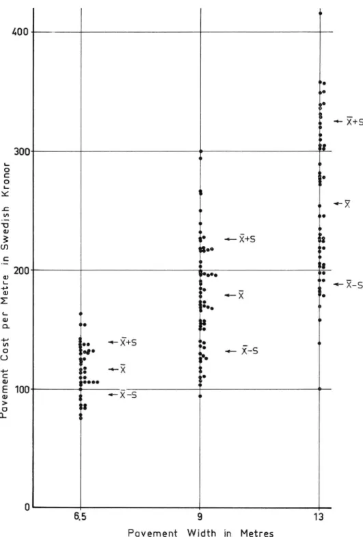
The road length in the studied projects varies from 1 to 30 km. The total road length of all the highway projects studied amounts to 1,104 km (389 for the 6.5-metre section, 378 for the 9-metre section and 337 for the 13-metre section). The results of these studies are illustrated diagrammatically in fig. 2.1. Each dot indicates the average cost in kronor per metre for each project. The arithmetic mean and standard deviation have been calculated for each highway section.

As may be seen from fig. 2.1, the dotted values show great variations. This is only natural in view of the different conditions which may have been encountered in the various projects with regard to the bearing capacity of the bed material itself, the distance to gravel pits, etc. If the standard deviation (and the coefficient of variation) is calculated for the individual values, the results given in table 2.1 will be obtained. (The reported variations will be discussed in chapter 6.)

Table 2.1. Average pavement costs for 156 highway projects.

Highway Section

Pavement Cost kronor per metre

Standard Deviation kronor per metre

Coefficient of Variation % 6.5 117 22 19 9 179 47 26 13 256 68 26

In view of the comparatively extensive material studied and of the relatively even distribution of the highway projects throughout the country, it may be assumed that the influence of different types of foundation soils and local price fluctuations has been largely evened out. The average figures listed in table 2.1 may therefore be considered to be representative for the average cost of pavement construction for Swedish conditions in the 1965 monetary value, including subbase course, base course and bituminous surfacing.

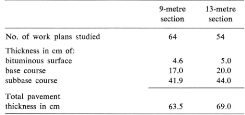
For the 9-metre and 13-metre sections, the calculation results are reported in greater detail than for the 6.5-metre section, and both average total pavement thickness and thickness and price per metre for each course are stated. This provides a means for estimating the average bearing capacity, which will be de scribed further on. This detailed account is presented in table 2.2.

(16)

Fig. 2.1. Pavement cost per metre for 156 highway projects, (x and s stand for estimated arithmetic mean value and standard deviation respectively.)

(17)

Table 2.2. Thickness of the different courses in the 9-metre and 13-metre sections.

9-metre section

13-metre section

No. of work plans studied 64 54

Thickness in cm of: bituminous surface 4.6 5.0 base course 17.0 20.0 subbase course 41.9 44.0 Total pavement thickness in cm 63.5 69.0

2.2 Bearing Capacity of the Studied Sections

According to the Swedish design regulations, pavements must be designed for a single-axle load of 10 tons. In addition, allowance must be made for the volume of traffic according to one of the following two alternatives:

1. Number of freight vehicles per day during the thawing period. 2. Average daily traffic during June, July and August (Summer-ADT).

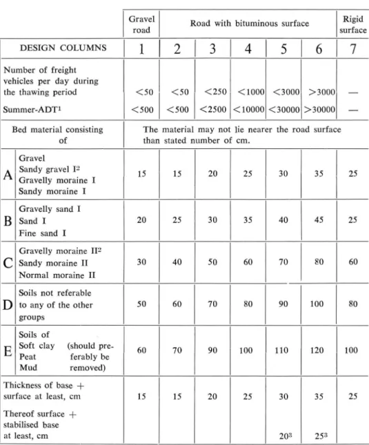
The regulations are reproduced in tabular form in “Directions for Highway Construction” (5) (in Swedish). The table is so arranged that the pavement thick ness can be found if the nature of the roadbed (material groups A— E) and the magnitude of the traffic volume (columns 2— 6, gravel roads excepted) are known. This table is shown here as table 2.3.

The figures quoted in the table are considered by the Road Administration to correspond to a designed single-axle load of 10 tons. However, no indication is given of how many load applications with an axle load of 10 tons they are intended to represent. For this reason, the figures on traffic volume given at the top of the table do not provide a true measure of the actual traffic load (axle load and number of load applications). A question of great interest here is: “For what traffic load are the pavements included in table 2.1 actually designed, i.e. what bearing capacity corresponds to the costs indicated in table 2.1?”

The pavement thicknesses are specified in table 2.2, from which it is seen that both the thickness of each course and the sum of the courses, i.e. the total pavement thickness, are specified for the 9-m and 13-m sections. The pavement thickness of the sections can be used together with column 41 in table 2.3 to determine the soil types which correspond to these pavement thicknesses. As may be seen from table 2.3, the thicknesses given in table 2.2, i.e. 63.5 and 69 cm, correspond to material group C and to the border between C and D respectively.

(18)

Table 2.3. The Swedish Road Administration’s Design Table. This table is translated from (5)

Gravel

road Road with bituminous surface

Rigid surface

D ESIGN COLUMNS

₁

₂

₃

₄

₅

₆

₇

Number of freight vehicles per day during the thawing period Summer-ADT1 < 5 0 < 5 0 0 < 5 0 < 5 0 0 < 2 5 0 < 2 5 0 0 < 1 0 0 0 < 1 0 0 0 0 < 3 0 0 0 < 3 0 0 0 0 > 3 0 0 0 > 3 0 0 0 0 —

Bed material consisting of

The material may not lie nearer the road surface than stated number of cm.

A

Gravel Sandy gravel I2 Gravelly moraine I Sandy moraine I 15 15 20 25 30 35 25

B

Gravelly sand I Sand I Fine sand I 20 25 30 35 40 45 25

C

Gravelly moraine II2 Sandy moraine II Normal moraine II

30 40 50 60 70 80 60

D

Soils not referable to any of the other groups

50 60 70 80 90 100 80

E

Soils of

Soft clay (should pre- Peat ferably be Mud removed) 60 70 90 100 110 120 100 Thickness o f base + surface at least, cm Thereof surface - f stabilised base at least, cm 15 15 20 25 30 203 35 253 25

1 Summer-ADT = average daily traffic during June, July and August. 2 I indicates frost-insusceptible and II frost-susceptible soils.

3 For base and subbase of broken rock or crushed stone, the thicknesses can be reduced by approx. 10 cm.

(19)

If a California Bearing Ratio (CBR) of 10, which according to an investigation by Bruzelius (6) can be regarded as corresponding to material group C, is taken as the starting point, the bearing capacity corresponding to the pavement thick nesses can be calculated. This is done with the aid of a design nomograph, which has been drawn up in a report published by the Highway Research Board (7). This nomograph is based on results from the AASHO Road Test, but is modified in that it can be utilized also for other road bed materials than that found on the test site and which was equivalent to a CBR-value of 3. It can, therefore, be applied in the present case, where the CBR-value is assumed to be 10.

Further, the value of the thickness index D from the test results has been modified in view of the fact that the AASHO Road Test was conducted for a considerably shorter period than corresponds to the normal service life of high ways. The values of D derived from the nomograph will therefore be greater than those reported from the test. They are designated Structural numbers instead of thickness index and are denoted D t instead of D.

The nomograph is reproduced in fig. 2.2.

Fig. 2.2.

Nomograph for highway pavement de sign. The scale on the left is an ex pression of the total load during the service life of the highway, the middle scale indicates the soil support (CBR) and the scale on the right affords a measure of the pavement thickness in inches.

The nomograph is reproduced from a report published by the Highway Rese arch Board (7).

(20)

The coefficients ai and a3 are assumed to have the same values as in the AASHO Road Test, while a2 is assumed to be 0.13 instead of 0.14. The figure 0.14 is valid for a base course of macadam. This type of base course is unusual in Sweden, where as a rule a crushed material — base gravel — is used instead. According to the report published by the Highway Research Board (7) mentioned above, the figure 0.13 is better than 0.14 for a material of this kind.

The coefficients, then, are given the following values: ai = 0.44 (corresponding to a bituminous surface) a2 = 0.13 (corresponding to base gravel)

a3 = 0.11 (corresponding to subbase sand)

As may be seen from table 2.2, no pavement thickness is given for the 6.5-metre section. The calculations described in the following therefore embrace the 9-metre and 13-metre sections only.

The 9-metre section

For the 9-metre section, the following value of D t is obtained:

D = (0.44 X 4.6 + 0.13 X 17 + 0.11 X 4 1 . 9 ) - ! - = 3.5

1 2.54

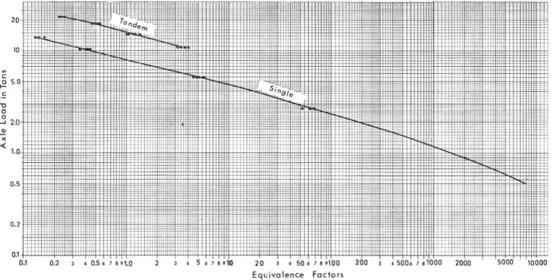
With Dt = 3 .5 and CBR = 1 0 , the number of axle applications with an axle load of 8 tons1 can be found from the lefthand scale in fig, 2.2, which gives a reading of 1.6 million axle applications. This is the same as about 0.7 million app lications with an axle load of 10 tons, which can be calculated with the aid of the chart in fig, 2.3. This chart is reproduced from “ Optimum Axle Loads” (4). It shows the equivalence factors of different axle loads according to the results from the AASHO Road Test.

This chart can be used to convert different axle loads into an equivalent number of 8-ton axle applications. The equivalence factor for 8 tons is 1.00. From the chart it is found, for example, that the equivalence factor for 10 tons is 0.44 and that for 4 tons it is 17, i.e. one application of an 8-ton axle load has the same effect on the highway as 0.44 applications of a 10-ton axle load or 17 applications of a 4-ton axle load. The stated equivalence factors are the mean values for the various test sections included in the AASHO Road Test.

1 Actually 8.2 tons (18,000 lb). 18

(21)

(22)

The 13-metre section

As shown in table 2.2, the pavement thickness is 5.5 cm higher for the 13-metre section than for the 9-metre section. Since both sections are designed in accordance with the same design table, the difference in thickness must be attributed to an average roadbed material that is weaker in the 13-metre section than in the 9-metre section. As pointed out earlier, this can also be found in the design table, where the pavement thickness for the 13-metre section corresponds to a material group on the borderline between group C and group D. The CBR-value for group C may be considered to be 10. Material group D corresponds to the roadbed material used in the AASHO Road Test, and this material had a CBR of 3. For the 13-metre section, therefore, the CBR should be less than 10 but greater than 3. If the CBR- value is assumed to be 7, we find:

Dt = (0.44 X 5 + 0.13 X 20 + 0.11 X 44)— *—= 3.8

1 2.54

According to the nomograph, this gives 1.8 million axle applications with an axle load of 8 tons or 0.8 million applications with 10 tons, i.e. roughly the same values as were found for the 9-metre section.

According to these calculations, both sections thus can withstand roughly the same load. As stated earlier, this is only to be expected, since they are both de signed in accordance with the same standards.

It might therefore be assumed that the pavements arc designed for a load of 0.8 million applications with an axle load of 10 tons. This value, however, will depend on the assumed value of the CBR. The measurements of the soil support (CBR-values) on different Swedish soils show substantial variations. In the in vestigation by Bruzelius (6), the CBR for sandy moraine is reported to be 9 and for clayey moraine 32. These figures are valid for saturated soil specimens. Both of these soil types are included in material group C or D.

It is, however, difficult to saturate specimens of soil with a high content of clay, e.g. clayey silt moraine, and for this reason laboratory tests on such soils may give higher figures than those actually corresponding to the supporting power of the soil in the natural state. The figure 32 can therefore be considered to be more unreli able than the figure 9. The assumed CBR of 10 for material group C shows good agreement with CBR-values determined in the U.S.A. (7), where the figure 10 is reported for soil type A-3, which according to the Highway Research Board classification is closely equivalent to the Swedish group C.

A CBR-value of 10 for group C is thus a plausible figure, but naturally it may also be both lower and higher.

As a rough estimate, however, it can be safely assumed that the pavements studied here are capable of withstanding a traffic load corresponding to approxi

(23)

mately 1 million applications with an axle load of 10 tons. After the pavements have been subjected to this traffic load, the quality of the highway may be assumed to have fallen to the level indicated according to the AASHO Road Test by a Present Serviceability Index (PSI) of 2.5.

2.3 Service Life of the Studied Sections

A question that is now of interest concerns how long a time it will take until 1 million applications by 10-ton axles have been reached, with due regard to the actual traffic load on a certain section of the road network.

The true traffic load can be determined with the aid of the vehicle loadometer (weight) studies conducted by the Road Administration (8) and the relationships between the equivalence factors of different axle loads shown in fig. 2.3.

At the 90 weighing points run by the Road Administration, loadometer studies were conducted in 1965 on a total of 1,216,516 vehicle axles, equivalent to

438,110 vehicles with an axle load of at least 1.25 tons. The results from these

studies can be split up among the following road categories:

E = National main roads included in the European arterial highway system

R = National main roads

L p = Primary regional roads L s = Secondary regional roads

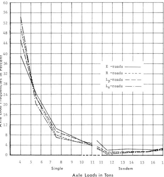
If the recorded axle loads within each of these four road categories (E, R, L p and L s ) are divided into the following classes

< 5 5— 6 7— 8 9— 10 > 1 0 tons (single axles)

and < 1 1 11— 12 13— 14 15— 16 > 1 6 tons (tandem axles)

the group of curves shown in fig. 2.4, can be plotted. Each curve represents the average for each individual road category. The material on which the curves are based is indicated in Appendix 1.

In 1965, about 10 % of the Swedish road network was open to 10/16-ton axle loads (10 tons for single axles and 16 tons for tandem axles). The highways in cluded in this heavy road network were almost exclusively roads of categories E and R. On other roads, the permissible axle load was 8/12 tons or less. However, as may be seen from fig. 2.4, the four curves run very close to one another. The proportion of axle loads of 10 tons or more for single axles and of 16 tons or more for tandem axles is practically the same for all the different road categories. The results of the loadometer studies do not show that the permitted axle load is different on different roads. It is, instead, made clear that the heaviest axle loads

(24)

Fig. 2.4. Number of weighed axles split up among different axle-load groups.

are distributed fairly evenly among the different road categories regardless of the axle load permitted on them. This is particularly true of axle loads of 10/16 tons or more, the proportion of which is at least as great on roads of category L s as on roads of categories E and R.

With the guidance of the results from the AASHO Road Test, the influence of different axle loads in respect of traffic load can be converted to an equivalent number of axle loads of a certain size, e.g. 8 tons. As explained earlier, this con version can be made with the aid of the diagram in fig. 2.3.

(25)

Using this diagram, it is now possible to determine the equivalence factors which correspond to the midpoint within the groups listed above. For the smallest and biggest axle loads, the “ group midpoint” must be estimated. For the lowest group, the figures 4 tons for single axles and 10 tons for tandem axles have been adopted, the corresponding figures for the highest group being 11 and 17 tons respectively.

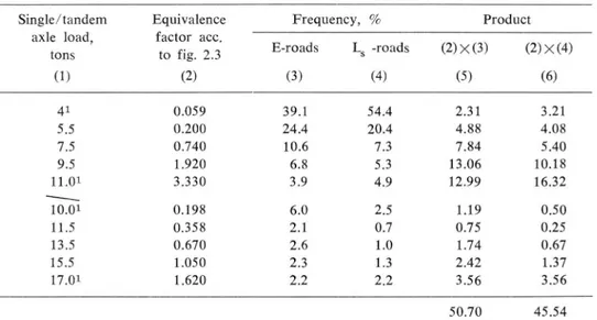
The numerical “group midpoint” and the equivalence factors corresponding to them have been listed in table 2.4, columns 1 and 2 respectively. The table also states the frequencies within each group for two of the road categories (E and L s ), which represent the highest and the lowest road standard. These frequencies are given in columns 3 and 4.

Table 2.4. Data required for calculation of an average equivalence factor for each axle application. Single/tandem axle load, tons (1) Equivalence factor acc. to fig. 2.3 (2) Frequency, % Product E-roads (3) Ls -roads (4) (2) X (3) (5) (2) X (4) (6) 41 0.059 39.1 54.4 2.31 3.21 5.5 0.200 24.4 20.4 4.88 4.08 7.5 0.740 10.6 7.3 7.84 5.40 9.5 1.920 6.8 5.3 13.06 10.18 11.01 3.330 3.9 4.9 12.99 16.32 T o o i 0.198 6.0 2.5 1.19 0.50 11.5 0.358 2.1 0.7 0.75 0.25 13.5 0.670 2.6 1.0 1.74 0.67 15.5 1.050 2.3 1.3 2.42 1.37 17.01 1.620 2.2 2.2 3.56 3.56 50.70 45.54

If the frequencies in columns 3 and 4 are weighed together with the equivalence factors in column 2, and the products 5, 6 summed, the result will be a weighted, average equivalence factor for every axle application on roads of category E and L s respectively. The sums in columns 5 and 6 refer to an axle load of 8 tons. Since the Swedish design regulations are based on an axle load of 10 tons, these sums should be converted to a 10-ton axle load. This conversion, too, can be made with the aid of the diagram in fig. 2.3.

(26)

The results from table 2.4 will be:

Roads of category E: 0.44 X 0.507 = 0.22

Roads of category L s : 0.44 X 0.455 = 0.20

This result means that every axle application corresponds on the average to a load equivalent to 20— 22 % x of that from a 10-ton axle. The traffic load in respect of the axle load of the individual vehicles is thus practically the same for roads of categories E and L s .

The curves in fig. 2.4 are based on 1,216,516 axle applications. The cor

responding number of vehicles was 438,110. On the average, then, each vehicle can be regarded as corresponding to 2.8 axles. Each vehicle passage thus exerts a load which on the average is equal to approx. 0.7 10-ton axles. With a traffic volume of between 250 and 1,000 freight vehicles/24 hours (column 4 in table 2.3), the corresponding load will be 175— 700 (averaging 435) 10-ton axle applica tions/24 hours, which is equivalent to 64,000— 255,000 (averaging 160,000) 10-ton axle applications/year.

It was established earlier that the pavement thicknesses given for the 9-metre and 13-metre sections can withstand a load of approx. one million axle applica tions of a 10-ton axle load. If this total load is compared with the annual load calculated above on the assumption that both lanes of a two-lane highway are subjected to equal loads, the service life of the pavement would be between 31 and 8 years, or on the average about 13 years. At the end of this period, the service ability of the pavement will have been reduced to a PSI-value of 2.5, which accord ing to the AASHO Road Test means that extensive repair work will be necessary in order to restore the pavement to a condition acceptable to traffic.

The calculation thus shows that a pavement designed according to design column 4 (table 2.3) will need to be repaired after about 13 years, for instance by resurfacing. In extreme cases (an average of 1,000 freight vehicles/24 hours), this need may arise after only 8 years. These time intervals are in rather good accordance with those found by practical experience.

The calculation above is based on the assumption that the effect of an axle application is not influenced by the season during which it occurs. There is, how ever, nothing to prevent the modification of this assumption — which, indeed, was done in the AASHO Road Test — by introducing a seasonal weighting function, by which the number of axle applications is to be multiplied. By this means, a greater weight (more than 1) could be accorded to applications during the thawing period than to those occurring during the other seasons, and this would lead to a higher average equivalence factor than that calculated above. On the other hand, 1 With the estimated values 12/18 instead of 11/17 tons the result will be 23— 25 instead of 20—22 %.

(27)

the applications during the frozen period would be weighted with a multiplier of lower weight — perhaps equal to or close to 0 — and this would have the opposite effect. As this latter period is longer than the sensitive thawing period, the calcula tion made above may be considered to be sufficiently accurate and to result in an equivalence factor which at any rate is not too low.

There is, however, no reason to introduce into this rough calculation any sea sonal correction, as the assumptions in other respects are uncertain. The results of the calculation are therefore to be interpreted merely as guide values.

On the basis of the rough calculations described it may be assumed that the costs specified in table 2.1 can be regarded as corresponding to about one million applications with an axle load of 10 tons. One may now ask how the costs would

have changed if the axle load had instead been 8, 12 and 14 tons.

This problem will be studied in the following sections.

2.4 Costs for Axle Loads of 8? 12 and 14 tons

Before those differences in costs can be determined which are brought about by axle loads of 8, 12 and 14 tons as opposed to 10 tons, it will first be necessary to calculate the corresponding pavement thicknesses.

This will be done below, partly on the basis of the theory of elasticity and partly on the basis of the results from the AASHO Road Test.

2.4.1 Calculation Based on the Theory of Elasticity

The design chart drawn up at the Swedish Road Research Institute, which is based on the theory of elasticity (9), can be used to determine the difference in pavement thickness necessitated by a change in the permissible axle load. This difference has been found by calculation to amount to approximately 12 % (4) for an in crease in the axle load from 8 to 10 tons for a bed soil equivalent to that of material group C.

The same result is reached in a publication issued by the International Road Transport Union (10), where the necessary pavement thickness for both 10-ton and 13-ton axle load has been calculated from a diagram drawn up by Ivanov (11), whose calculations are also based on the theory of elasticity. It is then assumed that the deflection under a wheel is less than 0.15 cm.

This calculation shows that a 3-ton increase in the axle load necessitates an in crease of 18 % in the pavement thickness. This may be considered to correspond to 12 % for an increase in the axle load from 8 to 10 tons.

(28)

According to these calculations, based on the theory of elasticity, it appears that if the axle load is increased from 8 to 10 tons, the pavement thickness will in crease by about 12 %. It should be borne in mind, however, that the number of axle applications is assumed to be the same after the introduction of an increased axle load as before. This will mean that the tonnage of freight which can be carried on the highway after the axle load has been increased will be greater than before. A comparison on these grounds will therefore not present a fair picture from the standpoint of transport economy.

A more correct comparison must instead assume that the total tonnage of freight moved will remain constant irrespectively of the magnitude of the permissible axle load. This means that allowance is made for the decrease in the number of axle applications made possible by an increased axle load without any change in the total tonnage moved. The results reported from the AASHO Road Test are, in fact, based on systematically giving due consideration to both axle load and axle applications. It may therefore be of interest in this context to study how much the number of axle applications influences the difference in pavement thickness, cal culated on the basis of the theory of elasticity.

2.4.2 Calculation Based on the Results of the AASHO Road Test

The ideal pavement thickness is that which can be adapted exactly to the traffic load — axle load and number of axle applications — to which the highway struc ture will be exposed during its anticipated service life. In practice, however, such exact adaptation cannot possibly be attained. As a rule, most roads are either underdimensioned or overdimensioned, and consequently do not provide the eco nomically soundest solution.

If the increase in pavement thickness and pavement construction cost caused by a certain, specific increase in the axle load is to be determined, it must be assumed from the start that the pavement is designed in accordance with a theoretical traffic load and that the tonnage carried on the road is constant.

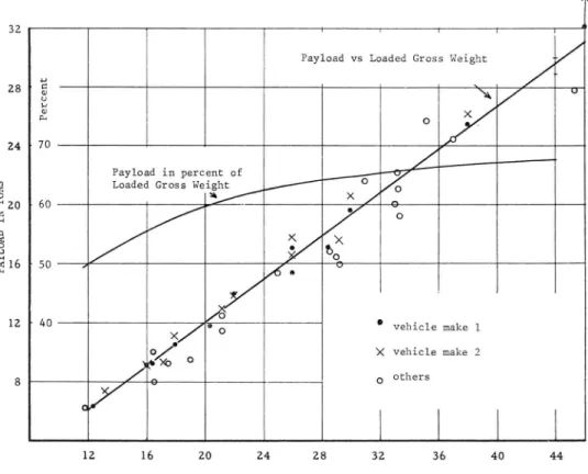
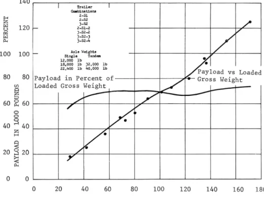
According to a publication issued by the Swedish Road Research Institute (12), the following relationships between axle load and vehicle payload are valid for a 2-axle truck:

Axle load, tons Payload carried,

Front Rear tons

5 8 6.8

6 10 9.0

6 12 10.4

(29)

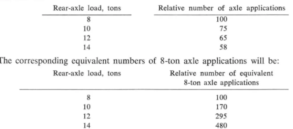
If it is assumed that the said truck can utilize different rear-axle loads (8, 10, 12 and 14 tons), the number of axle applications necessary to move the same tonnage will thus be:

The corresponding equivalent numbers of 8-ton axle applications will be:

On the basis of the number of equivalent 8-ton axle applications it is possible to determine graphically an approximate value of the thickness index, D, from the diagram mentioned in the reports from the AASHO Road Test (13). This diagram

is reproduced in fig. 2.5. L o o p s

N o.

10 MILL.

Fig. 2.5. Relationship between pavement thickness and number of axle applications according to the AASHO Road Test at PSI = 2.5.

Rear-axle load, tons Relative number of axle applications

8 100

10 75

12 65

14 58

Rear-axle load, tons Relative number of equivalent 8-ton axle applications

8 100

10 170

12 295

(30)

When, as in this case, differences are to be calculated, it is appropriate, especially for 7V-values (N = number of axle applications) which are very close to one another, to form an analytical expression for the 8.2-ton curve in fig. 2.5, i.e. to express a functional relationship between thickness index D and the number of axle applications N.

This functional relationship can be expressed by the following formula:

Z) = 0.689 • N 0135-0 .5 ... 2.1. This equation describes with good accuracy the relationship between D and N which is illustrated by the 8.2-ton curve in fig. 2.5.

Using this equation, values of D can be calculated for the number of equivalent 8-ton axle applications corresponding to axle loads of 8, 10, 12 and 14 tons, thereby making it possible to calculate the differences in pavement thickness necessitated by a 2-ton increase in the axle load.

If it is assumed that the number of axle applications in the case of an 8-ton axle load is 1 million, the results will be those given in the following table.

Axle load, tons N o. of equivalent 8-ton axle applications Thickness index, D Difference in D % 8 10 1.00 x i o 6 1.7 0 X 1 0 6 3.95 4.28 8.4 7.9 7.6 12 2.95 X 106 4.62 14 4.80X 106 4.97

The results from the AASHO Road Test can be applied directly only if the con ditions are the same as in that test, including also the nature of the road bed material, which in the AASHO Road Test was equivalent to a CBR-value of 3. As explained earlier, the average bed material referable to table 2.1 can be con sidered equivalent to a CBR-value of 10. For this reason, it is here of importance to take a CBR-value of 10 instead of 3 as the starting point when calculating the difference in pavement thickness necessitated by an increase in the axle load.

A calculation of this kind can be made with the aid of the nomograph in fig. 2.2, which has been drawn up on the basis of a PSI-value of 2.5. At this serviceability level (PSI = 2.5), the quality of the surface has, according to the AASHO reports, reached the limit at which extensive improvement measures are considered to be necessary even if the road may still be regarded as usable. When the PSI is lower than this, for instance 1.5, the road surface is considered to be in such poor con dition that reasonable demands on driving comfort and safety can no longer be satisfied. It therefore seems reasonable to choose the figure 2.5 as the lower PSI- limit.

(31)

The following figures are found by using the nomograph:

This calculation gives roughly the same difference in the value of Dt as the dif ference in the value of D derived earlier from the equation 2.1. The relative difference, in contrast, will be greater when CBR = 1 0 than for CBR = 3.

Corresponding calculations based on other figures for the number of axle applications in the case of an 8-ton axle load than that applied here (1 million) can be carried out in a similar way as in this example.

The calculations according to equation 2.1 have been included here merely for the purpose of comparison, since as stated earlier they are not applicable to a CBR-value of 10.

On the basis of the calculations outlined above it may be assumed that an in crease of 2 tons in the permissible axle load with an unchanged total tonnage of freight moved necessitates an increase in the pavement thickness (properly the thickness index) by (in round figures) 11, 9 and 8 % respectively for the three axle-load intervals.

As stated earlier on, calculations based on the theory of elasticity lead to a higher increase. The difference in results is primarily due to the fact that calculations based on the theory of elasticity do not make allowance for the reduction in the number of vehicle trips made possible by an increase in the axle load if the tonnage of goods moved is assumed to remain constant.

The difference may be due secondarily to the different assumptions on which the methods of calculation are based: on the one hand results presuming com pletely elastic conditions in the pavement and road bed materials, on the other hand empirically derived results from field tests.

Since it must be considered correct from a technical and economic standpoint to assume that the tonnage moved will be the same after an increase in axle load as before, the second of the two methods presented should give the best estimate of the necessary increase in pavement thickness. This increase can therefore be assumed to correspond to the percentages stated above. As can be seen, however, the difference between the two methods is only small.

It is now necessary to investigate the increase in cost that results from an in crease in pavement thickness. Naturally, this depends on the material used and the thickness chosen for each of the three pavement courses. We illustrate this in the

Axle load, tons N o. of equivalent 8-ton axle applications Structural number, » t Difference in D t % 8 10 1.00X 106 1.70X 106 3.25 3.60 10.8 8.4 7.7 12 2.95 X 1 0 6 3.90 14 4.80 X 106 4.20

(32)

following manner by investigating a surface course and the base and subbase course beneath it.

In the analysis of pavement costs in section 2.1 above, the following price rela tionship was found between the various courses which together form the pavement:

A “normal” pavement may have the following structure:

This pavement is equivalent to a thickness index, D, of 3.9 in. or 9.8 cm. As shown by the formula

D = 0.44-D 1 + 0.13- D2 + 0.11 D 3

the quantities D u D2 and D3 can be combined in infinitely many different ways for the same value of D. The validity of the formula assumes only that D x is not less than 5 cm and that D2 is not less than 7.5 cm. An increase of D by, say, 9 % , can therefore lead to different cost increases, depending on how the requisite increase in thickness is shared out among D l9 D2 and Ds.

The extreme values will be:

The biggest cost increase occurs if only D 1 is increased. The smallest cost increase occurs if only Ds is increased.

Application of the price relationship above yields the following results.

If only £>! is increased by 9 % (0.9 cm), the value of the first term in the equa

tion will be 3.1 instead of 2.2 cm. The increase in will then be 2.1 cm, which

means that D x is increased from 5 to 7.1 cm. Therefore, the ratio between costs after and before the thickness increase will be:

7.1X 15.5 + 20X 2.3 + 45

--- = 1.19, 5X 15.5 + 20X 2.3 + 45

which shows that the incremental cost will be 19 %.

If only Ds is increased, an increase of = 8 .2 cm will be necessary.

Material Cost, kronor/sq.metre Price relationship

per cm

Bituminous surface 1.70 15.5

Base course 0.25 2.3

Subbase course 0.11 1

Material Thickness of course, cm Price, kronor/sq.metre

Bituminous surface 5 8.50

Base course 20 5.00

Subbase course 45 4.95

(33)

By analogy, we get:

5X 15.5 + 20X 2.3 + 53.2

--- = 1.05, 5X 15.5 + 2 0 X 2 .3 + 4 5

and the incremental cost in this case will thus be 5 %.

The biggest cost increase will be 19 % and the smallest 5 %.

As can be seen in table 2.3, this latter alternative is not in keeping with the principles in the Swedish design standards, while the former for financial reasons is not applicable in practice. Both of these extreme alternatives can thus be excluded.

What remains, then, is a distribution of the thickness increase in a suitable manner between all the courses. This distribution can for instance be such that we obtain a linear relationship between thickness index and costs. An increase in thickness index by 9 % thus corresponds to a cost increase of 9 %. We find that this can be obtained by, e.g., increasing the thickness of the bituminous surface by 0.45 cm (10 kg/sq.m), that of the base course by 1.8 cm and that of the subbase by 4 cm. Such a distribution is likely to be regarded as suitable by most highway engineers. In the following we can therefore assume that the percentages calculated above for the increase in thickness index are valid for the corresponding increase in pavement cost.

However, in the road section studied above the side slopes are not included. Obviously, the increase in the quantity of base and subbase material will be slightly higher than the increase in pavement thickness. For the road widths and axle loads studied here it can be shown that this increase in quantity will be 1.5— 2.5 % higher than the increase in pavement thickness. This is allowed for in the following by adding an average of 2 % to the percentages calculated above. The inaccuracy involved by choosing a constant value for this allowance is only minor.

2.4.3 Costs of increased Roadbed Width, Drainage and Right of Way

A thicker pavement necessitated by a higher axle load requires a larger width of the roadbed than a thinner one. Therefore increasing costs due to additional earthwork (cuts and fills), drainage and right of way would also be related to rise in axle loads.

A calculation prepared by the Road Administration shows that the amount of the cost increase for additional cuts and fills is less than 1 % of the total cost for the pavement, when the axle load increases from 10 to 13 tons.

The additional costs due to extra drainage and right of way are difficult to cal culate generally but can be estimated to be of the same magnitude as mentioned above.

(34)

In this study, an additional allowance for increased roadbed width, extra drainage and right of way is estimated to an average of 2 % of the pavement construction costs for every 2-ton increase in axle load.

The increase in pavement construction cost including this allowance will be as follows.

2.4.4 Bridge Construction Costs

The costs discussed so far relate to highways only. However, if the permissible axle load on a highway network is increased, it must also be increased for the bridges included in that network. As the construction cost of a bridge exceeds that of a road of the same length, it is necessary to study the extent to which the bridge construction cost influences the average incremental pavement cost. According to information provided by the Road Administration (14), it may be assumed that an increase in the design tandem-axle load from 20 to 24 tons, (and higher gross weights) should result in an increase of approx. 7 % in the bridge construction cost. For an assumed bridge width of 13 metres and an average cost per sq. metre of

1,000 kronor, the construction cost will be about 15 times greater than for a high way of the same width.

Since, as in this case, the average cost per kilometre of the highway network is to be determined, the cost per kilometre should, strictly speaking, be calculated as a weighted average between the road (pavement) part and the bridge part. Swedish bridges in 1965 were estimated to cover a length of 265 kilometres (9,200 bridges with an average length of 28.5 metres). If this is considered in relation to the total length of the Swedish road network, approx. 97,000 kilometres, it is found that on the average there is 1 bridge per 10 kilometres of road, or approx. 3 metres of bridge per kilometre of road.

Obviously, it is a complicated matter to determine the increase in bridge con struction cost generally since the cost-increase depends on bridge type, bridge span, type of foundation structure, etc. As in some types of bridges, an increased axle load affects a greater part of the bridge structure than in others precise calculations can only be made in specific cases.

The already mentioned increase of 7 % has been determined as an average for different bridge types. As no other cost data are available this figure will be used here as corresponding to the increase in tandem-axle loads ranging from 20 to 24 tons.

Increase in axle loads from— to

Increase in pavement construction cost in per cent

8— 10 15

10— 12 13

(35)

For the other two axle-load intervals no calculations have been made and therefore rough estimates are necessary.

We assume that the increases between 16 and 20 and between 12 and 16 tons amount to 8 and 9 % respectively. The average cost, 1,000 kronor per sq. metre, stated earlier is assumed to be related to a tandem-axle load of 20 tons, and the service life corresponding to this original cost is estimated to be 50 years, i.e. approx. twice the service life of the pavement.

This difference in estimated service life is compensated for in table 2.6, where the construction cost of the average bridge part per kilometre of the road network is added to the construction cost of the pavement part.

2.4.5 Maintenance Costs

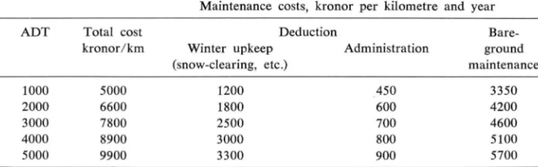
The Road Administration has compiled data showing the actual maintenance costs for three different highway sections with different traffic intensities.

The results for roads with a bituminous surface are presented in table 2.5 below. Table 2.5. Annual maintenance costs for a 13-metre wide road in southern Sweden in

relation to ADT.

Maintenance costs, kronor per kilometre and year

A D T Total cost Deduction

Bare-kronor/km Winter upkeep Administration ground

(snow-clearing, etc.) maintenance

1000 5000 1200 450 3350

2000 6600 1800 600 4200

3000 7800 2500 700 4600

4000 8900 3000 800 5100

5000 9900 3300 900 5700

Using these figures (table 2.5) as a guide, the following maintenance costs can be estimated for the 3 sections for which the costs have been calculated:

The maintenance costs listed in table 2.5 are not referable to any specific axle load but correspond instead to the axle loads which are normally encountered. When, as in this case, we are concerned with calculating the difference in pavement construction costs arising out of different axle loads, a question which arises is if maintenance costs also increase with increasing axle load. If so, the discounted

Highway section, Maintenance cost, kronor per km

m and year

13 6000

9 4000